In the preceding recipe, we saw a quick option for formatting across the entire workbook, which was great. However, there can be situations where we need some specific formatting within a particular worksheet. Let us see the following recipe to see how we can do formatting within a particular worksheet.
We will continue working in our existing My first Tableau Workbook workbook and use the already connected CoffeeChain Query (Sample - Coffee Chain) data source. Let us see how this is done.
- Let us create a new sheet and rename it as Formatting within a Worksheet.
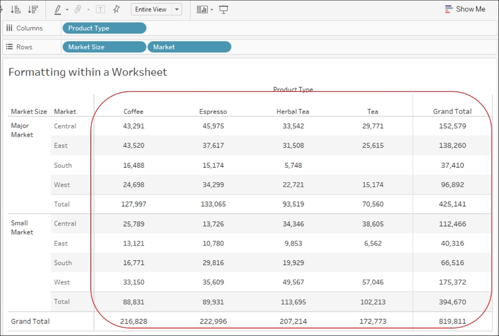
- Next, let us make sure that we select the CoffeeChain Query (Sample - Coffee Chain) data source from the Data pane. Following this, we will create a text table by dragging the Product Type field from the Dimensions pane and dropping it into the Columns shelf, followed by dragging the Market Size field from the Dimensions pane and dropping it into the Rows shelf. Next, we will drag the Market field from the Dimensions pane and drop it into the Rows shelf, just next to the Market Size field. Lastly, let's drag the Sales field from the Measures pane and drop it into the Text shelf. This will create a view as shown in the following screenshot:

- Once we are done creating our basic view, let us then add our Totals and Subtotals by dragging the Totals option from the Analytics pane and selecting the Subtotals, the Column Grand Totals, and also the Row Grans Totals. Refer to the following screenshot:

- Once we enable our totals, our view will update, as shown in the following screenshot:

- As we can see, our worksheet currently has a lot of white space around a text table. To change this, let's click on the dropdown in the toolbar that currently reads as Standard and let's change it to Entire View. Refer to the following screenshot:

- This action will update our view to what is shown in the following screenshot:

- Next, let's click on the Format option in the toolbar and select the Font… option. This will show a new section on the left-hand side that reads as Format Font. Refer to the following screenshot:

- The current workbook font type is Tableau Regular with a font size of
9pt. Even the Total and Grand Total have the same font type and font size. Let's quickly change the font size of Grand Total from9ptto10ptin the Pane: section as well as the Header: section. Refer to the following screenshot:
- This will change the font size for both the Grand Total text and the Grand Total numbers. Refer to the following screenshot:

- As a next step, let us change the alignment for the Sales number from right aligned to center aligned. To do so, let us click on the Alignment icon, which is next to the Font icon. Refer to the following screenshot:

- Under the Default | Pane section, let us change the alignment from Automatic to Center. Refer to the following screenshot:

- This will update our view, as shown in the following screenshot:
- As a next step to formatting, let us remove the gray bands and color only the Grand Total sections. To do so, let us click on the Shading icon on top, which is next to the Alignment icon. Refer to the following screenshot:

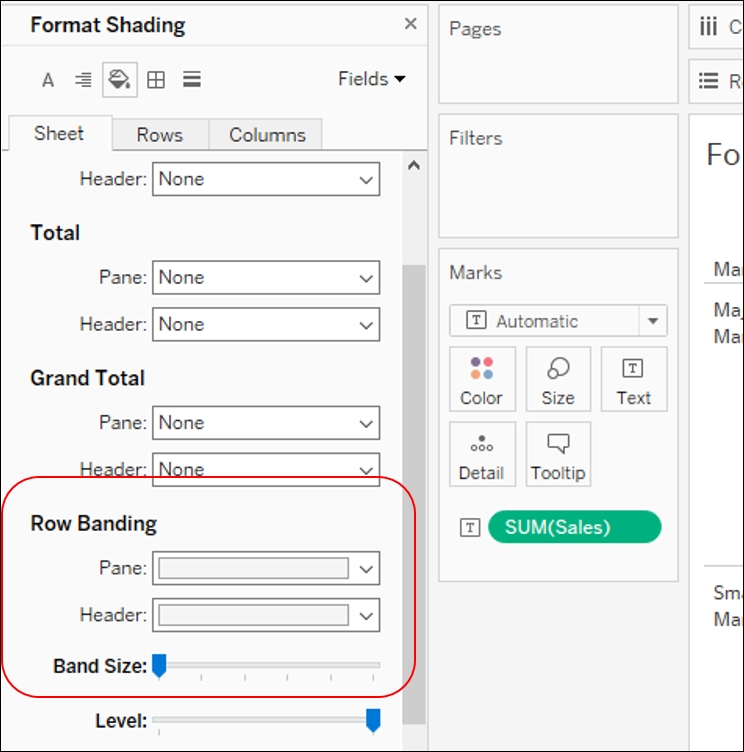
- Once we are in the Format Shading section, we will go to the Grand Total section and click on the dropdown for Pane; to select a gray color. Refer to the following screenshot:

- After we are done with that, we will go to the Row Banding section and move the Band Size: slider to the left most side or lower side. Refer to the following screenshot:
- Both these actions will update our view, as shown in the following screenshot:

- Now let's also add some of the column dividers between different product types. To do so, let us click on the Borders icon, which is next to the Shading icon. Refer to the following screenshot:

- Let's scroll down to the Column Divider section and move the Level: slider to the right most side or higher side. Refer to the following screenshot:

- This action will update our view, as shown in the following screenshot:

- Notice the sales values, currently there is no way for our end users to find out what currency they are looking at. We know that these are US dollar values, so let us go ahead and change the number format of our sales values. To do so, let us click on the dropdown that says Fields and select the SUM(Sales) option. Refer to the following screenshot:

- This will update our Format section, as shown in the following screenshot:

- Let us select the Currency (Standard) option from the first Numbers: section and then select the English (United States) option. Refer to the following screenshot:

- This will update our view, as shown in the following screenshot:

- Lastly, let us remove the word Product Type from the top of our view and to do so, we will right-click on the Product Type text and select Hide Field Labels for Columns. Refer to the following screenshot:

- This will update our view, as shown in the following screenshot:

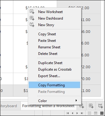
The preceding recipe explains how we can format the objects within our worksheet. In case we need the similar formatting across multiple worksheets, then instead of formatting the relevant sheets individually, we can simply format one sheet and copy and paste the formatting to the other sheets.
To do so, all we need to do is right click on the sheet tab and select the Copy Formatting option and then go to the relevant sheet and select the Paste Formatting option. Refer to the following screenshot: