4

Interactive Time-Based Art

In this project, you’ll explore time as a variable and put it to use as a driving force in some time-based art—that is, art that develops over time. At first, this concept may seem a bit abstract. It’s meant to! Your final sketch will be a clock, and its appearance will be based on what the code you write does over time.

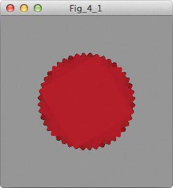
By now, you’ve learned and used many of the basic structures and functions in Processing. Think of this as a chance to just play with and explore variables within your current knowledge and understanding. For example, with what you know now plus what you’ll learn in this project, you’ll be able to draw shapes at different angles, to impressive effect. I created the sawblade pattern in Figure 4-1 by rotating a rectangle every second and using a time-based variable to change the color from black to red.

FIGURE 4-1: This simple time-based artwork rotates and changes color based on the second hand of a clock.

Since your creation will be constantly changing, I’ll forgo the paper and pencil this time and jump right into the code. Go ahead and get lost for a bit, but never lose track of time as a variable!

BUILT-IN VALUES

To change a shape’s dimensions, color, or other properties while your sketch is running, you need to be able to change the values you pass to your Processing functions without adjusting the sketch and restarting. You created variables to automate such changes in Project 3, but say you want a shape to respond to the passage of time or even to a mouse click.

In that case, you also have at your disposal a powerful set of system variables that are built into Processing, as well as several useful system functions. Both let you harness values from your computer to use in your projects, and you can use them in any part of your Processing sketch. Your system functions return values from your computer, such as the date, time, and so on, and for all intents and purposes, you can treat them the same as system variables.

You’ll explore system variables and functions in this project as you create dynamic and time-based art. Let’s take a quick look at a few particularly useful system variables now.

Finding the Mouse and Keypresses

You’ve already played around with two of the system variables I’ll describe. Remember mouseX and mouseY? Those are mouse, or cursor, system variables. Here are the mouse system variables and the values they contain.

mouseXThe x-coordinate of the mouse cursor while it is in your sketch window

mouseYThe y-coordinate of the mouse cursor while it is in your sketch window

pmouseXThe x-coordinate of the mouse cursor from the previous frame

pmouseYThe y-coordinate of the mouse cursor from the previous frame

keyThe ASCII numerical value of a letter or number being pressed

The mouseX and mouseY variables store your mouse’s current position, while pmouseX and pmouseY store its previous position. The key variable stores any letter or number key you’re currently pressing!

Telling Time

Your computer has a built-in clock, and Processing can access it and store certain time-related values for you to use with certain functions. You can access all sorts of time- and date-based information for your sketches. Here are a few time-related functions that you’ll find useful.

millis()The number of milliseconds since the sketch started

second()The seconds value on your computer’s clock

minute()The minute value on your computer’s clock

hour()The hour value on your computer’s clock

day()The day value of the date on your computer’s calendar

month()The numeric value of the current month on your computer’s calendar

year()The year from your computer’s calendar

All of these functions return a time-related number. Use them to represent the passing of time—from the number of milliseconds since you clicked Run to the current calendar year—in your sketch!

Putting Built-in Values into Action

You can use the values I’ve described in this section anywhere you would normally pass a number. For example, you can use second() to change a rectangle’s shade of red based on how many seconds have passed in the current minute:

Just pass second() as the red value of the rectangle’s fill() function!

If you run that code as a sketch, it probably isn’t the most exciting thing to watch. It takes 60 seconds to get to a measly 59 out of 255 for our red value. But you can up the ante a bit and give a possible range of 0 to almost 255. Enter math!

EXTENDING YOUR RANGE

In the color example in the previous section, the red value will only go up to 59 because I used the value returned by second(). If you want a wider range of values, you can multiply the second() variable by, say, 4. When you choose a multiplier for any value you want to pass into a function, think about the range of values the function will actually accept. The fill() function accepts only a number between 0 and 255 for any color value. Your computer won’t explode if you go over; it just caps out at 255.

The highest value you’ll get from second() is 59, so when you multiply that by 4, the highest value you’ll pass to fill() is 236, which is still within the fill() function’s limits. Try this as a comparison to the previous example:

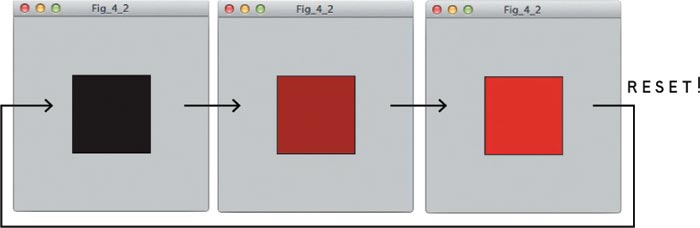
As shown in Figure 4-2, the red value of the rectangle changes every second. When you start the sketch, the value passed from second() is 0, and the rectangle is black; as the second() value increases, so does the red value in the fill() function, and the rectangle becomes redder. After the second() value hits 59 and the red value peaks at 236, the second() function starts over again at 0—a black rectangle.

FIGURE 4-2: This rectangle’s shade of red changes according to the value of the second() function, as if second() were a variable.

Notice that the syntax of the fill() function didn’t change, even though you’re using an equation within the parameter for the red value. If you moved or removed the comma, you would get an error when you tried to run the sketch.

The value of second() is small and changes slowly, so I multiplied it to increase the rectangle’s range of redness and speed up the color shift. A similar concept applies to values that change quickly or grow large, like those obtained from millis() or mouseX. Just subtract or divide to get a smaller or steadier value! If you want a value in your sketch to be based on time or some other variable, but the variable changes at a speed you don’t like, amplify or reduce it using mathematical operators.

TRANSFORMATION FUNCTIONS

When you manipulate a shape’s dimensions, coordinates, and so on, you’re transforming the shape. Geometric transforms include scaling, rotating, and translating, and you may see some similarities between transforms of the same name in graphic design software and what you learn in this project. Here are a few transformations that you’ll use in this book:

scale(S)Scales the entire sketch by a percentage (S) in decimal form (for example, 80% = .80)

rotate(R)Rotates the sketch by R radians (3.14 radians = 180 degrees)

translate(X,Y)Moves the sketch X pixels along the x-axis and Y pixels along the y-axis

For now, use the transformation functions sparingly, as they’ll be applied to everything in your sketch. For example, look at the translate() function in action.

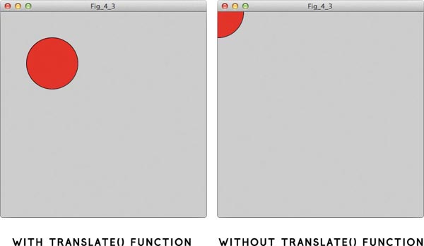
Normally, you’d expect ellipse(0,0,100,100) to draw an ellipse at the origin of the sketch window. But because translate(100,100) is called before the ellipse() function is called, the ellipse will be shifted by 100 pixels on both axes, as shown in Figure 4-3.

Later, I’ll show you how to apply a transformation to a specific shape or group of shapes, but for now, time to dive in and make a clock!

FIGURE 4-3: An ellipse translated to the right by 100 pixels and down 100 pixels

AN ABSTRACT CLOCK

Up to this point, I’ve just talked about time-based values, but now you’ll get your hands dirty and actually use those values in code. Any time you learn a new Processing concept, I recommend running parts of the code in small sketches that look like the example code from this book. When you’re practicing, the goal is to quickly understand the function or concept, rather than create something elaborate and beautiful.

Comparing the Major Time Functions

First, I’ll compare four of the major functions that return time values. The following example uses second(), minute(), hour(), and day() to create an abstract clock, where rectangles move according to the time on your computer’s clock. I replaced some fill() function and shape parameters with these built-in values. Since time-based functions change over time, you will have to rewrite the code on your own machine, as shown in Listing 4-1.

LISTING 4-1: An abstract clock with three moving rectangles

This chunk of code uses the second, minute, and hour hands of the clock on your computer. Since there are 60 seconds in a minute and 60 minutes in an hour, I set the width of the sketch window to 240, which is 60 multiplied by 4.

For the first rectangle, I multiplied second() by 4 to give both its red value ❶ and x-coordinate ❷ a minimum of 0 and maximum of 240. The second and third rectangles follow that pattern, using minute() and hour(), respectively. I replaced the x-coordinate with a time-based value in both cases, but in one, the minute() value controls the green fill() argument, and in the other, the hour() value controls the blue fill() argument.

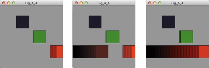
You can see the results in Figure 4-4. If you want to expand on this sketch, add a fourth rectangle that uses millis(). I will leave it up to you to figure out the equation to have the rectangle track across the screen properly and change color.

FIGURE 4-4: An abstract clock using Processing. The top rectangles represent hours, the middle rectangles represent minutes, and the bottom rectangles represent seconds.

These values are really useful for triggering events at specific times, having shapes move on their own (as demonstrated here), or changing color over time. Now you can put all this into practice and make your clock more stylish.

Spicing It Up!

In this section, I’ll show you how to create another abstract clock that is a little more intricate than the previous one. The clock isn’t really useful for getting to work or school on time, but since I designed the project I’ve become accustomed to looking at it, and I’m actually pretty good at telling what time it shows. Practice reading your clock, and you can impress your friends by being able to tell time from a group of shapes that move and change color!

First, think about what you want your clock to do. You know that you want it to react to time, so you’ll be using the millis(), second(), minute(), and hour() functions.

I started with the example code from Listing 4-1 and changed it for this project. The original abstract clock sketch has good potential, but I wanted to make the clock a little more creative. I also wanted to include either scale() or rotate() in the sketch.

Start by creating a setup() and draw() loop. Then add some shapes that move and leave trails as they change color and move across the screen. Let’s also include shapes that stand alone, without trails; you’ll be able to tell that these shapes move only if you actually watch them over time.

Listing 4-2 shows the complete code for the project.

LISTING 4-2: A more intricate abstract clock

First I played with the size of the seconds-based rectangle and tried rotating the sketch as well. I also commented out the background() function ❶ from the draw() loop so my sketch would leave a trail of shapes.

This modified abstract clock uses three different shapes: our original rectangle ❸, a triangle ❹, and an ellipse ❺.

The biggest difference in the sketch itself is probably that the shapes are rotating around the sketch origin (0,0). I created this effect using the rotate() function at the top of the draw() loop ❷. The rotate() function accepts a single parameter, and I’ve used millis(). I wanted something that changed relatively quickly, and the number of milliseconds since the sketch started fit the bill nicely. Since the value of millis() is not connected directly to your system clock, but rather internally within your sketch, it also gives you a good source of time that is independent from your system clock for future applications.

The if() statement at the end of the draw() loop redraws the background to clear the shape trails any time seconds() is greater than or equal to 59 ❻, which would be roughly the end of a minute. Run the code and watch it for a bit. At the end of each minute, you should see everything disappear as the background is redrawn, and the clock should start over again.

Of course, you could redraw the background whenever you want. For example, try changing the number in the statement from 59 to 10. This would redraw the background when the second hand was at 10 seconds and higher. How long do the shape trails stay visible?

As you move through the code it should look pretty familiar compared to the earlier example sketch. Feel free to change things and make this your own! Play around with using a combination of your mouse variables and your time variables to change color, shape, or position within your code.

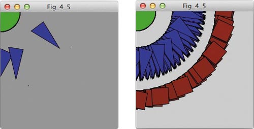
I ran this piece of code around noon and saw the colors shown in Figure 4-5. It would be interesting to see this sketch at the time you run it! The colors your sketch will produce while you’re reading this book will probably be different from mine.

FIGURE 4-5: The new abstract clock, starring three different shapes

SHARING YOUR PROJECT!

Now that you’ve tried my version of this project, make it your own, make it beautiful, and make it a piece of art. When you’re done, you could even share it on OpenProcessing.org, so everyone can benefit from your work and creativity.

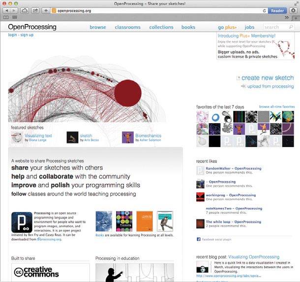
First go to http://openprocession.org/ and follow the instructions there to register an account. Once you have an account, you’ll land on your dashboard, which should look similar to Figure 4-6.

FIGURE 4-6: OpenProcessing dashboard

From your dashboard, you can access sketches you’ve recently uploaded or created using OpenProcessing’s web-based IDE. You can click create new sketch to try out the IDE, but for this book you should stick to the original Processing IDE for consistency and functionality.

You can also upload sketches you created with the normal IDE, so try it with your abstract clock project (Listing 4-2). Click upload from processing to reach the screen in Figure 4-7, which gives basic instructions and, perhaps more importantly, the limitations on what you can upload to OpenProcessing. You can’t upload anything over 10MB, but the abstract clock file is well below that limit.

FIGURE 4-7: Upload instructions from OpenProcessing

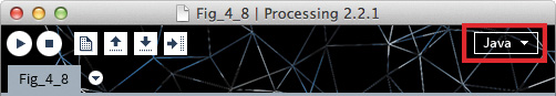
Save your sketch if you haven’t already done so. You now need to install JavaScript mode for Processing, which is a short and painless process. Click the Mode drop-down menu (highlighted in Figure 4-8); you should see only Java and an Add Mode option. Select Add Mode to bring up the Mode Manager window. From here you can select which modes to add to Processing. At the time of writing, there are a number of available modes, which you will explore later in the book. For now, find JavaScript mode and click Install. The installation will take a few minutes, and then you are done!

FIGURE 4-8: The Mode drop-down menu is currently set to Java.

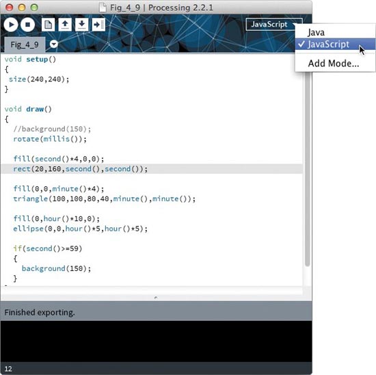
Click the Mode drop-down menu again, and you should now see two mode choices: Java and JavaScript. Select JavaScript. Your sketch should disappear and reappear quickly with a different-looking control bar at the top of your sketch, shown in Figure 4-9. The Mode drop-down menu now says JavaScript. Congratulations! You’re ready to send your code to the Web.

FIGURE 4-9: The Processing control bar changes for JavaScript mode.

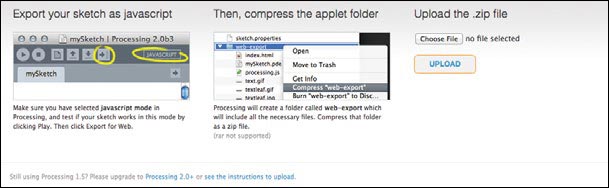
Learning JavaScript would require a book of its own, so for now, all you need to know is that Processing’s JavaScript mode allows you to create JavaScript programs using the Processing language and export your sketches to a web-friendly format. Just click the Export for Web button; it’s the last button in your toolbar and looks like an arrow pointing to the right, as shown in Figure 4-10. This creates a folder called web-export inside your sketch folder. This new folder should contain three files: a copy of your sketch, the processing.js file, and index.html, which is the web page of your sketch.

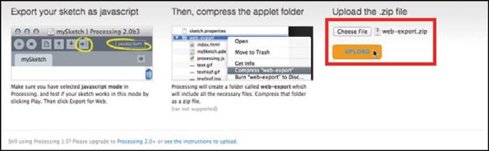
Now, compress or zip the web-export folder so you can upload it to OpenProcessing. In Windows, right-click the folder and select Send to Compressed (zipped) folder. Then return to OpenProcessing, click Choose File, navigate to your sketch folder, and select the zipped web-export folder. Click Upload, shown in Figure 4-11, to send your sketch to OpenProcessing.

FIGURE 4-10: Exporting your sketch for the Web

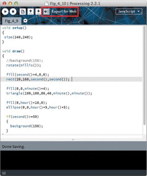
FIGURE 4-11: Uploading the web-export folder to OpenProcessing

OpenProcessing should take you to a new page to add a name, thumbnail, and description to your sketch. The website will also show your sketch below this interface, as in Figure 4-12.

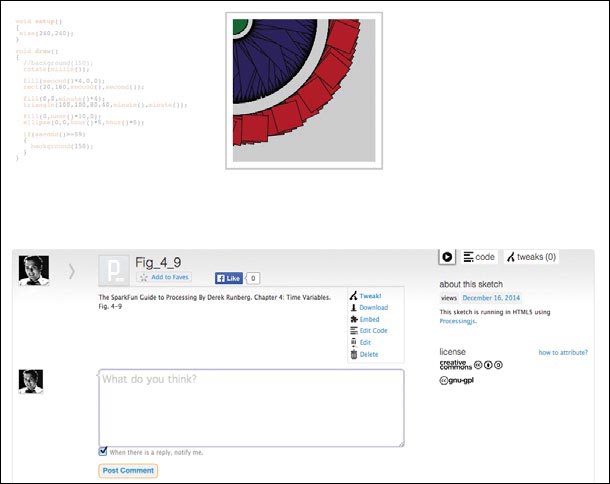
Fill out all of the content you want to include, click Save, and you should have a web-based version of your Processing application that you can share. Other OpenProcessing users can also fork your work, modify it, comment on it, and view it. Figure 4-13 shows what a sketch page looks like on OpenProcessing.

I touched on a few OpenProcessing basics to get you started with sharing and webifying your sketches, but I encourage you to explore this awesome tool further. Checking out other users’ code and tweaking it to see how it works is one of the best learning tools. Have fun!

FIGURE 4-12: Adding descriptive information to your sketch

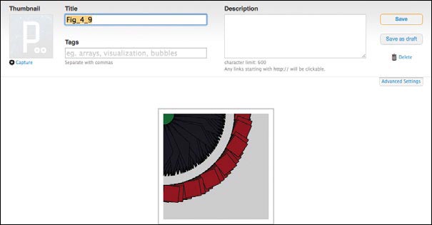
FIGURE 4-13: A basic sketch that changes color over time uploaded to OpenProcessing

TAKING IT FURTHER

A great way to take this project further would be to build time-based applications that are a little less creative but a bit more useful. You could incorporate the larger time-based variables by creating a calendar that draws something specific on a given day. Looking to the short term, you could also build a stopwatch for timing tasks, or you could even create a custom alarm clock by combining hour() and minute() with an if() statement! When you look not only at the system clock–based variables, but also millis(), the possibilities are endless.