
Image Processing with a Collage
Up to this point, you’ve used Processing as a canvas or digital collage of sorts, but you can also use it to manipulate images. Adding preexisting images to Processing lets you create multimedia projects that can include scans of hand-drawn illustrations, customized buttons, or even complete backgrounds.
Using photographs in Processing adds a few steps, but it is well worth the extra legwork. After you’ve added a photograph to your sketch, I’ll show you how to modify it with filters and change the tint.
FINDING AN IMAGE TO USE
If you’re like me, you probably have hundreds (if not thousands) of images on your computer, tablet, or smartphone. To add images to a Processing sketch, you need to do some preparation.
Start a new Processing sketch, and in the code window, click the Sketch drop-down menu and select Add File. This option should bring up the file dialog shown in Figure 6-1.
FIGURE 6-1: Find an image and place it in the data folder using the Add File option.
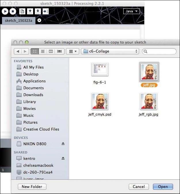
Find an image you want to use; this can be any .jpg, .bmp, or .png file. If your image has a crazy name, rename it something simple and descriptive. You’ll use that filename in your sketch, and long, random names leave opportunities for spelling errors. Once you’re happy with the filename, select the image and click Open.
NOTE
You can add images to your Processing sketch at any time, which allows for flexibility in your sketch design. However, if you know you’ll be using an image in your project, I suggest adding it at the very beginning, for simplicity and clarity.
Next, go back to the code window, click the Sketch drop-down menu, and select Show Sketch Folder. This folder is where your sketch resides when you save it, but it also includes all of the other assets that your sketch needs to run properly. There shouldn’t be much there right now, but your projects will have more files as they become more complicated.
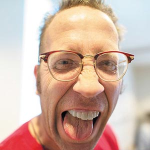
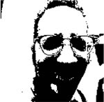
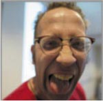
Open the folder named data, and you should see a copy of the image file you just added. I will be using the photograph of my friend Jeff in Figure 6-2. I named the file jeff.jpg. Take note of the file format (mine is .jpg, for example).
FIGURE 6-2: The original photo of my friend Jeff. It will look pretty different when I’m done!
THE PIMAGE DATA TYPE
You’ve seen a few different data types in this book already, including float, which is a number with a decimal point, and int (integer), which is a whole number. In this project, I introduce PImage, which is an advanced data type used for storing an image file.
PImage is considered advanced because when you create a PImage variable, you have to go through an extra step to initialize or assign an image to it. Here, I create a global variable (although a PImage can be a local variable as well) at the top of the sketch called img with a data type of PImage. Notice that I only create the variable and don’t initialize it with a value.
❶ img = loadImage(“jeff.jpg”);
}
To assign a value to img, you have to load your image ❶. Using the loadImage() function tells Processing to literally load, or pack, the img variable with every single pixel of the image.
To specify which image to pack, just pass loadImage() the filename as a string in quotes; I passed it "jeff.jpg". Since img is global, after you initialize it you can use the image it contains anywhere in your draw() loop or in any other function that follows the initialization.
USING YOUR IMAGE IN A SKETCH
Now that you have a variable holding your image, you need to put it to good use in the draw() loop by using the image() function. Think of an image as a rectangle that you can manipulate. The image() function accepts three parameters.
void draw()
{
image(img,100,100)
}
The first parameter is the image variable—in our case, img. The other two parameters indicate the location, (x,y), where you want to place the image origin. If you pass only these three parameters, the image adopts its original size. If you want to stretch and skew your image, you can add two more parameters, the width and height of the image, after the x- and y-coordinates.
When you use images in Processing, resolution really matters, because resolution is essentially the size of your image in pixels. Once you pull an image into Processing, you may notice that it is larger or smaller than you thought, and that can throw off your program. Be sure to check the original resolution of the images you are using under your image file properties before you use them in a project.
You should also think about aspect ratio—the ratio of height to width—when you choose images for your projects. If you are looking to scale or change the width or height of an image, that scaling will also stretch or contort the image. You may need to crop or edit some images to make them work for your project.
With that in mind, let’s explore the image modes available to you in Processing.
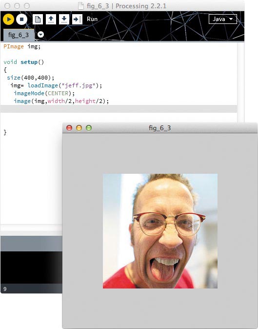
By default, the origin of an image is the same as that of a rectangle— the top-left corner. You can change this using a function called imageMode(). For example, if you want the origin to be the center of the image, you can pass the mode CENTER to imageMode(), and it will move the origin for you.
void draw()
{
imageMode(CENTER);
image(img,width/2,height/2);
}
Thanks to imageMode(), it takes only a couple of lines of code to place jeff.jpg in the center of my sketch window, as shown in Figure 6-3. To place the image using the image() function, I passed it img, which is the image I want to show, and the x- and y-coordinates of the center of the sketch (width/2 and height/2).
FIGURE 6-3: An image drawn in CENTER mode
These three modes are also options for rectangles and ellipses, courtesy of the rectMode() and ellipseMode() functions. Rectangles and ellipses have another available mode, too, called RADIUS.
The imageMode() function lets us choose from two other modes. Passing CORNER sets the origin back to the default (the top-left corner). Calling imageMode(CORNERS) will let you draw based on where you want the top-left and bottom-right corners of the image to fall in your sketch. In CORNERS mode, just pass image() the filename and two coordinates.
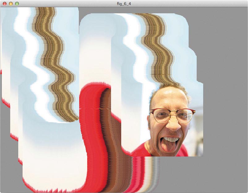
Since an image can be treated like a rectangle, you can even pass the mouseX and mouseY system variables to set its origin.
void draw()
{
❶ background(150);
imageMode(CENTER);
image(img,mouseX,mouseY);
}
You should now have an image that follows your mouse! Of course, just like any rectangle, an image leaves tracers behind by default, as shown in Figure 6-4. If you don’t want to see them, add a background() function ❶ to your draw() loop. Pretty cool, huh?
FIGURE 6-4: There are so many Jeffs! Get rid of that tracer so there’s only one.
You can translate, scale, and rotate your image just as you did for the basic shapes in previous chapters. All you need to do is set up a matrix in your draw() loop, and then you can transform the image as much as you want! For example, it’s always fun to play with scale.
void draw()
{
background(150);
imageMode(CENTER);
pushMatrix();
translate(width/2,height/2);//center image in your sketch
❶ scale(map(mouseX,0,width,.5,2));
image(img,0,0);
popMatrix();
}
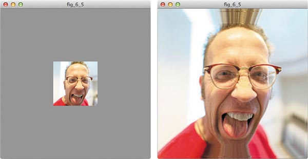
Notice that I’ve passed a mapped value of mouseX to scale() ❶. Processing’s map() function maps a value onto a different range of values. Here, I’ve told Processing to map the range of mouseX—which would normally be from 0 to the width of your sketch—to values ranging from .5 to 2, resulting in scales from 50 to 200 percent. This should turn your mouse movements into a zoom control, as shown in Figure 6-5.
FIGURE 6-5: The farther you move the mouse along the x-axis, the more you’ll zoom in on your image.
Now that you’ve played with one image, let’s up the ante and move on to this chapter’s project. You can add as many pictures as you want to your Processing sketch, and you can also assemble them into a collage, just as you did with the basic shapes to create a holiday image in Project 2. I’ll show you a few other useful tools on the way to finishing your photo collage, too.
A PHOTO COLLAGE
The main reason for using matrices is so you can group individual or sets of objects together and manipulate them independently from the rest of your sketch. In a photo collage, you may want to modify a specific image or group of images while keeping others intact. I recommend placing each image on its own matrix so that you can work with it freely. If you want to apply the same effects to multiple images, you can place them within the same matrix, but at some point you may want to separate them.
NOTE
You can download the images I used for this project from https://learn.sparkfun.com/about/. Use those images for this collage if you’d like, but to make it your own, search your library for six that have the same resolution as mine (200 pixels by 200 pixels) and use those instead!
I’m going to use images of my other teammates at SparkFun to create a photo collage in Processing. You could create a scrapbook page from your last family trip, a collage of scans of your favorite doodles, or, really, anything you can imagine.
Multiple Images
To use multiple images in a project, first you need to add those images to your data folder. Click Sketch ![]() Add File and add the
Add File and add the
first new file to your data folder, and then repeat those steps until you’ve added all the images you need. When you’re finished, I recommend clicking Sketch ![]() Show Sketch Folder to access the data folder and changing the names of the images to something simple.
Show Sketch Folder to access the data folder and changing the names of the images to something simple.
Next, create a variable for each image, with the data type PImage. Since you have more than one image, use descriptive variable names to keep them all straight. I named each image variable after the person in the photo I plan to load into that variable.
PImage jeff;
PImage amanda;
PImage lindsay;
PImage ben;
PImage brian;
PImage angela;
void setup()
{
size(1000,800);
amanda = loadImage("amanda.png");
lindsay = loadImage("lindsay.png");
ben = loadImage("ben.png");
brian = loadImage("brian.png");
angela = loadImage("angela.png");
}
void draw()
{
❷ image(jeff,20,20);
image(amanda,600,400);
image(lindsay,300,20);
image(ben,20,400);
image(brian,600,20);
image(angela,300,400);
}
The final step of preparing your images is loading the files to variables. Call the loadImage() function ❶ inside the setup() code and assign the image files to the variables you created at the top of your sketch. Now you can draw them onto your sketch window, as shown in Figure 6-6, by calling the image() function ❷ and supplying your desired coordinates.
FIGURE 6-6: Placing multiple images on a sketch
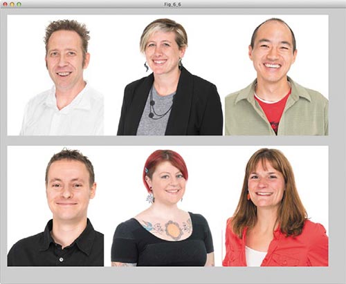
I’m going to continue using these images throughout the project, so for reference, in Figure 6-6 the filenames are (clockwise from top left) jeff.png, lindsay.png, brian.png, amanda.png, angela.png, and ben.png.
If you know where you want your images within your sketch and you’re not looking to move them around or to transform them in any way, you’re finished. But you’re probably looking to do more than just place your images in clean, straight rows. This is where the strength of the matrix comes in.
Returning to the Matrix
Whenever you’re working with multiple images, I recommend getting into the habit of using matrices. You can give each image its own matrix and then manipulate those matrices independently of one another. As an example, I’m going to tweak the draw() loop from the previous section to get each image ready for using a matrix.
void draw()
{
pushMatrix();
translate(20,20);
image(jeff,0,0);
popMatrix();
pushMatrix();
❶ translate(300,20);
❷ image(lindsay,0,0);
popMatrix();
pushMatrix();
translate(300,400);
image(angela,0,0);
popMatrix();
pushMatrix();
translate(600,400);
image(amanda,0,0);
popMatrix();
pushMatrix();
translate(600,20);
image(brian,0,0);
popMatrix();
translate(20,400);
image(ben,0,0);
popMatrix();
}
All you have to do is place each image in its own matrix and translate that matrix to the position at which you were drawing the image before. Remember how each matrix has its own origin? I placed all of the images at (0,0) and moved the matrices—not the images. To move the matrices, give each a translate() function at the top. For example, I drew the lindsay picture at (300,20) originally, but here, I translate the matrix to that point ❶ and draw the image at the origin of its matrix ❷, which is at (300,20). Follow the same pattern for your own collage, and when you click Run, all of the image locations should be the same as before.
Now you can manipulate each image within its matrix. So to move one of your images, you’ll use the translate() function to move the matrix rather than the image itself. This may seem like a lot of work, but trust me: it’s worth the effort. Now, let’s make your collage a bit more interesting.
NOTE
In my setup code, I didn’t set an imageMode(), so if you’re using CENTER, your sketch may act differently.
Scattered Photos
Straight and true images are a little boring. Since each image is in its own matrix you can add some transformation functions to give your sketch a little more depth and interest. You can also rotate, scale, and otherwise manipulate each image as you see fit once they’re all inside matrices. Give it a try! Mix up that perfectly aligned collage to make the pictures look like they’ve been strewn on the sketch.
PImage jeff;
PImage amanda;
PImage lindsay;
PImage ben;
PImage brian;
PImage angela;
void setup()
{
size(1000,800);
jeff = loadImage("jeff.png");
amanda = loadImage("amanda.png");
lindsay = loadImage("lindsay.png");
ben = loadImage("ben.png");
brian = loadImage("brian.png");
angela = loadImage("angela.png");
background(200,0,200);//purple background
imageMode(CENTER);
}
void draw()
{
pushMatrix();
translate(500,20);
rotate(1.6);
scale(1.5);
image(angela,0,0);
popMatrix();
pushMatrix();
translate(200,200);
rotate(.5);
image(jeff,0,0);
popMatrix();
pushMatrix();
translate(600,600);
rotate(1.3);
scale(1.5);
image(amanda,0,0);
popMatrix();
pushMatrix();
translate(150,500);
rotate(.15);
image(brian,0,0);
popMatrix();
pushMatrix();
translate(800,200);
rotate(-1);
image(ben,0,0);
popMatrix();
pushMatrix();
translate(500,400);
scale(.75);
rotate(.2);
image(lindsay,0,0);
popMatrix();
}
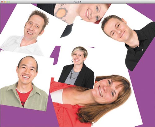
In this version of my collage code, I added the imageMode() and background() functions to the setup() section. In the draw() loop, I scaled or rotated some images, with the scale() and rotate() functions, respectively. These changes offer more appeal than just static images, as you can see in Figure 6-7.
FIGURE 6-7: This collage is much more dynamic.
It’s great that you can handle multiple images and modify them individually using the transformation functions you learned in previous chapters, but now I’ll introduce you to a few image-specific modifiers so you can give your collage even more creative depth.
APPLYING TINTS
First we’ll explore the tint() function, which allows you to add a colored tint to an image. tint() is a modifier, so just like fill() or stroke(), it must be placed before the image that you’re tinting.
Changing the tint of your image is as simple as passing tint() red, green, and blue values, but I think the coolest part of the tint() function is that it allows you to set the transparency value of the image as well. To set the transparency, pass a fourth argument ranging from 0 to 255, where 0 is completely invisible and 255 is completely opaque, or solid.
Try it out now! In my collage, I added a tint to all of my images except the one of Lindsay, which I explicitly removed the tint from with noTint(), as shown in Listing 6-1.
LISTING 6-1: Applying tints to the collage
PImage jeff;
PImage amanda;
PImage lindsay;
PImage ben;
PImage brian;
PImage angela;
void setup()
{
size(1000,800);
jeff = loadImage("jeff.png");
amanda = loadImage("amanda.png");
lindsay = loadImage("lindsay.png");
ben = loadImage("ben.png");
brian = loadImage("brian.png");
angela = loadImage("angela.png");
background(200,0,200);
imageMode(CENTER);
}
void draw()
{
Background(150);
pushMatrix();
translate(500,20);
rotate(1.6);
scale(1.5);
❶ tint(second() * 4,second() * 4,second() * 4);
image(angela,0,0);
popMatrix();
pushMatrix();
translate(200,200);
rotate(.5);
❷ tint(255,mouseY/4);
image(jeff,0,0);
popMatrix();
translate(600,600);
rotate(1.3);
scale(1.5);
tint(100,150,0);
image(amanda,0,0);
popMatrix();
pushMatrix();
translate(150,500);
rotate(.15);
❸ tint(mouseX/4,mouseY/4,0);
image(brian,0,0);
popMatrix();
pushMatrix();
translate(800,200);
rotate(-1);
❹ tint(255,255,255,mouseX/4);
image(ben,0,0);
popMatrix();
pushMatrix();
translate(500,400);
scale(.75);
rotate(.2);
noTint();
image(lindsay,0,0);
popMatrix();
}
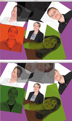
Try adding variables to the tint() function so that you can make your work feel interactive. The tint for Angela’s image ❶ changes color over time, and the images of Jeff ❷, Brian ❸, and Ben ❹ all change if you move the mouse. The image of Ben fades in and out of the foreground depending on the mouseX value, Brian changes color depending on both mouse positions, and Jeff actually changes transparency, but not color. (If you don’t look carefully at the beginning of the sketch, you may miss the change in Jeff’s picture!) Check out the result in Figure 6-8.
FIGURE 6-8: My photo collage with the tint() function added. You can see the difference between the two before and after I moved the mouse around.
NOTE
I’ll explain the basics of the filter() function, but if you’re looking for more advanced filtering options, the examples and tutorials at Processing.org are a great place to explore.
FILTER BASICS
You can accomplish a lot with the tint() function, but you can extend image manipulation and modification even further by using the filter() function, which has filters similar to those available in photo editing software.
The filter() function doesn’t work exactly like other image modifiers. The filter is placed over the image, like a mask that you’re looking through. The filter() function also requires a filter name, rather than numeric values. Table 6-1 lists Processing’s seven default filters along with examples of what each does to an image. To compare against the original image, flip back to the photo in Figure 6-1.
TABLE 6-1: Processing’s default filters
| FILTER | RESULT |
| filter(THRESHOLD); (Range: 0–1) |
 |
| filter(GRAY); |  |
| filter(INVERT); | 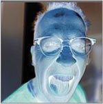 |
| filter(POSTERIZE,4); (Range: 2–255) |
 |
| filter(BLUR,1); (Range: ≥1) |
 |
| filter(ERODE); | 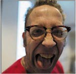 |
| filter(DILATE); | 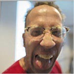 |
A few of these filters are stand-alone, meaning there is only one setting. A few of them—THRESHOLD, POSTERIZE, and BLUR—allow you to pass an additional value to change a setting or intensity. For those, I have provided the range of numbers that you can pass to the filter.
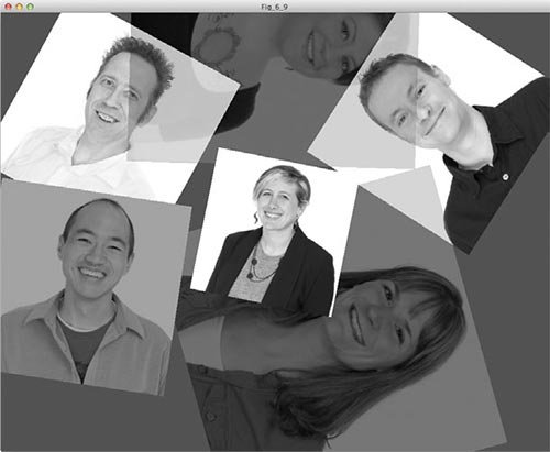
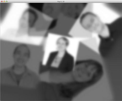
There are two different techniques for applying a filter. The simplest way is to place the filter over the entire sketch. This is helpful when you want to use a general filter, such as a blur, or when you want to make everything grayscale. For example, at the very end of your photo collage, add the line filter(GRAY); to produce a grayscale sketch like the one in Figure 6-9.
FIGURE 6-9: Even after I added tints to several images, the filter still made everything grayscale.
You can also stack image filters by adding a second filter function after the first one. For example, add a BLUR filter with a level of 7 after your initial GRAY filter:
filter(GRAY);
filter(BLUR,7);
This combination should produce a blurry black-and-white image like the one in Figure 6-10.
FIGURE 6-10: Pass larger second arguments to filter() to increase the blurriness.
To apply a filter to a single image rather than to the whole sketch, you’ll need to use a different approach that breaks from how we’ve been writing code up to this point. But before we dive in to that, I’ll explain a little more about advanced data types.
Advanced data types have two faces. The first, and the most apparent, is that they’re data types, just like an int or a float. But unlike a variable with an int or float value, variables that have advanced data types like PImage are considered objects. In object-oriented programming (OOP), you create an object, which is an instance of a class. A class has certain properties that it passes on to every object of that class type.
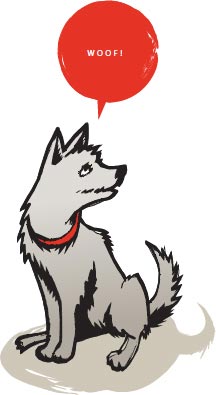
Let’s go through an example of how classes and objects work. Start by thinking about a dog. A dog has a weight, a color, and other properties; dogs also greet you when you come home and sit and stand on command. Those aspects form a template that applies to all dogs, and a class is like that template. In a dog class, properties like weight and color are called fields; while actions like greet() or sit() can be stored as methods, which are just functions defined in a class.
Now, consider an adorable dog named Fluffy. Fluffy is a specific instance of the dog class, so she’s an object. Figure 6-11 shows some fields and methods that our Fluffy object might have if she were part of a program.
FIGURE 6-11: Fluffy is an instance of dog, so she has the same fields and methods as any other dog object.
object: Fluffy
class: dog
fields:
weight = 40 lbs
color = "brown"
isSitting = true
methods:
void greet()
{
println("Woof!")
}
void sit()
{
isSitting = true;
}
void stand()
{
isSitting = false;
}
Fluffy displays a friendly “Woof!" string when you call her greet() method. Fluffy is also currently sitting because isSitting is true; if you called the stand() method on Fluffy, she’d stand up and isSitting would change to false.
In Processing, photos can take actions and change fields based on your commands, too. They can change filters, width, height, and so on. Those actions would be methods on a photo object. PImage is a built-in class, and its preset methods actually include the filter() function you’ve already encountered.
You don’t need to take a deep dive into OOP to complete this project, but if you’re curious, check out the “More on Object-Oriented Programming” box.
MORE ON OBJECT-ORIENTED PROGRAMMING
You can think of classes and their functions in terms of this simplified hierarchy:
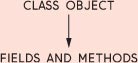
The class object at the top has a number of fields and methods. For example, think about Fluffy from Figure 6-11. She is an instance of the dog class, and all dogs have fields like color, weight, and breed. Once you start playing with a dog, it also has a number of methods: you can tell it to greet, for example.
There is a difference between fields and methods, though. Fields return information about the object; examples in Processing include width and height. On the other hand, a method, such as filter() or save(), is a procedure to do something. You’ve already used some of the methods and fields of the PImage class, but a few more are shown in this table:
| METHODS | FIELDS |
| save() | width |
| resize() | height |
| copy() | pixels[] |
| blend() | |
| get() | |
| set() |
One major visual difference between fields and methods is that methods have parentheses and fields are usually just keywords. Play around with these fields and methods to see what you can do with the PImage class!
When you think about your images as objects, you can start to consider different aspects of the image that you can either use as variables or change. For example, the filter of an image is something that you can change by calling a method on an image object:
lindsay.filter();
For this example, I used an image of Lindsay stored in a PImage object named lindsay. I then applied the filter() method to lindsay by adding a period after the object name followed by a call to the method.
Follow the same rule any time you want to apply one of the class’s methods to any object of that class. But a word of warning: you can’t just use any old function in this way! The function must actually be a method, which means it must exist as part of the object’s class. I can apply filter() to lindsay because lindsay is an instance of the PImage class, which includes that function.
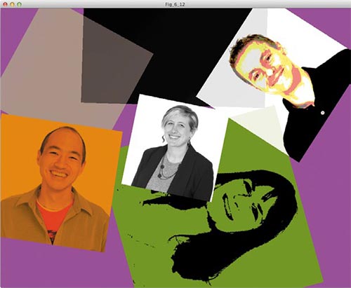
This object-oriented approach is what allows you to apply a specific filter to a specific image, rather than applying it to all of the images in your sketch. If you want to apply specific filters to certain images, add the functions in the setup() of your sketch rather than in the draw() loop. For example, add the following object-oriented function calls to your setup() function from Listing 6-1.
jeff.filter(BLUR,7);
lindsay.filter(GRAY);
ben.filter(POSTERIZE,3);
angela.filter(ERODE);
brian.filter(INVERT);
amanda.filter(THRESHOLD,.8);
NOTE
I placed the individual filter functions in setup() because some of them act oddly when placed in the draw() loop. For example, the INVERT filter will alternate between being inverted and not. You can play around with where you place these filter functions to get the effect you’re looking for, but for now I am placing them in setup().
Working with the same code and images as in previous examples, I gave each image its own filter by calling the image object followed by a period and then the filter() function that I wanted to apply to that image.
Adding those filters produces the sketch in Figure 6-12, where you can see that each image has its own individual filter.
If you try adding those filters in the draw() loop, each layer that you add below an image visually stacks on top of the other in your sketch. This means that the first image would have all of the subsequent filters applied to it. That would be quite a mess! Fortunately, if you do want all images to have some filter in common, even after each image has its own filter, you can still apply a full filter within your draw() loop as well.
FIGURE 6-12: Thanks to individual filters, each image looks very different from the others.
Filters and the tint() function are great ways to add interest and creativity to your images and your sketch as a whole. A lot of things that are normally accomplished with high-level, expensive editing software can be accomplished in Processing, and in much more creative and interactive ways.
TAKING IT FURTHER
Now that you’ve played around with changing filters and changing image parameters with variables, you can do some really cool work with images and Processing. Try experimenting with not only photographs but also hand-drawn characters. Just scan them into your computer and add them to your sketch! Processing is a great way to create basic animations and even presentations.
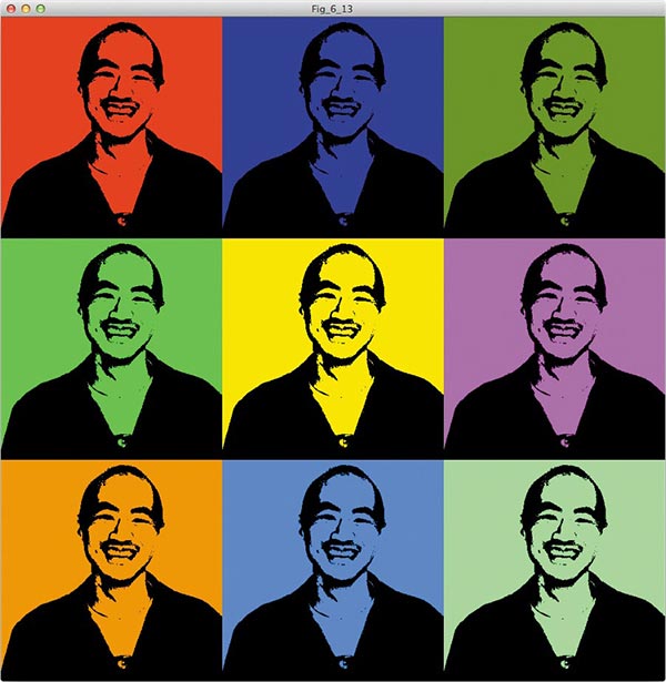
To get more practice with tints and filters, try creating an image of yourself or someone else in the spirit of Andy Warhol. Just make a 3×3 grid of the same image, and apply different filters and tints to each image to create variations on the original. The cool thing is that you only need to include a single image file in your sketch; you just use the image function nine times over with different filters. The end product will be more interesting than the sum of its parts. For a final inspiration, Figure 6-13 shows a quick example I created.
FIGURE 6-13: My Warhol-inspired portrait of Brian
And here is some code to get you started:
PImage brian;
void setup()
{
brian = loadImage("brian.jpg");
brian.filter(THRESHOLD,.88);
size(900,900);
}
void draw()
{
tint(255,0,0);
image(brian,0,0,300,300);
image(brian,300,0,300,300);
tint(0,255,0);
image(brian,600,0,300,300);
}
I applied the THRESHOLD filter to the image in the setup() and then tinted each image individually. This code is only for the first row, so you’ll have to finish the other rows yourself. Choose an image of your own, and use this method to create a Warhol-inspired painting!