Chapter

Introduction

The central theme in this book is to investigate and explore various properties of the class of totally nonnegative matrices.

At first it may appear that the notion of total positivity is artificial; however, this class of matrices arises in a variety of important applications. For example, totally positive (or nonnegative) matrices arise in statistics (see [GM96, Goo86, Hei94]), mathematical biology (see [GM96]), combinatorics (see [BFZ96, Bre95, Gar96, Pen98]), dynamics (see [GK02]), approximation theory (see [GM96, Pri68, CP94B]), operator theory (see [Sob75]), and geometry (see [Stu88]). Historically, the theory of totally positive matrices originated from the pioneering work of Gantmacher and Krein ([GK60]) and was elegantly brought together in a revised version of their original monograph [GK02]). Also, under the influence of I. Schoenberg (see, for example, [Sch30]), Karlin published an influential treatise, Total Positivity ([Kar68]), which mostly concerns totally positive kernels but also deals with the discrete version, totally positive matrices. Since then there has been a considerable amount of work accomplished on total positivity, some of which is contained in the exceptional survey paper by T. Ando ([And87]). Two more recent survey papers have appeared ([Fal01] [Hog07, Chap. 21]) and both take the point of view of bidiagonal factorizations of totally nonnegative matrices.

Before we continue, as mentioned in the Preface, we issue here a word of warning. In the existing literature, the terminology used is not always consistent with what is presented above. Elsewhere in the literature the term totally positive (see below) corresponds to “strictly totally positive” (see, for example, the text [Kar68]) and the term totally nonnegative defined here sometimes corresponds to “totally positive” (as in some of the papers in [GM96]).

0.0 DEFINITIONS AND NOTATION

The set of all m-by-n matrices with entries from a field will be denoted by . If , the set of all real numbers, then we may shorten this notation to M_m,n. Our matrices will, for the most part, be real entried. In the case m=n, the matrices are square and or M_m,n will be shortened to or M_n. For , the notation will indicate that the entries of A are , for and . The transpose of a matrix A will be denoted by A^T.

For , , and , of A lying in rows indexed by α and columns indexed by β will be denoted by . Similarly, is the submatrix obtained from A by deleting the rows indexed by α and columns indexed by β. Throughout the book, we let α^c denote the complement of the index set α. So, in particular, . If and α=β, then the principal submatrix A[α, α] is abbreviated to A[α], and the complementary principal submatrix is A(α). On the other hand, if , then the submatrix A[α, β] is referred to as a nonprincipal submatrix of A. In the special case when with , we refer to the principal submatrix A[α] as a leading principal submatrix. In the same manner, for an n-vector , x[α] denotes the entries of x in the positions indexed by α and x(α) denotes the complementary vector. If , then we let denote the n-by-n diagonal matrix with main diagonal entries x_i. For brevity, we often denote the sets and by M and N, respectively.

A minor in a given matrix A is by definition the determinant of a (square) submatrix of . Here and throughout, denotes the determinant of a square matrix. For example, if , the minor detA[α, β] may also be denoted by A_{α, β}, and the principal minor (if A is square) detA[α] may be abbreviated to A_α.

We are interested here in those matrices with all minors positive (nonnegative) and, occasionally, with all minors A_{α, β}, with positive (nonnegative). The former are called the totally positive (totally nonnegative) matrices and are denoted by TP (TN); we denote the latter as TP_k (TN_k). TP (TN) is used both as an abbreviation and as a name of a set. The reader should consult [HJ85, HJ91] or any other standard reference on matrix theory for standard notation and terminology not defined herein. In terms of compounds, TP_k, for example, simply means that the first through the kth compounds are entry-wise positive.

Several related classes of matrices are both of independent interest and useful in developing the theory of TP (TN) matrices. We give our notation for those classes here; we continue to use the subscript k to denote a requirement made on all minors of no more than k rows. No subscript indicates that the requirement is made on all minors. Each class is defined irrespective of the m and n in M_m,n, except that a subscript k makes sense only for .

By InTN (InTN_k), we denote the square and invertible TN matrices (TN_k matrices), and by IrTN (IrTN_k), we mean the square and irreducible TN matrices (TN_k matrices). The intersection of these two classes is denoted by IITN (IITN_k); this class is also referred to as the oscillatory matrices [GK60], which are defined as those TN matrices with a TP integral power. The equivalence will be demonstrated in Chapter 2. We may also use the symbol OSC to denote oscillatory matrices.

A TN (TN_k) matrix may have a zero line (row or column), which often leads to an exception to convenient statements. So we denote TN (TN_k) matrices with no zero lines as TN’ (TN_k′).

A square, triangular matrix cannot be TP, but one that is TN and has all its minors positive unless they are identically 0 because only of the triangular structure is called triangular TP; these are denoted by ΔTP. Similarly, ΔTN denotes the triangular, TN matrices. An adjective “upper” or “lower” denotes the form of triangularity. Finally, the positive diagonal matrices () are the intersections of upper ΔTP and lower ΔTP matrices, and thus are InTN.

For convenience of reference we present these classes in tabular form in Table 1. Note: Omission of subscript k means all minors.

Table 1: Various Classes of Matrices of Interest

The ith standard basis vector is the n-vector whose only nonzero entry occurs in the ith component and that entry is a one, and is denoted by e_i; the (i,j)th standard basis matrix, the m-by-n matrix whose only nonzero entry is in the (i,j)th position and this entry is a one, will be denoted by E_ij.

Observe that if m=n, then . We also let e denote the n-vector consisting of all ones (the size of e will be determined from the context). Finally, we let J_m,n () and I_n denote the m-by-n matrix of all ones and the n-by-n identity matrix, respectively. The subscript is dropped when the sizes of these matrices is clear from the context.

0.1 JACOBI MATRICES AND OTHER EXAMPLES OF TN MATRICES

An n-by-n matrix is called a diagonal matrix if whenever . For example,

is a 4-by-4 diagonal matrix. We may also write A as .

An n-by-n matrix is referred to as a tridiagonal matrix if whenever . For example,

is a 4-by-4 tridiagonal matrix. The entries of that lie in positions are referred to as the superdiagonal, and the entries of A in positions are called subdiagonal.

Hence a matrix is tridiagonal if the only nonzero entries of A are contained on its sub-, main, and superdiagonal.

Tridiagonal matrices are perhaps one of the most studied classes of matrices. Much of the reason for this is that many algorithms in linear algebra require significantly less computational labor when they are applied to tridiagonal matrices. Some elementary examples include

(1) eigenvalues,

(2) solving linear systems,

(3) LU factorization,

(4) evaluating determinants.

For instance, the determinant of a tridiagonal matrix can be evaluated by solving the recursive equation

(1)

Equation (1) is a simple consequence of the Laplace expansion of det A along row (or column) 1. Furthermore, both and are (smaller sized) tridiagonal matrices.

The recursive relation (1) also ties the eigenvalues of a (symmetric) tridiagonal matrix to certain orthogonal polynomials (Chebyshev), as the characteristic polynomials of A and its principal submatrices also satisfy a relation like (1). In addition, (1) arises in the Runge-Kutta methods for solving partial differential equations.

Suppose the tridiagonal matrix A has the form

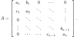(2)

Observe that a tridiagonal matrix A in the form (2) is called symmetric if , and is called irreducible if both and , for .

An n-by-n matrix is called a P₀-matrix if all its principal minors are nonnegative. We let P₀ denote the class of all P₀-matrices. Furthermore, an n-by-n matrix is called a P-matrix if all its principal minors are positive. We let P denote the class of all P-matrices.

Suppose A in (2) is an irreducible nonnegative tridiagonal matrix. If , where , then A is a P₀-matrix. To verify this claim we need the following fact. If A is tridiagonal, then the principal submatrix can be written as , where ⊕ denotes direct sum. In particular,

Hence to calculate any principal minor of a tridiagonal matrix, it is enough to compute principal minors based on associated contiguous index sets. Moreover, any principal submatrix of a tridiagonal matrix based on contiguous index sets is again a tridiagonal matrix. To verify that any tridiagonal of the form (2) that is nonnegative, irreducible and satisfies (row diagonal dominance) is a P₀-matrix, it is sufficient, by induction, to verify that .

Consider the case n = 3. Then by (1),

In addition, since it follows from (1) that

(3)

Consider the general case and let A’ be the n-by-n matrix obtained from A by using an elementary row operation to eliminate c₁. Then, as ,

Observe that this matrix is an irreducible, nonnegative tridiagonal matrix that still satisfies the row dominance relation and hence by induction has a positive determinant. Thus .

Furthermore, we note that by (1) we have

So, if a nonnegative, irreducible tridiagonal matrix satisfies the simple dominance relation it is a P₀-matrix. In fact, even more is true.

Since tridiagonal matrices satisfy whenever it is a simple consequence that

whenever there exists an such that .

Furthermore, if is any submatrix of A that satisfies , then is a product of principal minors and nonprincipal minors, where the principal minors are based on contiguous index sets and the nonprincipal minors are simply entries from the super- and/or subdiagonal.

For example, suppose A is a 10-by-10 tridiagonal matrix of the form in (2).

Then

Consequently, any irreducible, nonnegative tridiagonal matrix that satisfies the condition has all its minors nonnegative.

We remark here that the irreducibility assumption was needed for convenience only. If the tridiagonal matrix is reducible, then we simply concentrate on the direct summands and apply the same arguments as above.

The upshot of the previous discussion is that if A is a nonnegative tridiagonal matrix that also satisfies , then A is TN.

In the pivotal monograph [GK60], the chapter on oscillatory matrices began by introducing a class of tridiagonal matrices the authors called Jacobi matrices. An n-by-n matrix is a Jacobi matrix if is a tridiagonal matrix of the form

Further, is called a normal Jacobi matrix if, in addition, . Jacobi matrices were of interest to Gantmacher and Krein for at least two reasons. First, many of the fundamental properties of general oscillatory matrices can be obtained by an examination of analogous properties of Jacobi matrices. Second Jacobi matrices are among the basic types of matrices that arose from studying the oscillatory properties of an elastic segmental continuum (no supports between the endpoints) under small transverse oscillations.

One of the first things that we observe about Jacobi matrices is that they are not TN or even entrywise nonnegative. However, they are not that far off, as we shall see in the next result.

The following result on the eigenvalues of a tridiagonal matrix is well known, although we present a proof here for completeness.

Lemma 0.1.1 Let T be an n-by-n tridiagonal matrix in the form

(4)

If for , then the eigenvalues of T are real and have algebraic multiplicity one (i.e., are simple). Moreover, T is similar (via a positive diagonal matrix) to a symmetric nonnegative tridiagonal matrix.

Proof. Let be the n-by-n diagonal matrix where , and for k > 1, . Then it is readily verified that

Since is symmetric and T and have the same eigenvalues, this implies that the eigenvalues of T are real. Suppose λ is an eigenvalue of T. Then is also of the form (4). If the first row and last column of are deleted, then the resulting matrix is an (n-1)-by-(n-1) upper triangular matrix with no zero entries on its main diagonal, since , for . Hence this submatrix has rank n-1. It follows that has rank at least n-1. However, has rank at most n-1 since λ is an eigenvalue of T. So by definition λ has geometric multiplicity one. This completes the proof, as is also a nonnegative matrix.

A diagonal matrix is called a signature matrix if all its diagonal entries are ± 1. Furthermore, two n-by-n matrices A and B are said to be signature similar if , where S is a signature matrix. It is not difficult to verify that a normal Jacobi matrix is signature similar to a nonnegative tridiagonal matrix. Furthermore, the eigenvalues of a normal Jacobi matrix are real and distinct.

Observe that if an irreducible normal Jacobi matrix satisfies the dominance condition (), then it is similar to a symmetric TN tridiagonal matrix. In particular (since a symmetric TN matrix is an example of a positive semidefinite matrix [HJ85]), the eigenvalues are nonnegative and distinct by Lemma 0.1.1.

Moreover, if the above normal Jacobi matrix is also invertible, then the eigenvalues are positive and distinct.

Since the eigenvalues are distinct, each eigenvalue has exactly one eigenvector (up to scalar multiple), and these (unique) eigenvectors satisfy many more interesting “sign” properties.

Let

Given above, define

Recall that the functions D_k satisfy the recurrence relation

(5)

for . Evidently,

and so on.

A key observation that needs to be made is the following:

“When vanishes , the polynomials and differ from zero and have opposite sign.”

Suppose that, for some k, , this property fails. That is, for fixed ,

Go back to the recurrence relation (5), and notice that if the above inequalities hold, then

Consequently, for all . But then observe

which implies . Now we arrive at a contradiction since

and

Since we know that the roots are real and distinct, when λ passes through a root of , the product must reverse sign from + to −. A consequence of this is that the roots of successive D_k’s strictly interlace. Using this interlacing property we can establish the following simple but very important property of the functions . Between each two adjacent roots of the polynomial lies exactly one root of the polynomial (that is, the roots interlace).

Observation: The sequence

has j-1 sign changes when where are the distinct eigenvalues of .

Further note that and so it follows that .

Finally, we come to the coordinates of the eigenvectors of . Assume for the moment that for each i, and (for simplicity’s sake).

Suppose

is an eigenvector of corresponding to the eigenvalue λ. Then examining the vector equation yields the system of equations

Since , it follows that ; hence the first n-1 equations are linearly independent, and the nth equation is a linear combination of the previous n-1.

Looking more closely at the first n - 1 equations we arrive at the relation

Hence the coordinates of x satisfy the same relation as .

Hence , constant. Thus, since at the sequence has exactly j - 1 sign changes, it follows that the eigenvector corresponding to has exactly j - 1 sign changes. The interlacing of sign changes in the eigenvectors follows as well.

We close with a remark that offers a nice connection between tridiagonal TN matrices and a certain type of additive closure (a property not enjoyed by general TN matrices). Suppose A is a TN matrix. Then a simple examination of the 2-by-2 minors of A involving exactly one main diagonal entry will be enough to verify the following statement. The matrix A is tridiagonal if and only if A+D is TN for all positive diagonal matrices D. This result also brings out the fact that tridiagonal P₀ matrices are, in fact, TN.

0.1.1 Other Examples of TN Matrices

In the previous subsection we demonstrated that any entrywise nonnegative tridiagonal P₀-matrix was in fact TN. Other consequences include (1) an entry-wise nonnegative invertible P₀ tridiagonal matrix is both InTN and a P-matrix, and (2) an entrywise nonnegative invertible P₀ tridiagonal matrix is IITN and hence oscillatory.

From tridiagonal matrices, it is natural to consider their inverses as another example class of InTN matrices.

Example 0.1.2 (Inverses of tridiagonal matrices) Let T be an InTN tridiagonal matrix. Then is another InTN matrix. For example, if

then

In fact, note that the matrix

is the inverse of a tridiagonal matrix and is also InTN.

We also acknowledge that these matrices are referred to as “single-pair matrices” in [GK60, pp. 79–80], are very much related to “Green’s matrices” in [Kar68, pp. 110–112], and are connected with “matrices of type D” found in [Mar70].

Tridiagonal and inverse tridiagonal TN matrices have appeared in numerous places throughout mathematics. One instance is the case of the Cayley transform. Let such that I+A is invertible. The Cayley transform of A, denoted by , is defined to be

The Cayley transform was defined in 1846 by A. Cayley. He proved that if A is skew-Hermitian, then is unitary, and conversely, provided, of course, that exists. This feature is useful, for example, in solving matrix equations subject to the solution being unitary by transforming them into equations for skew-Hermitian matrices. One other important property of the Cayley transform is that it can be viewed as an extension to matrices of the conformal mapping

from the complex plane into itself. In [FT02] the following result was proved connecting essentially nonnegative tridiagonal matrices and TN matrices. Recall that a matrix is called essentially nonnegative if all its off-diagonal entries are nonnegative.

Theorem 0.1.3 Let be an irreducible matrix. Then A is an essentially nonnegative tridiagonal matrix with for all eigenvalues λ of A if and only if I+A and are TN matrices. In particular, is a factorization into TN matrices.

Proof. To verify necessity, observe that if I+A is TN, then A is certainly essentially nonnegative. Also, since is TN, it follows that I-A is invertible and has the checkerboard sign pattern (i.e., the sign of its (i,j)th entry is ). Hence and for all , and since A is irreducible and I+A is TN, for . That is, A is tridiagonal. The remaining conclusion now readily follows.

For the converse, if A is an essentially nonnegative irreducible tridiagonal matrix with for all eigenvalues λ of A, then I+A is a nonnegative tridiagonal P-matrix and thus totally nonnegative (see previous section). Similarly, I-A is a tridiagonal M-matrix since for all eigenvalues λ of A (recall that an n-by-n P-matrix is called an M-matrix if all off-diagonal entries are nonpositive), and hence is TN (this follows from the remarks in the previous section). Since TN matrices are closed under multiplication, is TN.

A natural question arising from Theorem 0.1.3 is whether in every factorization of a totally nonnegative matrix the factors and are TN. We conclude with an example showing that neither of these factors need be TN.

Consider the TN matrix

and consider . Then , where neither

is TN.

Example 0.1.4 (Vandermonde) Vandermonde matrices have been an example class of matrices that have garnered much interest for some time. In many respects it is not surprising that certain Vandermonde matrices are TP (see Chapter 1 for more discussion). For n real numbers , the Vandermonde matrix is defined to be

and is a TP matrix (see [GK60, p. 111]). Recall the classical determinantal formula,

which is positive whenever .

The reader is also encouraged to consult [GK60] for similar notions involving generalized Vandermonde matrices. Totally positive Vandermonde matrices were also treated in the survey paper on bidiagonal factorizations of TN matrices [Fal01], which we discuss further below.

It is really quite remarkable that the inequalities are actually sufficient to guarantee that all minors of V above are positive. Indeed, any 2-by-2 submatrix of V has the form

where , i<j, , and . Since , it follows that . Hence, in this case, A is TP. For an arbitrary k-by-k submatrix of V, consider the following argument, which is similar to that given in [GK60] and in [Fal01]. Any k-by-k submatrix of is of the form , where , , , and . Let be a real polynomial. Descartes’s rule of signs ensures that the number of positive real roots of f(x) does not exceed the number of sign changes among the coefficients , so f(x) has at most k-1 positive real roots. Therefore, the system of equations

has only the trivial solution , so .

To establish that , we use induction on the size of A. We know this to be true when the size of A is 2, so assume whenever the size of A is at most k-1. Let be k-by-k, in which , , , and . Then expanding det A along the last row gives

But , where , so the induction hypothesis ensures that . Thus as , so . The conclusion is that is TP whenever .

Example 0.1.5 (Cauchy matrix) An n-by-n matrix is called a Cauchy matrix if the entries of C are given by

where and are two sequences of real numbers (chosen accordingly so that c_ij is well defined). A Cauchy matrix is TP whenever and (see [GK02, pp. 77–78]).

We observe that the above claim readily follows from the well-known (Cauchy) identity

As a particular instance, consider the matrix , where . Then , where , and . It is now easy to see that both B_a and A_a are TP for all a>0 and .

Example 0.1.6 (Pascal matrix) Consider the n-by-n matrix whose first row and column entries are all equal to 1, and, for , define (Pascal’s identity). Then a 4-by-4 symmetric Pascal matrix is given by

The fact that P_n is TP will follow from the existence of a bidiagonal factorization, which is explained in much more detail in Chapter 2.

Example 0.1.7 (Routh-Hurwitz matrix) Let be an nth degree polynomial in x. The n-by-n Routh-Hurwitz matrix is defined to be

A specific example of a Routh-Hurwitz matrix for an arbitrary polynomial of degree six, , is given by

A polynomial f(x) is stable if all the zeros of f(x) have negative real parts. It is proved in [Asn70] that f(x) is stable if and only if the Routh-Hurwitz matrix formed from f is TN.

Example 0.1.8 (More examples)

The matrix is TP whenever , , and . It is worth noting that A may also be viewed as a positive diagonal scaling of a generalized Vandermonde matrix given by , which is also TP.

If the main diagonal entries of a TP matrix A are all equal to one, then it is not difficult to observe a “drop-off” effect in the entries of A as you move away from the main diagonal. For example, if i<j, then

A similar inequality holds for i>j.

Thus a natural question to ask is how much of a drop-off is necessary in a positive matrix to ensure that the matrix is TP. An investigation along these lines was carried in [CC98]. They actually proved the following interesting fact. If is an n-by-n matrix with positive entries that also satisfy

where , then A is TP. The number c₀ is actually the unique real root of .

More recently, this result was refined by [KV06] where they prove that, if is an n-by-n matrix with positive entries and satisfies , with , then A is TP.

These conditions are particularly appealing for both Hankel and Toeplitz matrices. Recall that a Hankel matrix is an (n+1)-by-(n+1) matrix of the form

So if the positive sequence satisfies , then the corresponding Hankel matrix is TP. An (n+1)-by-(n+1) Toeplitz matrix is of the form

Hence if the positive sequence satisfies , then the corresponding Toeplitz matrix is TP.

A sequence of real numbers is called totally positive if the two-way infinite matrix given by

is TP. An infinite matrix is TP if all its minors are positive. Notice that the above matrix is a Toeplitz matrix. Studying the functions that generate totally positive sequences was a difficult and important step in the area of TP matrices; f(x) generates the sequence if In [ASW52], and see also [Edr52], it was shown that the above two-way infinite Toeplitz matrix is TP (i.e., the corresponding sequence is totally positive) if and only if the generating function f(x) for the sequence has the form

where , and , and are convergent.

0.2 APPLICATIONS AND MOTIVATION

Positivity has roots in every aspect of pure, applied, and numerical mathematics. The subdiscipline, total positivity, also is entrenched in nearly all facets of mathematics. Evidence of this claim can be found in the insightful and comprehensive proceedings [GM96]. This collection of papers was inspired by Karlin’s contributions to total positivity and its applications. This compilation contains 23 papers based on a five-day meeting held in September 1994. The papers are organized by area of application. In particular, the specialties listed are (in order of appearance)

(1) Spline functions

(2) Matrix theory

(3) Geometric modeling

(4) Probability and mathematical biology

(5) Approximation theory

(6) Complex analysis

(7) Statistics

(8) Real analysis

(9) Combinatorics

(10) Integral equations

The above list is by no means comprehensive, but it is certainly extensive and interesting (other related areas include differential equations, geometry, and function theory). A recent application includes new advances in accurate eigenvalue computation and connections with singular value decompositions on TN matrices (see, for example, [KD02, Koe05, Koe07]).

Historically speaking, total positivity came about in essentially three forms:

(1) Gantmacher/Krein—oscillations of vibrating systems

(2) Schoenberg—real zeros of a polynomials, spline function with applications to mathematical analysis, and approximation

(3) Karlin—integral equations, kernels, and statistics.

All these have led to the development of the theory of TP matrices by way of rigorous mathematical analysis.

We will elaborate on the related applications by choosing two specific examples to highlight.

(1) Statistics/probability

(2) CAGD/spline functions

On our way to discussing these specific applications, which in many ways represent a motivation for exploring TP matrices, we begin with a classic definition, which may have been the impetus for both Karlin and Schoenberg’s interest in TP matrices.

A real function (or kernel) k_x in two variables, along with two linearly ordered sets X,Y is said to be totally positive of order n if for every

we have

We use the term TN for a function k_x if the inequalities above are not necessarily strict.

There are many examples of totally positive functions. For instance,

(1) (see [Kar68, p. 15]),

(2) , ,

are both examples (over their respective domains) of totally positive functions.

Upon closer examination of the function k_x in (2), we observe that for a fixed n and given and , the n-by-n matrix is a generalized Vandermonde matrix. For instance, if n = 4, then the matrix in question is given by

An important instance is when a totally positive function of order n, say k_x, can be written as . In this case, the function f(u) is called a Pólya frequency function of order n, and is often abbreviated as PF_n (see [Kar68], for example). Further along these lines, if but , then f(u) is said to be a Pólya frequency sequence of order n.

As an example, we mention a specific application of totally positive functions of order 2 (and PF₂) to statistics.

Observe that a function h(u), is PF₂ if:

(1) for , and

(2)

In the book [BP75, p. 76], it is noted that conditions (1), (2) on h(u) above are equivalent to either

(3) is concave on , or

(4) for fixed is decreasing in u for when

Recall that for a continuous random variable u, with probability density function f(u), its cumulative distribution function is defined to be . Then the reliability function, , is given by . A distribution function f(u) is called an increasing failure rate distribution if the function

is decreasing in for each . It turns out that the condition decreasing is equivalent to the failure rate function

being an increasing function.

Hence we have that a distribution function f(u) is an increasing failure rate distribution if and only if is PF₂.

Return to totally positive functions. Suppose k is a function of ; then we will consider the derived “determinant function.” Define the set (following [Kar68])

(ordered p-tuples).

The determinant function

defined on is called the compound kernel of order p induced by k_x. If k_x is a totally positive function of order n, then is a nonnegative function on for each .

As an example, consider the (indicator) function k_x defined

Then k is a totally nonnegative function, and for arbitrary

we have

The proof is straightforward and is omitted.

Another example class of totally positive functions is the exponential family of (statistical) distributions. Consider the function

with respect to sigma finite measure . Examples of such distributions include the normal distribution with variance 1, exponential distributions, and the gamma distribution.

There is another connection between totally positive matrices and correlation matrices.

Following the paper [SS06], and the references therein, it is known by empirical analysis that correlation matrices of forward interest rates (which have applications in risk analysis) seem to exhibit spectral properties that are similar to TP matrices. In particular, it is shown that the correlation matrix R of yields can be approximately described by the correlation function

If indices with maturities in the above model are identified, then , where .

Then

It is well known that R above is oscillatory. For example, appealing to an old result in [Edr52] and referring to [Kar68] (making use of Polyá frequency sequences) to demonstrate that R is TN, before establishing that R is OSC.

Without going into details here, we note that R is essentially (up to resigning) the inverse of the IITN tridiagonal matrix

Observe that T satisfies the row dominance conditions mentioned in the previous section of this chapter. Consequently T is OSC, and hence R is OSC.

Further applications to risk analysis overlap with the theory of TP matrices.

In [Jew89], where choices between risky prospects are investigated, it is cited under what conditions it is true that

where

X, Y—risky prospects,

u, v—increasing utilities with v more risk averse than u?

Clearly the answer will depend on what is assumed about the joint distribution of X and Y.

Jewitt proves (along with a slight generalization) that the above condition holds whenever Y is independent of X and has a log-concave density. Recall from the previous discussion that log-concavity is intimately related to the density being a totally positive function of order 2 a totally positive function of order 2 is equivalent to being log-concave).

The theory of Pólya frequency functions (PF) is quite immeasurable and its history spans 80 years. Further, their connection to TP matrices is very strong and has produced numerous important results and associated applications.

A Pólya frequency function of order k ( is a function f in a one real variable u, for which is a totally nonnegative function of order k for . Schoenberg was one of the pioneers in the study of Pólya frequency functions.

A basic example of a PF function is

To verify, observe that

Since is a totally nonnegative function, and the other factors are totally positive functions, their product above is a totally positive function.

If the argument of a PF_n function is restricted to the integers, we call the resulting sequence a Pólya frequency sequence.

For brevity, we discuss the case of “one-sided” Pólya frequency sequences: , generates a sequence , with the extra stipulation that A (one-sided) sequence is said to be a sequence if the corresponding Kernel written as an infinite matrix

is TN, and similarly is PF_n if A is TN_k. Observe that if and A is TP₂, then the sequence is either finite or consists entirely of positive numbers.

To a given sequence , we associate the usual generating function . Further, if is a PF₂ sequence, then f(z) has a nonzero radius of convergence. Some examples of sequences are

(1) ,

(2) .

Observe that the (discrete) kernel corresponding to (2) has the form

It can be easily verified that A is TN and that the radius of convergence of is given by .

There is an “algebra” associated with PF_n sequences. If f(z) and g(z) generate one-sided PF_n sequences, then so do

Hence combining examples (1) and (2) above, we arrive at the function

with and , which generates a one-sided PF sequence. In fact, it can be shown that , generates a PF sequence. Hence the function

generates a one-sided PF sequence provided , and

A crowning achievement along these lines is a representation of one-sided PF sequences in 1952 [Edr52]. A function with generates a one-sided PF sequence if and only if it has the form

where , , , and .

It is useful to note that Whitney’s reduction theorem for totally positive matrices [Whi52] was a key component to proving one direction of the aforementioned result that appeared in [ASW52].

Edrei later considered doubly infinite sequences and their associated generating functions; see [Edr53] and [Edr53B]. A doubly infinite sequence of real numbers is said to be totally positive if for every k and sets of integers and , the determinant of for is nonnegative. We also note that some of Edrei’s work on scalar Toeplitz matrices has been extended to block Toeplitz matrices (see, for example, [DMS86]), including a connection via matrix factorization.

We close this section on applications with a discussion on totally positive systems of functions. We incorporate two example applications within such systems of functions:

(1) spline functions,

(2) TP bases.

Given a system of real-valued functions defined on , the collocation matrix of u at in I is defined as the -by- matrix

We say that a system of functions u is totally positive if all its collocation matrices are TP. The most basic system of functions that are totally positive is of course when . In this case the associated collocation matrices are just Vandermonde matrices.

We say that is a normalized totally positive system if

If, in addition, the system is linearly independent, then we call a totally positive basis for the space Span. For example, is a totally positive basis for , the space of polynomials of degree at most n.

Let be a TP basis defined on I, and let . It follows that for any TP matrix A the basis v defined by

is again a TP basis. The converse, which is an extremely important property of TP bases, is known to hold, namely, that all TP bases are generated in this manner. The key of course is choosing the appropriate starting basis. A TP basis u defined on I is called a B-basis if all TP bases v of U satisfy for some invertible TN matrix A.

Some examples of B-bases include

(1) the Bernstein basis defined on [a,b]

(2) the B-spline basis of the space of polynomial splines on a given interval with a prescribed sequence of knots.

TP bases and normalized TP bases have a natural geometric meaning which leads to representations with optimal shape-preserving properties.

Given a sequence of positive functions on [a,b] with and a sequence of points in , we define the curve

The functions are typically called the blending functions and the points on the control points. Let denote the polygonal arc with vertices . Often is called the control polygon of the curve γ.

If is a normalized TP basis, then the curve γ preserves many of the shape properties of the control polygon. For example, the variation-diminution properties of TP matrices implies that the monotonicity and convexity of the control polygon are inherited by the curve γ. It is for these reasons that TP and B-bases are important in computer-aided geometric design.

As mentioned in example (2), the so-called B-spline’s are deeply connected with certain aspects of total positivity. We describe briefly the concepts of spline functions and B-splines and their relationships to TP matrices.

Let with , , and let be a sequence of integers with for each i.

Suppose [a,b] is a given interval with , and define , . A piecewise polynomial function f of degree k on each of the intervals for and on , and continuous of order (the function and the associated derivatives) at the knot x_i is called a spline of degree k with knots of multiplicity m_i.

Spline functions have a rich and deep history and have applications in many areas of mathematics, including in approximation theory.

One important aspect to the theory for splines is determining an appropriate basis for the space spanned by the splines described above. B-splines turn out to be a natural such basis. To describe B-splines we need to introduce a finer partition based on the knots above and on [a,b] (here we assume [a,b] is a finite interval for simplicity). Define the new knots

Observe that for all i. Given this finer partition we define the functions

when and denotes the st divided difference of f with respect to the variable y with arguments .

The functions are called B-splines and form a basis for the space spanned (with compact support) all spline of degree k with knots x_i of multiplicity m_i.

Consider strictly increasing real numbers , and let be as defined above, with as the support of B_i.

For distinct real numbers , we let

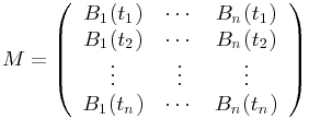
be the corresponding collocation matrix.

Schoenberg/Whitney [SW 53] proved that M is invertible if and only if for .

In fact, much more is true about the matrix M when . M is a TN matrix, as demonstrated by Karlin in [Kar68]. In [Boo76] it was verified that all minors of M are nonnegative and a particular minor is positive (when if and only if all main diagonal entries of that minor are positive. Such matrices are also known as almost totally positive matrices.

0.3 ORGANIZATION AND PARTICULARITIES

This book is divided into 11 chapters including this introductory chapter on TN matrices. The next chapter, Chapter 1, carefully spells out a number of basic and fundamental properties of TN matrices along with a compilation of facts and results from core matrix theory that are useful for further development of this topic. For our purposes, as stated earlier, a matrix will be considered over the real field, unless otherwise stated. Further, it may be the case that some of the results will continue to hold over more general fields, although they will only be stated for matrices over the reals.

Chapter 2 introduces and methodically develops the important and useful topic of bidiagonal factorization. In addition to a detailed description regarding the existence of such factorizations for TN matrices, we also discuss a number of natural consequences and explain the rather important associated combinatorial objects known as planar diagrams.

The next four chapters, Chapters 3–6, highlight the fundamental topics: recognition of TN matrices (Chapter 3); sign variation of vectors (Chapter 4); spectral properties (Chapter 5); and determinantal inequalities (Chapter 6).

The remaining four chapters cover a wide range of topics associated with TN matrices that are of both recent and historical interest. Chapter 7 contains a detailed account of the distribution of rank deficient submatrices within a TN matrix, including a discussion of the important notion of row and column inclusion. Chapter 8 introduces the Hadamard (or entrywise) product and offers a survey of the known results pertaining to Hadamard products of TN matrices, including a note on Hadamard powers. In Chapter 9, we explore the relatively modern idea of matrix completion problems for TN matrices. This chapter also includes a section on single entry perturbations, known as retractions, which turn out to be a useful tool for other problems on TN matrices. In Chapter 10 we conclude with a brief review of a number of subtopics connected with TN matrices, including powers and roots of TN matrices, TP/TN polynomial matrices, subdirect sums of TN matrices, and Perron complements of TN matrices.

For the reader we have included a brief introductory section with each chapter, along with a detailed account of the necessary terms and notation used within that chapter. We have aimed at developing, in detail, the theory of totally nonnegative matrices, and as such this book is sequential in nature. Hence some results rely on notions in earlier chapters, and are indicated accordingly by references or citations as necessary. On a few occasions some forward references have also been used (e.g., in section 2.6 a reference is made to a result to appear in Chapter 3). We have tried to keep such instances of forward references to a minimum for the benefit of the reader.

This work is largely self-contained with some minor exceptions (e.g., characterization of sign-regular transformations in Chapter 4). When a relevant proof has been omitted, a corresponding citation has been provided. In addition, some of the proofs have been extracted in some way from existing proofs in the literature, and in this case the corresponding citation accompanies the proof.

We have also included, at the end, a reasonably complete list of references on all facets of total nonnegativity. Finally, for the benefit of the reader, an index and glossary of symbols (nomenclature) have also been assembled.