Chapter Two

Bidiagonal Factorization

2.0 INTRODUCTION

Factorization of matrices is one of the most important topics in matrix theory, and plays a central role in many related applied areas such as numerical analysis and statistics. In fact, a typical (and useful) preliminary topic for any course in linear algebra is Gaussian elimination and elementary row operations, which essentially represents the groundwork for many forms of matrix factorization. In particular, triangular factorizations are a byproduct of many sorts of elimination strategies including Gaussian elimination.

Investigating when a class of matrices (such as positive definite or TP) admit a particular type of factorization is an important study, which historically has been fruitful. Often many intrinsic properties of a particular class of matrices can be deduced via certain factorization results. For example, it is a well-known fact that any (invertible) M-matrix can be factored into a product of a lower triangular (invertible) M-matrix and an upper triangular (invertible) M-matrix. This LU factorization result allows us to immediately conclude that the class of M-matrices is closed under Schur complementation, because of the connection between LU factorizations and Schur complements.

Matrix factorizations for the class of TN (TP) matrices have been well studied and continue to be a vital avenue for research pertaining to this class. Specifically, we are most interested in preserving the property of TN (or TP) for various factorization results. This constraint aids the focus for using these factorizations to exhibit properties of TN (or TP) matrices (cf. with the example above for M-matrices).

In this chapter our main focus will be on triangular factorization extended beyond just LU factorization. The most important factorization that will be studied here is the so-called “bidiagonal factorization.” A list of references for this topic is lengthy; see, for example, [And87, BFZ96, CP94B, CP97,Cry73,Cry76,FZ99,GP92,GP93B,GP94,GP96,Loe55,Pen97,RH72,Whi52] for further discussion on factorizations of TN matrices.

The basic observation that any TN matrix A can be written as A=LU, where L and U are lower and upper triangular TN matrices, respectively, was established in the nonsingular case in 1972 and later generalized to the singular case; see [Cry73] and [Cry76]. To obtain this stronger result, Cryer focused on unusual row and column operations not typically used in classical Gaussian elimination. Great care must be exercised in such an argument, as many row and column operations do not preserve total nonnegativity. Even though Whitney did not prove explicitly that any nonsingular TN matrix can be factored into lower and upper triangular TN matrices, she provided an observation that, in fact, implies more.

Suppose is an n-by-n matrix with , and for . Then, let B be the n-by-n matrix obtained from A by using row j to eliminate . Whitney essentially proved that A is TN if and only if B is TN. This observation serves as the foundation for a bidiagonal factorization result for TP matrices.

It is not clear why Whitney did not continue with this elimination scheme, as it would have led to a factorization of a nonsingular TN matrix into a product of TN bidiagonal matrices. In 1955 such a bidiagonal factorization result appeared for nonsingular TN matrices in [Loe55], where it was attributed to Whitney.

As far as we can discern, Theorem 2.2.2 was first stated in [Loe55], where it was used for an application to Lie-group theory. In [Loe55] the reference to a bidiagonal factorization of an invertible TN matrix was attributed to Whitney and her work in [Whi52], although Whitney did not make such a claim in her paper. More accurately, in [Whi52] a lemma was proved that is needed to establish the existence of such a factorization. More recently, such authors as Gasca, Peña, and others considered certain bidiagonal factorizations for which a specified order of row operations is required to ensure a special and appealing form for the factorization. They refer to this particular factorization as a Neville factorization or elimination (see [CP97,GP92,GP93B,GP94,GP96]). The work in [Cry76], and previously in [Cry73], seems to be the first time it is shown that a singular TN matrix also admits such a bidiagonal factorization. See [BFZ96] and the sequel [FZ99] for an excellent treatment of the combinatorial and algebraic aspects of bidiagonal factorization. Some of the graphical representations provided in [BFZ96] (and also [Bre95]) are employed throughout this book, and have been very useful for proving many results.

Other factorizations have also been considered for TN matrices; see, for example, [Cry76,GP94, Pen97,RH72]. The following factorization seems to be useful for various spectral problems for TN matrices (see also Chapter 5).

Theorem 2.0.1 If A is an n-by-n TN matrix, then there exist a TN matrix S and a tridiagonal TN matrix T such that

(i) TS=SA, and

(ii) the matrices A and T have the same eigenvalues.

Moreover, if A is nonsingular, then S is nonsingular.

This result was first proved in the nonsingular case in [RH72], and the general case was later proved by in [Cry76]. In Chapter 5 we will make use of a slightly modified version of this factorization to aid in characterizing properties about the positive eigenvalues of an irreducible TN matrix.

2.1 NOTATION AND TERMS

We begin this chapter by defining necessary terms and setting the required notation for understanding the topic of bidiagonal factorization.

Let I denote the n-by-n identity matrix, and for , we let E_ij denote the n-by-n standard basis matrix whose only nonzero entry is a 1 that occurs in the (i,j) position. An n-by-n matrix is called:

(1) diagonal if whenever ;

(2) tridiagonal if whenever ;

(3) upper (lower) triangular if whenever (i<j).

A tridiagonal matrix that is also upper (lower) triangular is called an upper (lower) bidiagonal matrix. Statements referring to just triangular or bidiagonal matrices without the adjectives “upper” or “lower” may be applied to either case.

It is necessary (for clarity of composition) to distinguish between two important classes of bidiagonal matrices. This will aid the development of the bidiagonal factorization over the next few sections.

Definition 2.1.1 (elementary bidiagonal matrices) For any positive integer n and complex numbers s,t, we let

for . Matrices of the form or above will be called elementary bidiagonal matrices, and the class of elementary bidiagonal matrices will be denoted by EB.

Definition 2.1.2 (generalized elementary bidiagonal matrices) Matrices of the form or , where n is a positive integer, s,t are complex numbers, and , will be called generalized elementary bidiagonal matrices, and this class will be denoted by GEB.

Since EB matrices are contained among the class of the so-called “elementary” matrices, EB matrices correspond to certain elementary row and column operations. For example, if A is an n-by-n matrix, then the product replaces row i of A by row i plus s times row i-1. Similarly, the product replaces column j by column j plus t times column j-1.

Also, because corresponds to an elementary row operation, it immediately follows that

Notice that all row/column operations using EB matrices only involve consecutive rows and columns.

Observe that any GEB matrix is TN whenever D is entrywise nonnegative and , and any EB matrix is (invertible) TN whenever .

In an effort to exhibit a factorization of a given matrix A into EB matrices, it is useful to consider the most natural elimination ordering when only considering EB matrices.

Recall that under typical “Gaussian elimination” to lower triangular form the (1,1) entry is used to eliminate all other entries in the first column (so-called pivoting), then moving to the 2nd column the (2,2) entry is used to eliminate all entries in column 2 below row 2, and so on. In this case we write the elimination (of entries) ordering as follows:

Using only EB matrices this elimination ordering is not appropriate for the simple reason that once the (2,1) entry has annihilated we cannot eliminate the (3,1) entry with EB matrices. This is different, however, from claiming that a matrix of the form

has no (lower) EB factorization. In fact,

The key item here is that we first had to multiply A by (on the left), which essentially filled in the (2,1) entry of A, that is,

Now we use the (2,1) entry of to eliminate the (3,1) entry, and so-on.

Consider another useful example. Let

We begin by using the second row to eliminate the (3,1) entry of V and continue eliminating up the first column to obtain

Then we shift to the second column and again use the second row to eliminate the (3,2) entry, yielding

or . Applying similar row operations to the transpose U^T, we can write U as , where .

Hence, we can write the (Vandermonde) matrix V as

(2.1)

In general, a better elimination ordering strategy is to begin at the bottom of column 1 and eliminate upward, then repeat this with column 2, and so on. In this case the elimination (of entries) ordering is given by

which (in general) will reduce A to upper triangular form, say U. The same elimination ordering can be applied to U^T to reduce A to diagonal form. This elimination scheme has also been called “Neville elimination”; see, for example, [GP96].

For example, when n=4, the complete elimination order is given by

which is equivalent to (bidiagonal) factorization of the form:

(2.2)

This particular ordering of the factors has been called a successive elementary bidiagonal factorization and a Neville factorization.

For brevity, we may choose to shorten the factorization in (2.2) by just referring to the subscripts that appear in each of the Ls and Us in (2.2). For example, to represent (2.2) we use

As in [JOD99], we refer to the product of the factors within ( ) (like (234)) as a stretch.

Recall that an n-by-n matrix A is said to have an LU factorization if A can be written as A=LU, where L is an n-by-n lower triangular matrix and U is an n-by-n upper triangular matrix.

2.2 STANDARD ELEMENTARY BIDIAGONAL FACTORIZATION: INVERTIBLE CASE

Consider a 3-by-3 Vandermonde matrix V given by

(2.3)

Expressing a matrix as a product of a lower triangular matrix L and an upper triangular matrix U is called an LU-factorization. Such a factorization is typically obtained by reducing a matrix to upper triangular form via row operations, that is, by Gaussian elimination. If all the leading principal minors of a matrix are nonzero, then Gaussian elimination can always proceed without encountering any zero pivots; see [HJ85, p. 160]. For example, we can write V in (2.3) as

(2.4)

Such a factorization is unique if L is lower triangular with unit main diagonal, and U is upper triangular.

We use the elementary matrices to reduce L to a diagonal matrix with positive diagonal entries. As was shown in the previous section, . Applying similar row operations to the transpose U^T, we can write U as , where .

Hence, we can write the (Vandermonde) matrix V as

(2.5)

We are leading to the main result that any InTN matrix has a bidiagonal factorization into InTN bidiagonal factors.

There are two very important impediments to proving that such a factorization exists via row operations using only EB matrices:

(1) to ensure that the property of being TN is preserved, and

(2) to avoid accidental cancellation.

Before we discuss these issues we should keep in mind that if A is invertible, then the reduced matrix obtained after a sequence of row operations is still invertible.

Item (1) was answered in the pioneering paper [Whi52], where she actually worked out the very crux of the existence of a bidiagonal factorization for InTN matrices, which is cited in [Loe55]. We now discuss in complete detail A. Whitney’s key result and demonstrate its connections to the bidiagonal factorization of InTN matrices.

Theorem 2.2.1 (Whitney’s key reduction result) Suppose has the property that , and for all . Then A is TN if and only if is TN.

Proof. Let . Then any minor of B that does not involve row j+1 is certainly nonnegative, since A is TN. In addition, any minor of B that includes both row j and row j+1 is nonnegative since it is equal to the corresponding minor of A by properties of the determinant. Thus let

be any minor of B with and . Then by the properties of the determinant it follows that

To show that , it is enough to verify the following equivalent determinantal inequality:

(2.6)

To prove this inequality, first let us consider the case that . Then let

(2.7)

In this case C is an (t+1)-by-(t+1) TN matrix, and the inequality (2.6) is equivalent to proving that

(2.8)

To prove (2.8) we will instead prove a more general determinantal inequality for TN matrices, which can also be found in [GK02, p. 270].

Claim: Let be an n-by-n TN matrix. For each i,j, let . Then for and we have

(2.9)

Proof of claim: Note it is enough to assume that the rank of A is at least n-1; otherwise all terms in (2.9) are zero. Now observe that (2.9) is equivalent to

(2.10)

for . Moreover, (2.10) is equivalent to

(2.11)

where A_s is obtained from A by replacing the entries by 0. When n=2, inequality (2.11) is obvious. Assume that (2.11) is valid for such matrices of order less than n.

Suppose that for some with and , we have . If no such minor exists, then observe that to compute each A_i1 we could expand along column 1 of A_i1 (or column 2 of A), in which case each A_i1 would be zero, and again all terms in (2.9) are zero.

Hence assume that , where ; otherwise we could compute A_i1 () by expanding along row x<s. Now permute the rows of A_s such that row x is first and row y is last, and call the new matrix . Then by Sylvester’s determinantal identity applied to we have

Taking into account the effect to the determinant by column switches, the above equality is the same as

By induction both (x<s) and (s<y) are nonnegative. Hence , which completes the proof of the claim.

Now if , define C to be as above with the first column repeated; then the inequality (2.6) is equivalent to (2.8) for this new matrix C.

Finally, using (2.10) for the matrix C as in (2.7), and for s=j, we have

since , for . Clearly the above inequality is exactly the inequality (2.6). This completes the proof.

Observe that there is a similar Whitney reduction result that can be applied to the first row of A by considing the transpose.

Using Whitney’s reduction fact, it follows that an invertible TN matrix can be reduced to upper triangular form by applying consecutive row operations starting from the bottom of the leftmost column and working up that column, then shifting columns. This reduction to upper triangular form depends on the fact that there is no accidental cancellation along the way (see item (2) above). Because A. Whitney was the first (as far as we can tell) to prove that the property of TN is preserved under this row operation scheme, we will refer to this elimination scheme as the Whitney elimination, instead of, say, the Neville elimination as used by others (see, for example, [GP96]).

The next important topic to address is (item (2) above) how to avoid accidental cancellation when applying the Whitney elimination to an InTN matrix. The answer follows from the simple observation that if is InTN, then . This fact is easily verified, since if for some i, then by the double echelon form of any TN matrix (notice A cannot have any zero lines), A would have a block of zeros of size i-by-n-i+1 (or n-i+1-by-i), which implies that A is singular, as the dimensions of the zero block add to n+1. Since is InTN (Theorem 2.2.1) whenever A is InTN, we could never encounter the situation in which and (assuming we are eliminating in the jth column). The reason is that in this case the kth row of this matrix would have to be zero, otherwise this matrix will have some negative 2-by-2 minor, and, in particular, would not be in double echelon form. Thus any InTN matrix can be reduced to upper triangular from (while preserving the property of InTN) via TN EB matrices; such a factorization using the Whitney elimination scheme will be called an successive elementary bidiagonal factorization (denoted by SEB). We now state in full detail the complete SEB factorization result for InTN matrices.

Theorem 2.2.2 Any n-by-n invertible TN matrix can be written as

(2.12)

where ; for all ; and is a diagonal matrix with all .

Proof. The proof is by induction on n. The cases n=1,2 are trivial. Assume the result is true for all InTN matrices of order less than n. Suppose A is an n-by-n InTN matrix. Then applying Whitney’s reduction lemma to the first column of A and the first row of A, we can rewrite A as

Here α >0 and A’ is InTN. Now apply induction to A’. To exhibit the factorization in (2.12) simply direct sum each TN EB matrix with the matrix [1] and the diagonal factor with α. This completes the proof.

For example, a 4-by-4 InTN matrix A can be written as

(2.13)

Theorem 2.2.2 grew out of the work in [Whi52], which contains a key preliminary reduction result involving certain row operations on TP matrices. This result appeared explicitly in [GP96] in connection with the so-called Neville elimination. It actually appeared first (without proof) in [Loe55], where it was referred to as Whitney’s theorem. In any event, Theorem 2.2.2 is and continues to be an important and useful characterization of TP matrices; see also [FZ00].

Part of the attraction of the SEB factorization is the natural connection to the Whitney elimination ordering. The multipliers that arise in each EB matrix can be expressed in terms of certain ratios of products of minors of the original matrix, which lead to important and useful determinantal test criterion (see Chapter 3, Section 1) for verifying if a given matrix is TP or InTN.

Specifically, for TP matrices it follows that no multiplier could ever be zero, since all minors are positive. Moreover, the converse holds, which we state as a corollary to Theorem 2.2.2.

Corollary 2.2.3 An n-by-n matrix is TP if and only if it can be written as

(2.14)

where ; for all ; and is a diagonal matrix with all .

Example 2.2.4 [symmetric Pascal matrix] Consider the special case of the factorization (2.13) of a 4-by-4 matrix in which all the variables are equal to one. A computation reveals that the product (2.13) is then the matrix

(2.15)

which is necessarily TP.

On the other hand, consider the n-by-n matrix whose first row and column entries are all ones, and for let . The matrix P_n is called the symmetric Pascal matrix because of its connection with Pascal’s triangle. When n=4,

Thus, P₄ is the matrix A in (2.15), so P₄ is TP. In fact, the relation implies that P_n can be written as

Hence, by induction, P_n has the factorization (2.12) in which the variables involved are all equal to one. Consequently, the symmetric Pascal matrix P_n is TP for all .

Note that in the above factorization each elementary bidiagonal matrix is in fact TN. If a matrix admits such a factorization, we say that A has a successive bidiagonal factorization and denote this by SEB.

The final important topic to discuss is the issue of uniqueness of the SEB factorization for TP and InTN matrices.

In general, the first part of an SEB factorization (reduction only to upper triangular form) that follows from the Whitney elimination ordering (or scheme) can be abbreviated to

To prove the uniqueness of this factorization (assuming this order of the TN EB matrices), assume two such factorizations exist for a fixed TP or InTN matrix A. Starting from the left, suppose the first occurrence of a difference in a multiplier occurs in the jth factor in the product . Then cancel from the left all common EB matrices until we arrive at the EB matrix corresponding to the jth factor in . So then the simplified factorization can be written as

Suppose the multipliers in the EB matrices in the leftmost product above are denoted by (in order) . By construction we are assuming that the multiplier is different.

First observe that j>k, since for this simplified factorization the (k,k-1) entry of A is uniquely determined by the factorization and is equal to . Furthermore, the entries in positions of A are easily computed in terms of the multipliers above. In particular, for the entry in position (t,k-1) of A is equal to . Since the entry in position (k,k-1) is uniquely determined and is equal to , it follows, assuming that all multipliers involved are positive, that all subsequent multipliers (or EB factors) are the same in both factorizations by working backward from the entries in positions (k,k-1) to (j,k-1). Hence the multiplier must be the same in both factorizations, which is a contradiction.

In the event that some multiplier, say for some , then observe that for all . Otherwise (recalling item (2) above regarding no accidental cancellation) we must have encountered a zero row at some point in the reduction process, which contradicts the fact that A was invertible. Hence the multiplier in both factorizations, again a contradiction.

A nice consequence of the existence of an SEB factorization for any n-by-n InTN matrices is that an InTN matrix can be written as a product of n-1 InTN tridiagonal matrices. This fact requires a short argument regarding the relations that exist for the matrix algebra generated by such EB matrices.

2.3 STANDARD ELEMENTARY BIDIAGONAL FACTORIZATION: GENERAL CASE

For singular TN matrices it is natural to ask if there are corresponding bidiagonal factorization results as in the case of InTN or TP. As a matter of fact, such results do exist although depending on the preponderance of singular submatrices or the rank deficiency, obtaining such a factorization can be problematic. However, in 1975 C. Cryer established in complete detail the existence of a bidiagonal factorization for any (singular) TN matrix into generalized TN EB matrices. Of course depending on the nature of the singularity, the bidiagonal factors may themselves be singular, so as a result we should longer expect in general that:

(1) the factorization to be unique,

(2) the factors to be EB matrices, or

(3) all the “singularity” to be absorbed into the middle diagonal factor.

Consider the following illustrative example.

Let

Then observe that A is a singular TN matrix. Moreover, notice that A can be factored into bidiagonal TN factors in the following two ways:

and

The difficulties that arise when considering (1)–(3) above were all taken into account by Cryer when he proved his factorization result for TN matrices. In fact, Cryer was more interested in exhibiting a bidiagonal factorization than in determining the possible number, or order of the associated TN factors. It should be noted that Cryer did pay attention to the types of bidiagonal factors used to produce such a factorization, and in particular verified that the factors were generalized TN EB matrices. Also he was well aware that such a factorization was not unique.

As pointed out in the 1976 paper [Cry76] there are two major impediments when attempting to produce a bidiagonal factorization of a singular TN matrix:

(1) we may encounter a zero row, or

(2) we may encounter a “degenerate” column (i.e., a zero entry occurs above a nonzero entry).

Both (1) and (2) above could come about because of accidental cancellation. Consider the following examples:

Notice that in the second case we have no way of eliminating the (3,2) entry.

Much of the analysis laid out in [Cry76] was to handle these situations. Before we give arguments to circumvent these difficulties, it is worth taking a moment to inspect the zero/nonzero pattern to determine the exact nature of the degeneracies that may occur. For example, if during the elimination process we observe that in column a nonzero entry ends up immediately below a zero entry, then every entry in the row to the right of the zero must also be zero. Moreover, if there is a nonzero entry in column i above the identified zero entry in row k, then the entire kth row must be zero. Finally, if all entries above the nonzero in column i are zero, then there must be a zero in every position (s,t) with and , namely in the upper right block formed by rows and column .

Assume when it comes time to eliminate in column that we are in the following scenario:

(1) we have been able to perform the desired elimination scheme up to column i, and

(2) , , for t>k; for ; and .

Under these assumptions, we know that rows must all be zero, in which case we (in a manner of speaking) can ignore these rows when devising a matrix to apply the required row operation. Let denote the m-by-m matrix given by . To “eliminate” the (k,i) entry, observe that this matrix, call it A, can be factored as A=LA, where , where the matrix occupies rows and columns . It is easy to check that A’ has a zero in the (k,i) position, and still possesses the desired triangular form. Moreover, it is clear that L is TN, as is TN whenever .

However, the matrix is not a bidiagonal matrix! This situation can be easily repaired by noting that, for example,

It is straightforward to determine that can be factored in a similar manner. Thus can be factored into TN generalized EB matrices.

The final vital observation that must be verified is that the resulting (reduced) matrix is still TN. This follows rather easily since zero rows do not affect membership in TN; so, ignoring rows , the property of preserving TN is a consequence of Whitney’s original reduction result (see Theorem 2.2.1).

Upon a more careful inspection of this case, we do need to consider separately the case j<i, since we are only reducing to upper triangular form. In this instance (as before) we note that rows are all zero, and the procedure here will be to move row k to row i. In essence we will interchange row k with row i via a bidiagonal TN matrix, which is possible only because all rows in between are zero. For example, rows k and k-1 can be interchanged by writing A as A=GA, where A’ is obtained from A by interchanging rows k and k-1, and where G is the (singular) bidiagonal TN matrix given by , with

Note that the matrix G₂ in the matrix G is meant to occupy rows and columns k-1,k. The point here is to avoid non-TN matrices (such as the usual transposition permutation matrix used to switch rows), and to derive explicitly the factorization into a product of TN matrices. This is vital since both A and G are singular.

Finally, if we go back to A and notice that all entries in column i above a_ki are all zero, then we can apply similar reasoning as in the previous case and move row k to row i, and then proceed.

Up to this point we have enough background to state, and in fact prove, the result on the bidiagonal factorization of general TN matrices ([Cry76]).

Theorem 2.3.1 [Cry76] Any n-by-n TN matrix A can be written as

(2.16)

where the matrices L⁽ⁱ⁾ and U^(j) are, respectively, lower and upper bidiagonal TN matrices with at most one nonzero entry off the main diagonal.

The factors L⁽ⁱ⁾ and U^(j) in (2.16) are not required to be invertible, nor are they assumed to have constant main diagonal entries, as they are generalized EB matrices.

We intend to take Theorem 2.3.1 one step farther and actually prove that every TN matrix actually has an SEB factorization, where now the bidiagonal factors are allowed to be singular. Taking into account the possible row/column interchanges and the fact that possibly non-bidiagonal matrices are used to perform the elimination (which are later factored themselves as was demonstrated earlier), there is a certain amount of bookkeeping required to guarantee that such a factorization exists. To facilitate the proof in general will use induction on the order of the matrix.

To begin consider (separately) the case n=2. Let

be an arbitrary 2-by-2 TN matrix. If a>0, then

and thus A has an SEB factorization into bidiagonal TN matrices.

On the other hand, if a=0, then at least one of b or c is also zero. Suppose without loss of generality (otherwise consider A^T) that b=0. Then in this case,

and again A has an SEB factorization into bidiagonal TN matrices.

Recall that matrices of the form or , where n is a positive integer, s,t are real numbers, and , are called GEB matrices. To avoid any confusion with EB matrices from the previous section we devise new notation for generalized bidiagonal matrices. For any , we let denote the elementary lower bidiagonal matrix whose entries are

We are now in a position to state and prove that any TN matrix has an SEB factorization into generalized bidiagonal matrices of the form .

Theorem 2.3.2 Any n-by-n TN matrix can be written as

(2.17)

where ; for all ; and is a diagonal matrix with all .

Proof. Suppose first that the (1,1) entry of A is positive. We begin eliminating up the first column as governed by the Whitney ordering until we encounter the first instance of a zero entry (in the first column) immediately above a nonzero entry. If this situation does not arise, then we continue eliminating up the first column.

Suppose and . Assume that the first positive entry in column 1 above row k is in row j with , such a j exists since . Then as before all rows between the jth and kth must be zero. To ‘eliminate’ the (k,1) entry observe that A can be factored as A=LA, where , where the matrix occupies rows and columns .

Moreover, we observed that the matrix L can be factored as

which is the correct successive order of generalized bidiagonal matrices needed to perform the Whitney ordering from rows k to j.

Now assume that the (1,1) entry of A is zero. In this case the only remaining situation that could arise is if all of column 1 above row k is zero and . Then rows are zero. Then we can interchange row k with row 1 by factoring A as

by using the matrix G₂ in the appropriate positions. Again this is the correct successive order to go from rows k to 1 in the Whitney ordering.

After having completed the elimination procedure on column 1, we proceed by eliminating row 1 in a similar successive manner to achieve

where and B is TN. By induction B has an SEB factorization into generalized bidiagonal matrices.

If α=0, then direct sum each generalized bidiagonal factor in an SEB factorization of B with a 1-by-1 zero matrix to obtain an SEB factorization of A. Notice that in this case both row and column 1 of A must have been zero. If α >0, then direct sum each generalized bidiagonal factor in an SEB factorization of B with a 1-by-1 matrix whose entry is a one except for the diagonal factor, which is to be adjoined (by direct summation) with a 1-by-1 matrix whose entry is α. In each case we then obtain an SEB factorization of A, as desired.

Thinking more about the EB matrices L_i and U_j there are in fact relations satisfied by these matrices that are important and, for example, have been incorporated into the work in [BFZ96]. Some of these relations are:

(1) , if ;

(2) , for all i;

(3) , for each i and where for we have that ; and

(4) , if .

Naturally, relations (1)–(3) also exist for the upper EB matrices U_j. Relations (1)–(3) are simple computations to exhibit. Relation (4) is also straightforward when , but if i=j, then a rescaling by a positive diagonal factor is required. Hence, in this case we have a relation involving GEB matrices. For example, , and if , then .

As a passing note, we acknowledge that there have been advances on bidiagonal factorizations of rectangular TN matrices, but we do not consider this topic here. For those interested, consult [GT06, GT06b, GT08].

2.4 LU FACTORIZATION: A CONSEQUENCE

It is worth commenting that the SEB factorization results discussed in the previous sections are extensions of LU factorization. However, it may be more useful or at least sufficient to simply consider LU factorizations rather than SEB factorizations.

The following remarkable result is, in some sense, one of the most important and useful results in the study of TN matrices. This result first appeared in [Cry73] (although the reduction process proved in [Whi52] is a necessary first step to an LU factorization result) for nonsingular TN matrices and later was proved in [Cry76] for general TN matrices; see also [And87] for another proof of this fact.

Theorem 2.4.1 Let A be an n-by-n matrix. Then A is (invertible) TN if and only if A has an LU factorization such that both L and U are n-by-n (invertible) TN matrices.

Using Theorem 2.4.1 and the Cauchy-Binet identity we have the following consequence for TP matrices.

Corollary 2.4.2 Let A be an n-by-n matrix. Then A is TP if and only if A has an LU factorization such that both L and U are n-by-n ΔTP matrices.

Proof. Since all the leading principal minors of A are positive, A has an LU factorization; the main diagonal entries of L may be taken to be 1, and the main diagonal entries of U must then be positive. Observe that

The fact that if follows by applying similar arguments to the minor . To conclude that both L and U are ΔTP we appeal to Proposition 3.1.2 in Chapter 3.

That any TN matrix can be factored as a product of TN matrices L and U is, indeed, important, but for the following application (see also the section on subdirect sums in Chapter 10) we need rather more than what is contained in Theorem 2.4.1. When the TN matrix A has the form

we need that, in addition to being lower and upper triangular, respectively, the (correspondingly partitioned) L has its 3,1 block and U its 1,3 block equal to zero. In case A₁₁ is invertible, a simple partitioned calculation reveals that this must occur in any LU factorization of A (since L₁₁ and U₁₁ will be invertible). However, when A₁₁ is singular, there can occur TN matrices A of our form that have TN LU factorizations with positive entries in the L₃₁ or U₁₃ blocks. Fortunately, though, LU factorizations will be highly nonunique in this case, and there will always exist ones of the desired form. Thus, an auxiliary assumption that A₁₁ is invertible would avoid the need for Lemma 2.4.3, but this somewhat specialized lemma (perhaps of independent interest, though it requires an elaborate proof) shows that such an auxiliary assumption is unnecessary.

Let

and let , , denote the r-by-r matrix

Observe that both of the above matrices are TN.

Lemma 2.4.3 Let

in which A₁₁, A₂₂, and A₃₃ are square. Suppose A is TN. Then

in which L and U (partitioned conformally with A) are both TN.

Proof. The proof is by induction on the size of A. The case n=2 is trivial. For completeness, however, we handle the case n=3 separately. Suppose A is a 3-by-3 matrix of the form

There are two cases to consider. Suppose . Then A can be written as

Now we can apply induction to the bottom right block of the matrix in the middle. On the other hand if , then we can assume that , in which case A can be written as

Again we can apply induction to the bottom right block of the second factor above. The general case is handled similarly.

If the (1,1) entry of A is positive, then no row or column switches are needed to reduce A to

Here we allow the possibility of some of the generalized EB matrices to be equal to I, and note that A’ will have the same form as A. Hence induction applies.

On the other hand if the (1,1) entry of A is zero, then we may assume without loss of generality that the entire first row of A is zero. If column 1 of A is zero, then apply induction. Otherwise suppose that is the first positive entry in column 1. Then A can be reduced without row interchanges to

Now we can apply the matrix F₂, as used in the case n=3, to reduce A’ to

Now induction can be applied to the matrix A. In either case we obtain the desired LU factorization. This completes the proof.

2.5 APPLICATIONS

As indicated by the lengthy discussion, SEB factorizations of TN matrices are not only important in their own right, but they also arise in numerous applications (see [GM96]).

Perhaps the most natural application is simply generating matrices in this class. As noted earlier constructing TP or TN matrices directly from the definition is not only difficult but extremely tedious. The number of conditions implied by ensuring all minors are positive are too numerous to check by hand. However, armed with the SEB factorizations for TN and TP matrices (see Theorem 2.3.2 and Corollary 2.2.3), to generate TN or TP matrices, it suffices to choose the parameters that arise in these factorizations nonnegative or positive, respectively. By this we mean that if all multipliers in an SEB factorization are chosen to be positive along with the diagonal factor, then the resulting product is guaranteed to be TP; while if all multipliers in (2.17) are chosen to be nonnegative, then the resulting product is TN.

Similarly, if the diagonal factor is chosen to be positive in (2.12) and all the multipliers are nonnegative, then the resulting product will be InTN. A subtle issue along these lines is when we can be sure that such an InTN matrix, constructed as above, is actually oscillatory?

In fact the answer is known and will be described completely in the next section. It was shown in [GK02, p. 100] that an InTN matrix A is oscillatory if and only if for each i.

Another less obvious (but not difficult) application of SEB factorizations is the classical fact (see [GK02, Kar65, Whi52, And87]) that the topological closure of the TP matrices is the TN matrices. We are only concerned with Euclidean topology in this case. Most proofs of this fact require some clever fiddling with the entries of the matrix (often via multiplication with a certain TP matrix– the Polya matrix). Again using only the SEB factorization, the proof of this closure result is immediate. For any TN matrix, write a corresponding SEB factorization into generalized TN EB matrices. Then perturb each such generalized EB matrix by making the multiplier positive (and small), and by making the diagonal entries of each factor positive and small. After this we can pass a positive diagonal factor through the Ls and Us to ensure that each generalized EB matrix is actually an EB TN matrix. By Corollary 2.2.3, the resulting product must be TP. Moreover, this product can be chosen to be as “close” to A as we wish.

A less useful but straightforward implication is that if A is InTN, then is InTN. This result follows trivially from the SEB factorization because , so that , which is a TN EB matrix. The same argument applies to the EB matrices U_j, and observe that is a positive diagonal matrix. Hence it follows that is InTN.

Another application we present in this section deals with a specific issue from one-parameter semigroups. In [Loe55] the bidiagonal factorization (2.12) of TN matrices was used to show that for each nonsingular n-by-n TN matrix A there is a piecewise continuous family of matrices Ω (t) of a special form such that the unique solution of the initial value problem

(2.18)

has A(1)=A.

Loewner was interested in the theory of one-parameter semigroups. Along these lines, let be a differentiable matrix-valued function of t such that A(t) is nonsingular and TN for all , and . From this

(2.19)

is often referred to as an infinitesimal element of the semigroup of nonsingular TN matrices.

Loewner observed that an n-by-n matrix is an infinitesimal element if and only if

(2.20)

He then showed that the nonsingular TN matrices obtained from a constant satisfying (2.20) with only one nonzero entry are either (a) diagonal matrices with positive main diagonal entries or (b) the elementary bidiagonal matrices or in which . From here he applied Theorem 2.2.2 to show that every nonsingular TN matrix can be obtained from the solution of the initial value problem (2.18).

Recall the symmetric Pascal matrix P_n in Example 2.2.4. Consider the solution A(t) of (2.18) in which , the creation or derivation matrix, given by the lower bidiagonal TN matrix

Then is a polynomial of degree n-1 in Ht, and the Pascal matrix , necessarily TN and nonsingular, has entries

The symmetric Pascal matrix is , so it is also TN; see [AT01] for more details.

The final application we present here deals with computer-aided geometric design and corner cutting algorithms. Over the past years, there has been a considerable amount of research conducted on developing algorithms in computer-aided geometric design (CAGD) that may be classified as corner cutting algorithms. An example of such algorithms makes use of evaluating a polynomial curve using the Bernstein basis. It is known (see [MP99]) that the Bernstein basis is a basis for the space of all polynomials of degree at most n with optimal shape preserving properties, which is due, in part, to the variation diminishing property of TN matrices (see also Chapter 4). It turns out that bidiagonal matrices and bidiagonal factorization have an important connection to corner cutting algorithms. Following the description in [MP99], an elementary corner cutting may be viewed as a mapping of a polygon with vertices into another polygon with vertices defined by: for some , () and for ; or for some , () and for . Such corner cuttings may be defined in terms of GEB TN matrices, and since a corner cutting algorithm is a composition of elementary corner cuttings, such algorithms may be described by a product of corresponding GEB TN matrices, and hence this product is TN. The reader is urged to consult [MP99] and other related references where corner cutting algorithms are described.

2.6 PLANAR DIAGRAMS AND EB FACTORIZATION

As discussed earlier, TN matrices arise in many areas of mathematics. Perhaps one of the most notable interplays comes from TP matrices and combinatorics. This connection, which will be discussed in more detail shortly, seems to be explicit (in some form) in [Bre95], although some of his analysis builds on existing fundamental results, such as Lindstrom’s work on acyclic weighted directed graphs to compute determinants.

We now discuss the connection between SEB factorizations and planar diagrams or networks by introducing the associated diagrams, stating and verifying Lindström’s lemma, and then using it to demonstrate how to calculate minors of the corresponding matrix. We also direct the reader to the important work of on transition matrices associated with birth and death processes (see [KM59]).

Roughly speaking we associate a simple weighted digraph to each EB matrix and diagonal factor. Then from this we will obtain a larger weighted directed graph corresponding to an SEB factorization by concatenation of each smaller diagram.

An excellent treatment of the combinatorial and algebraic aspects of bidiagonal factorization of TN matrices along with generalizations for totally positive elements in reductive Lie groups is given in [BFZ96,FZ99,FZ00]. One of the central tools used in these papers and others is a graphical representation of the bidiagonal factorization in terms of planar diagrams (or networks) that can be described as follows.

An n-by-n diagonal matrix is represented by the elementary diagram on the left in Figure 2.1, while an elementary lower (upper) bidiagonal matrix () is the diagram middle (right) of Figure 2.1.

Figure 2.1 Elementary diagrams

Each horizontal edge of the last two diagrams has a weight of 1. It is not difficult to verify that if A is a matrix represented by any one of the diagrams in the figure, then is nonzero if and only if in the corresponding diagram there is a family of t vertex-disjoint paths joining the vertices on the left side of the diagram with the vertices on the right side. Moreover, in this case this family of paths is unique, and is equal to the product of all the weights assigned to the edges that form this family. Given a planar network and a path connecting a source and a sink, the weight of this path is defined to be the product of the weights of its edges, and the weight of a collection of directed paths is the product of their weights.

To extend this notion further, we consider the case n=3 for clarity of exposition. The general case is a straightforward extension of this case and is omitted here. Interested readers may consult [FZ99, Bre95, BFZ96, FZ00] and other references.

One of the benefits of considering these weighted planar networks or planar diagrams (or acyclic directed graphs) is the connection to computing minors of the matrices associated with a given planar network. To this end, consider the product of two 3-by-3 EB matrices

Recall the Cauchy-Binet determinantal identity

As observed above, is obtained by calculating the (sum of the) weights of all collections of vertex disjoint paths from rows (source set) α to columns (sink set) γ. Similarly, is obtained by calculating the (sum of the) weights of all collections of vertex disjoint paths from rows (source set) γ to columns (sink set) β. Thus as γ runs through all k subsets of (here ), each such summand (or product) constitutes the weight of a collection of vertex disjoint paths from source set α to an intermediate set γ, and then to sink set β. Such a collection of paths can be realized as a collection of vertex disjoint paths in the diagram obtained by concatenating the diagrams (in order) associated with and (see Figure 2.2). In other words, is equal to the sum of the weights of all families of vertex-disjoint paths joining the vertices α on the left of the concatenated diagram with the vertices β on the right.

Figure 2.2 Concatenation of elementary diagrams

This analysis can be extended to an arbitrary finite product of EB matrices in the following manner. Given a product in which each matrix A_i is either a diagonal matrix or an (upper or lower) EB matrix, a corresponding diagram is obtained by concatenation left to right of the diagrams associated with the matrices . Then the Cauchy-Binet formula for determinants applied to the matrix A implies the next two results (which are sometimes called Lindstrom’s lemma).

Proposition 2.6.1 Suppose in which each matrix A_i is either a diagonal matrix or an (upper or lower) EB matrix. Then:

(1) Each (i,j)-entry of A is equal to the sum over all paths joining the vertex i on the left side of the obtained diagram with the vertex j on the right side of products of all the weights along the path.

(2) is equal to the sum over all families of vertex-disjoint paths joining the vertices on the left of the diagram with the vertices on the right of products of all the weights assigned to edges that form each family.

For example, in an arbitrary SEB factorization of a 3-by-3 InTN matrix given by

the associated planar network is constructed as shown in Figure 2.3.

In particular, the factorization in (2.1) can be written as

and the planar network corresponding to this factorization of V is presented in Figure 2.4.

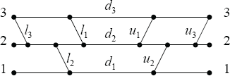
Figure 2.3 General 3-by-3 planar network

Figure 2.4 Planar network corresponding to the factorization (2.1)

The edges in Figure 2.4 are all oriented left to right. This network contains 3 sources at the left and 3 sinks at the right. Each slanted edge corresponds to the positive entry off the main diagonal of one TN EB matrix in the factorization (2.1). The order of these edges coincides with the order of the factors in (2.1). All horizontal edges have weight one except, possibly, the horizontal edges in the middle of Figure 2.4 that correspond to the main diagonal entries of D.

Theorems 2.2.2 and 2.3.2 imply that every TN matrix can be represented by a weighted planar diagram constructed from building blocks as in Figure 2.1 (in the case of degenerate matrices some of the horizontal edges may have to be erased).

A minor extension along these lines is to associate TN matrices with more general weighted planar digraphs (see [Bre95]). One defines a planar diagram of order n as a planar acyclic digraph with all edges oriented from left to right and 2n distinguished boundary vertices: n sources on the left and n sinks on the right with both sources and sinks labeled from bottom to top. To each edge of a planar diagram we assign a positive weight, and we denote by W the collection of all weights of the edges. We refer to the pair as a weighted planar diagram of order n. Clearly, the diagrams in Figure 2.1 and concatenations thereof are weighted planar diagrams of order n.

Suppose is a given weighted planar diagram of order n. Then we may apply the first statement in Proposition 2.6.1 as a definition of an n-by-n matrix associated with . It was first observed in [KM59] that the second statement remains valid in this more general situation and, in particular, is TN.

A wonderfully useful byproduct to considering planar networks associated to TN, InTN, or TP matrices is that, in this setting, every minor of such a matrix is a subtraction-free polynomial in the parameters associated with the EB matrices that make up the SEB factorization. For example, if A is represented by the planar network in Figure 2.3, then

This consequence is extremely important and particularly useful for studying determinantal inequalities among minors of TN matrices (see also Chapter 6).

For example, consider Fischer’s determinantal inequality, which can be stated as follows. Let be TN and let be any index set. Then

where α^c denotes the complement of α relative to .

The proof of Fischer’s inequality given in [GK02, p. 131] relies on Sylvester’s determinantal identity and the fact that the TP matrices are dense in the set of TN matrices. Here is a proof that uses the bidiagonal factorization for TP matrices.

Fix an index set α, and factor A as in (2.17). By the Cauchy-Binet identity and the fact that each elementary bidiagonal matrix has ones on the main diagonal we have

which completes the proof.

Hadamard’s inequality for TN can be derived from Fischer’s inequality as follows. Fischer’s inequality ensures that for any TN matrix . Now apply induction to the TN submatrix .

Before we move on to further results, we first present a proof of the fact that if all the multipliers are positive in the SEB factorization (2.14), then the resulting product is totally positive. Notice that it is sufficient to prove that if all the multipliers l_i are positive, then the resulting product is a lower triangular ΔTP matrix. When n=2, this result is immediate. So assume it is true for all such lower triangular matrices of order less than n. Suppose L is a lower triangular matrix obtained from multiplying all the lower TN EB matrices in (2.14) in which all the multipliers are positive. Let Γ be the corresponding planar diagram for L. To prove that L is ΔTP, it is enough to exhibit the existence of a collection of vertex-disjoint paths from source set to sink set with the property that for in Γ. Since all possible slanted edges are present, it follows from induction (here we only consider the section Γ after the stretch and ignoring the bottom level associated to the vertex 1) that there exists a collection of vertex-disjoint paths from α to β whenever . Thus there are two cases remaining: (i) (and hence ); or (ii) and . In case (i) the only path from vertex 1 to vertex 1 is along the bottom of Γ, so combining this unique path with the collection of vertex disjoint paths from to , which is guaranteed by induction, we have the existence of a collection of vertex-disjoint paths from α to β. In case (ii) send i₁ to one via the shortest possible path using the first slanted edges possible, and send to by first passing by the stretch corresponding to and then applying induction. As before, this implies existence of a collection of vertex-disjoint paths from α to β. Hence for all such to sink set with the property that for in Γ. Therefore L is ΔTP.

A common theme in this book is to interchange the notions of SEB factorizations and planar diagrams when dealing with various properties of TN matrices. In particular, we will often think of a TN matrix by merely representing it as a general planar network (as in Figure 2.3 for n=3). Given such a correspondence, we can recast Theorems 2.2.2 and 2.3.2 and Corollary 2.2.3 in terms of planar networks.

Theorem 2.6.2 If Γ is a planar network corresponding to (2.12), then:

(1) The associated matrix is InTN if and only if all the weights of the EB parameters are nonnegative and all .

(2) The associated matrix is TP if and only if all the weights of the EB parameters are positive and all .

Theorem 2.6.3 If Γ is a planar network corresponding to (2.17), then the associated matrix is TN if and only if all the weights of the generalized EB parameters are nonnegative (including the main diagonal of each factor) and all .

We close this section with a short subsection illustrating the connections between SEB factorizations and oscillatory matrices which were eluded to in Section 2.5.

2.6.1 EB Factorization and Oscillatory Matrices

It is evident from a historical perspective that oscillatory matrices (or IITN matrices) play a key role both in the development of the theory of TN matrices, and also in their related applications (see [GK02], for example). Incorporating the combinatorial viewpoint from the previous section, we recast some of the classical properties of oscillatory matrices. We begin with a characterization (including a proof) of IITN matrices described entirely by the SEB factorization (see [Fal01]).

Theorem 2.6.4 Suppose A is an InTN matrix with corresponding SEB factorization given by (2.12). Then A is oscillatory if and only if at least one of the multipliers from each of and each of is positive.

Proof. Suppose all the multipliers from some L_k are zero. Then there is no path from k to k-1 in the planar network associated with (2.12). Hence the entry in position k,k-1 of A must be zero, which implies A is not oscillatory.

For the converse, suppose that for every L_i, U_j there is at least one positive multiplier (or parameter). Then since A is invertible all horizontal edges of all factors are present, and hence there exists a path from k to both k-1 and k+1 for each k (except in extreme cases where we ignore one of the paths). In other words, whenever . Thus it follows that A is oscillatory.

In their original contribution to this subject, Gantmacher and Krein did establish a simple yet informative criterion for determining when a TN matrix was oscillatory, which we state now.

Theorem 2.6.5 [GK] (Criterion for being oscillatory) An n-by-n TN matrix is oscillatory if and only if

As presented in [GK02] their proof makes use of some minor technical results. For example, they needed to define a new type of submatrix referred to as quasi-principal to facilitate their analysis. It should be noted that part of the purpose of examining quasi-principal submatrices was to verify the additional claim that if A is an n-by-n oscillatory matrix, then necessarily is totally positive. Again the fact that the (n-1)st power is shown to be a so-called critical exponent was also hinted by tridiagonal TN matrices, as the (n-1)st power of an n-by-n tridiagonal matrix is the first possible power in which the matrix has no zero entries.

The next observation may be viewed as a combinatorial characterization of IITN matrices, at least in the context of an SEB factorization, may be found in [Fal01].

Theorem 2.6.6. Suppose A is an n-by-n invertible TN matrix. Then is TP if and only if at least one of multipliers from each of and each of is positive.

We omit the details of the proof (see [Fal01]), but the general idea was to employ the method of induction, incorporate SEB factorizations, and apply the important fact that if A is TN, then A is TP if and only if all corner minors of A are positive (for more details see Chapter 3).

As in the original proof by Gantmacher and Krein we also established that if A is oscillatory, then necessarily is TP. Furthermore, all the n-by-n oscillatory matrices for which the (n-1)st power is TP and no smaller power is TP have been completely characterized by incorporating the powerful combinatorics associated with the planar diagrams (see [FL07]).

Another nice fact that is a consequence of the results above states when a principal submatrix of an IITN matrix is necessarily IITN. The same fact also appears in [GK60] (see also [GK02, p. 97]).

Corollary 2.6.7 Suppose A is an n-by-n IITN matrix. Then A[α] is also IITN, whenever α is a contiguous subset of N.

As an aside, a similar result has appeared in [FFM03] but, given the general noncommutative setting, the proof is vastly different.

The next result connects Theorem 2.6.6 to the classical criterion of Gantmacher and Krein for oscillatory matrices (Theorem 2.6.5); see also [Fal01].

Theorem 2.6.8 Suppose A is an n-by-n invertible TN matrix. Then and , for if and only if at least one of multipliers from each of and each of is positive.

It is apparent that factorization of TN matrices are an extremely important and increasingly useful tool for studying oscillatory matrices. Based on the analysis in [FFM03], another subset of oscillatory matrices was defined and called basic oscillatory matrices. As it turns out, basic oscillatory matrices may be viewed as minimal oscillatory matrices in the sense of the fewest number of bidiagonal factors involved.

In [FM04] a factorization of oscillatory matrices into a product of two invertible TN matrices that enclose a basic oscillatory matrix was established. A different proof of this factorization was presented by utilizing bidiagonal factorizations of invertible TN matrices and certain associated weighted planar diagrams in [FL07b], which we state now.

Suppose A is an oscillatory matrix. Then A is called a basic oscillatory matrix if A has exactly one parameter from each of the bidiagonal factors and is positive. For example, an IITN tridiagonal matrix is a basic oscillatory matrix, and, in some sense, represents the main motivation for considering such a class of oscillatory matrices.

Theorem 2.6.9 Every oscillatory matrix A can be written in the form A= S B T, where B is a basic oscillatory matrix and S, T are invertible TN matrices.