Chapter Six

Determinantal Inequalities for TN Matrices

6.0 INTRODUCTION

In this chapter we begin an investigation into the possible relationships among the principal minors of TN matrices. A natural and important goal is to examine all the inequalities among the principal minors of TN matrices. More generally, we also study families of determinantal inequalities that hold for all TN matrices.

In 1893, Hadamard noted the fundamental determinantal inequality

(6.1)

holds whenever A=[a_ij] is a positive semidefinite Hermitian matrix. Hadamard observed that it is not difficult to determine that (6.1) is equivalent to the inequality

(6.2)

where A=[a_ij] is an arbitrary n-by-n matrix.

In 1908, Fischer extended Hadamard’s inequality (6.1) by demonstrating that

(6.3)

holds for any positive semidefinite Hermitian matrix A and for any index set . Recall that A[S] denotes the principal submatrix of A lying in rows and columns S, and for brevity we will let S^c denote the complement of S relative to N (that is, ). As usual we adopt the convention that . Evidently, Hadamard’s inequality (6.1) follows from repeated application of Fischer’s inequality by beginning with . For a detailed survey on various principal minor inequalities of the standard positivity classes the reader is directed to the paper [FJ00].

Around the time of World War II, Koteljanskii was interested in many aspects of positivity in linear algebra, and, among his many interesting and important contributions was a unifying theory of a certain class of determinantal inequalities involving principal minors, which now bear his name. Formally, Koteljanskii generalized Fischer’s inequality (6.3) within the class of positive semidefinite matrices, and, perhaps more importantly, he extended the class of matrices (beyond positive semidefinite) for which this inequality is valid (see [Kot53, Kot63]). As Koteljanskii inequalities play a fundamental role in the field of determinantal inequalities, we expend some effort to carefully explain this seminal result.

For an n-by-n matrix A, and any two index sets , Koteljanskii’s inequality states:

(6.4)

It is apparent, for any positive semidefinite matrix, that Koteljanskii’s inequality implies Fischer’s inequality (bearing in mind the convention ), and hence is a generalization of both Fischer’s and Hadamard’s inequalities.

In addition, Koteljanskii observed that (6.4) holds for a larger class of matrices, which includes the positive semidefinite matrices. Before we can derive this class, we should recall some key definitions.

Recall that a matrix is called a P₀-matrix if all its principal minors are nonnegative. Consider the subclass of P₀-matrices A that satisfy

(6.5)

for any two index sets with the properties:

(1) and

(2) .

We note that a minor of the form , where U and V satisfy the conditions and , has been called an almost principal minor (in the sense that the index sets U,V differ only in precisely one index). Note that condition (6.5) requires that all symmetrically placed almost principal minors have the same sign (ignoring zeros), and it is obvious that not all P₀-matrices satisfy (6.5). It is clear that any positive semidefinite matrix satisfies (6.5), and it is also clear that any TN also satisfies (6.5). A slightly more general result is that (6.5) holds for both M-matrices and inverse M-matrices as well (see, for example, [Car67, FJ00]) for more details.

Perhaps an even more useful property is that if A is an invertible P₀-matrix and satisfies (6.5), then is P₀ and satisfies (6.5), see [FJ00].

The main observation [Kot53, Kot63] is the following fact.

Theorem 6.0.1 Suppose A is an n-by-n P₀-matrix. Then A satisfies (6.4) for all index sets U,V satisfying (1) and (2) above if and only if A satisfies (6.5) for all index sets S,T.

For simplicity of notation, if A is a P₀-matrix that satisfies (6.4) for all index sets S,T, then we call A a Koteljanskii matrix, and denote the class of all Koteljanskii matrices by .

The punch line is then that both TN matrices and positive semidefinite (as well as M and inverse M) matrices satisfy Koteljanskii’s determinantal inequality, and therefore they also satisfy both Fischer’s inequality and Hadamard’s inequality. Moreover, all these determinantal inequalities lie naturally within a general family of multiplicative minor inequalities which we survey further throughout the remainder of this chapter. In fact, the study of determinantal inequalities has seen a reemergence in modern research among linear algebraists (see, for example [BJ84] and subsequent works [FJ00, FJ01, FGJ03]), where an important theme emerged; namely, to describe all possible inequalities that exist among products of principal minors via certain types of set-theoretic conditions. Employing this completely combinatorial notion led to a description of the necessary and sufficient conditions for all such inequalities on three or fewer indices, and also verified other inequalities for cases of more indices, all with respect to positive semidefinite matrices.

Our intention here is to employ these ideas and similar ones more pertinent to theory of TN matrices to derive a similar description. One notable difference between the class of TN matrices and the positive semidefinite matrices is that TN matrices are not in general closed under simultaneous permutation of rows and columns, while positive semidefinite matrices are closed under such an operation.

6.1 DEFINITIONS AND NOTATION

Recall from Chapter 0 that for a given n-by-n matrix, and , A[S,T] denotes the submatrix of A lying in rows S and columns T. For brevity, A[S,S] will be shortened to A[S].

More generally, if is a collection of index sets (i.e., ), and , we let

denote the product of the principal minors , . For example, if for any two index sets S, T, then

If, further, is another collection of index sets with , then we write with respect to a fixed class of matrices if

for each . Thus, for instance, if and for any two index sets S, T, then the statement with respect to the class is a part of Koteljanskii’s theorem (Theorem 6.0.1).

We shall also find it convenient to consider ratios of products of principal minors. For two such collections α and β of index sets, we interpret as both a numerical ratio for a given matrix, and also as a formal ratio to be manipulated according to natural rules. When interpreted numerically, we obviously need to assume that for A, and we note that if A is InTN, then , for all index sets S. Consequently, when discussing ratios of products of principal minors, we restrict ourselves to InTN (or even TP) matrices.

Since, by convention, , we also assume, without loss of generality, that in any ratio both collections α and β have the same number of index sets, since if there is a disparity between the total number of index sets in α and β, the one with fewer sets may be padded out with copies of π. Also, note that either α or β may include repeated index sets (which count).

When considering ratios of principal minors, we may also be interested in determining all pairs of collections α and β such that

(6.6)

for some constant K (which may depend on n), and for all A in InTN. We may also write , with respect to InTN.

As a matter of exposition, if given two collections α and β of index sets, and with respect to TN, then we have determined a (determinantal) inequality, and we say the ratio is bounded by 1. For example, if and for any two index sets S, T, then the ratio is bounded by 1 with respect to InTN (and invertible matrices in ). If, further, with respect to InTN, then we say is bounded by the constant K with respect to InTN.

6.2 SYLVESTER IMPLIES KOTELJANSKII

As suggested in the previous section, the work of Koteljanskii on determinantal inequalities and the class of matrices is so significant in the area of determinantal inequalities that we continue to study this topic, but from a different angle. In this section, we demonstrate how Sylvester’s determinantal identity can be used to verify Koteljanskii’s theorem (Theorem 6.0.1). In some sense, Sylvester’s identity is implicitly used in Koteljanskii’s original work, so this implication is not a surprise, but nonetheless it is still worth discussing.

Recall that a special instance of Sylvester’s identity (1.5) is

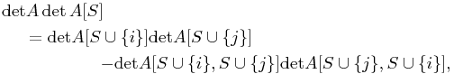
where , with and . Thus for any matrix in , we can immediately deduce that

as for all such S (cf. (6.5). Observe that the inequality

is an example of a Koteljanskii inequality. In fact, it is a very special example of such an inequality, and we refer to it as a basic Koteljanskii inequality. To be more precise, a Koteljanskii inequality is called basic if it is of the form,

in which , and . In this case, it is evident that . Such conditions are intimately connected with the almost principal minors that were discussed in the previous section. From the above analysis, it is clear that Sylvester’s identity can be used to verify basic Koteljanskii inequalities for all matrices in .

To make the exposition simpler, we define a notion of “gap.” For two index sets , we define the gap of S and T as

Observe that for all , gap, and if gap or 1, then the corresponding Koteljanskii inequality is trivial. Summarizing parts of the discussion above essentially establishes that if gap, then Koteljanskii’s holds for sets S and T assuming that A was in . However, we outline the argument in the gap two case for completeness.

Proposition 6.2.1 Suppose S and T are two index sets such that gap. Then

for any A satisfying (6.5).

Proof. If gap for two index sets S and T, then one of the following cases must hold: (1) , or (2) . If case (2) occurs, then the corresponding Koteljanskii inequality is trivial, and, if (1) holds, then , and the corresponding Koteljanskii inequality is basic, and thus valid.

The idea for the proof of the main result is to reduce the gap by one and apply induction, using Proposition 6.2.1 as a base case. We state the next result in terms of ratios, so we are implicitly assuming the use of invertible matrices. The general case then follows from continuity considerations. For brevity, we may let (S) denote .

Proposition 6.2.2 Suppose S and T are two index sets for which the associated Koteljanskii inequality holds and gap. Then for any invertible A satisfying (6.5) we have

such that

Proof. Without loss of generality, assume that . Since gap (implying a nonbasic inequality), we know that , and hence there must exist an index , so that . Consider the set-theoretic factorization

Observe that both factors represent (in a natural way) Koteljanskii ratios and that the gap for each factor on the right is less than gap(s,t), by construction. Applying a simple induction argument will complete the proof.

Proposition 6.2.2 gives rise to two interesting consequences, both of which are useful to note and follow below. The other item we wish to bring attention to is the proof technique used for establishing Proposition 6.2.2: namely, connecting the verification of a numerical ratios by extending this notion to a factorization (or product) of ratios of index sets. This idea will appear often in the next few sections.

Corollary 6.2.3 For matrices in , basic Koteljanskii inequalities may be viewed (set-theoretically) as a generating set for all Koteljanskii inequalities. That is, any valid Koteljanskii inequality may be rewritten as a product of basic Koteljanskii inequalities.

Corollary 6.2.4 Let A be an n-by-n matrix satisfying (6.5). Then Sylvester’s determinantal identity can be used to verify that Koteljanskii’s inequality

holds for all pairs of index sets S,T.

6.3 MULTIPLICATIVE PRINCIPAL MINOR INEQUALITIES

One of the central problems in this area is to characterize, via set-theoretic conditions, all pairs of collection of index sets such that

over all InTN matrices A. It is clear that since TP is the closure of TN (and hence of InTN), that the bounded ratios with respect to InTN and with respect to TP are the same.

This general issue was resolved in [FHJ98] for the case of M-matrices and inverse M-matrices. In fact, the bound K can always be chosen to be one for both the M- and the inverse M-matrices. The same problem has received much attention for positive semidefinite matrices (see, for example, [BJ84]), but a general resolution in this case seems far off.

We now turn our attention to the case of InTN matrices, and we begin with an illustrative example, that in many ways was the impetus of the investigation that began in [FGJ03].

Example 6.3.1 Let and . Then , for any InTN matrix A, which can be seen by

On the other hand, if and , then is not a valid inequality in general, since if

then and , where is arbitrary.

These basic examples illustrate two particular points regarding determinantal inequalities for TN/TP matrices. First, arbitrary permutation of the indices in the collections α and β of an established bounded ratio need not produce a bounded ratio, and, second, verification of a bounded ratio can be intricate and subtle.

Let be any collection of index sets from N. For , we define to be the number of index sets in α that contain the element i. In other words, counts the number of occurrences of the index i among the index sets in α.

The following proposition, which represents a basic necessary condition, demonstrates that in order for any ratio to be bounded with respect to the TN/TP matrices, the multiplicity of each index in α and β must coincide (see [FGJ03]).

Proposition 6.3.2 Let α and β be two collections of index sets. If is bounded with respect to the class of TN matrices, then , for every .

Proof. Suppose there exists an index i for which . For let , where the number k occurs in the th entry of . Then is an invertible TN matrix for every such value of k. Evaluation of at gives

Hence is unbounded, since we may select or as according to the sign of .

If is a given ratio that satisfies the condition , for every , then we say that satisfies condition set-theoretic zero, ST0 for short. It is clear that ST0 is not a sufficient condition for a ratio to be bounded with respect to InTN; see the previous example. Furthermore, since the closure of the TP matrices is the TN matrices, ST0 is also a basic necessary condition for any ratio to be bounded with respect to TP.

The fact that any TN (InTN, TP) matrix has an elementary bidiagonal factorization proves to be very useful for verifying the boundedness of a given ratio.

Suppose we are presented with a specific ratio . To verify that this ratio is unbounded, say with respect to InTN, we need to show that there exists choices for the nonnegative parameters and and choices for the positive parameters , such that increases without bound faster than β(A), when A is written as in (2.12).

Now an important item to keep in mind is that when A is presented via its elementary bidiagonal factorization, then both α(A) and β(A) are subtraction-free (polynomial) expressions in the nonnegative variables and and the positive variables . Along these lines, if we are able to identify a subcollection of these variables for which the degree with respect to this subcollection in α(A) exceeds the corresponding degree in β(A), then we may assign all the variables in this subcollection the single variable , and set all remaining variables be equal to 1. Under this assignment, both α(A) and β(A) are polynomials in the single variable t with . Thus, letting implies that is not a bounded ratio. Consider the following ratio (written set-theoretically):

Let A be an arbitrary InTN matrix, and suppose A is written in terms of its SEB factorization:

Then, it is easily verified that

and

If, for example, we set , and all remaining variables to one, then α(A) is a polynomial in t of degree 4, whereas β(A) is a polynomial in t of degree 3. Consequently, increases without bound as , and therefore is an unbounded ratio with respect InTN.

On the other hand, the ratio

is, indeed, a bounded ratio with respect to InTN. To see this, observe that the difference (which is a subtraction-free expression)

for all nonnegative values of the parameters (here we are assuming A is presented as above). Hence with respect to InTN.

A more general necessary condition for a proposed ratio to be bounded is known, and makes use of a notion of majorization (see [FGJ03]).

Given two nondecreasing sequences of nonnegative integers such that , we say that M₁ majorizes M₂ (denoted ) if the following inequalities hold:

Conjugate sequences are defined by

(6.7)

It is well known that if and only if .

Now let be two collections of index sets. Let be any contiguous subset of N. We call such an index set L an interval. Define to be a sequence of numbers rearranged in a nondecreasing order.

Given a ratio , we say that this ratio satisfies condition (M) if

(6.8)

see also [FGJ03] with proof.

Figure 6.1 A general n-by-n diagram

Theorem 6.3.3 If the ratio is bounded, then it satisfies condition (M).

Proof. First, note that the condition follows from Proposition 6.3.2. Next, let L=N. For , consider a TP matrix that corresponds to the diagram in Figure 6.1 with weights equal to t and the rest of the weights equal to 1. Then, for any , the degree of as a polynomial in t is equal to . It follows that , where is a sequence conjugate to defined as in (6.7). Thus conditions necessary for to be bounded translate into inequalities . Therefore, or, equivalently, . Now, to prove (6.8) for an arbitrary interval , it is sufficient to apply the above argument to InTN matrices of the form for .

Corollary 6.3.4 For , let (resp. ) denote the number of index sets in α (resp. β) that contain J. If the ratio is bounded, then for every interval .

Proof. It suffices to notice that all elements of are not greater than and exactly of them are equal to .

Remark. In [BJ84], it is shown that a ratio is bounded with respect to the class of positive definite matrices, if , for every subset (the converse need not hold). In [FHJ98], part of one of the main results can be stated as follows: a ratio is bounded with respect to the class of M-matrices if and only if it satisfies: , for all , and , for every subset . We note here that the condition for arbitrary J is neither necessary nor sufficient (see [Fal99]) for a ratio to be bounded with respect to the InTN matrices.

6.3.1 Characterization of Principal Minor Inequalities for

A collection of bounded ratios with respect to InTN is referred to a generator if and only if any bounded ratio with respect to InTN can be written as products of positive powers of ratios from this collection. The idea employed is to assign the weights , in which t is a nonnegative variable that we make arbitrarily large, to the variables . For such a weighting, each principal minor will then be a function in terms of t. For a ratio of principal minors to be bounded, the degree of t in the denominator must be greater than or equal to the degree of t in the numerator. As before, we may let (S) denote .

We consider the 3-by-3 case in full detail, which can also be found in [FGJ03]. Every ratio on 3 indices can be written in the following way:

where is the degree of in the ratio. Let be the degree of t in . Then the expression

represents the degree of t in this ratio. By assumption, we set . Then, , and the simplified expression has the form For this ratio to be bounded, Using diagrams with different weightings, we produce a list of conditions, each of the form Condition ST0 (for n=3) is equivalent to and

Example 6.3.5 Let A be a 3-by-3 invertible TN matrix,

For the matrix A, a simple computation yields , , , and . Thus , , , and . Therefore, the expression represents the total degree of t in any ratio. In order for a ratio to be bounded with respect to InTN, it must satisfy the condition

In the 3-by-3 case, consider the following four necessary conditions (see Figure 6.2) that are used to define the cone of bounded ratios. Because the edges of the left side of each diagram are all weighted 1, it is sufficient to consider the right side only (see [FGJ03]).

Figure 6.2 Necessary diagrams for 3-by-3 case

Each of the graphs in Figure 6.2 gives rise to a halfspace

This list of inequalities can be written as a matrix inequality , in which A is a 4-by-4 real matrix and we can define an associated polyhedral cone In the 3-by-3 case we then have the following characterization of all bounded ratios (see [FGJ03] for a complete proof).

Theorem 6.3.6 Suppose is a ratio of principal minors on three indices. Then is bounded with respect to the invertible TN matrices if and only if can be written as a product of positive powers of the bounded ratios

Proof. The four diagrams in Figure 6.2 give rise to the following four necessary conditions: (a) ; (b) ; (c) ; and (d) . Recall that the necessary conditions (ST0) are equivalent to the three equations and For simplicity of the analysis we use the equations above to convert the four inequalities to “greater than” inequalities, namely, (a) ; (b) ; (c) ; and (d) . Fix . Then the intersection given by the linear inequalities: , , and , forms a polyhedral cone. Translate the variables to so that the corresponding inequalities, in terms of z, are translated to the origin. Observe that the intersection of is the ray given by ; the remaining extreme rays are determined similarly. In this case, the polyhedral cone C formed by the intersection of the above hyperplanes is given by . Therefore any vector may be written as . Writing these equations in terms of x gives , , and . Using the equations given by (ST0), we may now solve for the remaining variables, for example, . Similarly, it follows that , and . Finally, we substitute the above x-values back into the original ratio, that is,

where . This completes the proof.

For the cases n=4 and 5, the analysis is similar but not surprisingly more involved. The number of necessary conditions increase, the number of variables increase, and the number of generators (or extremals) increases (see [FGG] and [FGJ03]). We summarize the main results from these works below.

Theorem 6.3.7 Suppose a ratio of principal minors on four indices. Then is bounded with respect to the invertible TN matrices if and only if can be written as a product of positive powers of the following bounded ratios:

Theorem 6.3.8 Suppose a ratio of principal minors on five indices. Then is bounded with respect to the invertible TN matrices if and only if can be written as a product of positive powers of the following bounded ratios:

Note that the generators in the list (38 in total) all consist of two sets over two sets just as in the n=3 and n=4 cases.

Since, by Corollary 6.3.14 (to follow), each of the ratios in Theorems 6.3.6, 6.3.7, and 6.3.8 is bounded by one, we obtain the following.

Corollary 6.3.9 For , any ratio of principal minors is bounded with respect to the invertible TN matrices if and only if it is bounded by one.

The above essentially represents the current state, in terms of complete characterizations of all of the principal minor inequalities with respect to InTN. It is clear that this technique could extend, however, the computation becomes prohibitive. One of the important properties of determinantal inequalities for InTN seems to be the underlying connection with subtraction-free expression (in this case with respect to the parameters from the SEB factorization).

6.3.2 Two-over-Two Ratio Result: Principal Case

As seen in the previous characterizations, ratios consisting of two index sets over two index sets seem to play a fundamental role. In fact, for , all the generators for the bounded ratios of products of principal minors have this form. Also, Koteljanskii’s inequality can be interpreted as a ratio of two sets over two sets.

Before our main observations of this section, we first consider the following very interesting and somewhat unexpected ratio (see [FGJ03]). We include a proof for completeness and to highlight the concept of subtraction-free expressions and their connections to determinantal inequalities for InTN.

Proposition 6.3.10 For any 4-by-4 invertible TN matrix the following inequality holds,

Proof. Consider an arbitrary 4-by-4 InTN matrix presented via its elementary bidiagonal factorization. Then it is straightforward to calculate each of the four 2-by-2 minors above. For instance, , , , and finally .

Next we compute the difference between the expressions for the denominator and the numerator, namely, . Observe that the above expression is a subtraction free expression in nonnegative variables and hence is nonnegative. This completes the proof.

We now move on to the central result of this section; consult [FGJ03] for complete details of the facts that follow.

Theorem 6.3.11 Let and be subsets of . Then the ratio is bounded with respect to the invertible TN matrices if and only if:

(1) this ratio satisfies (ST0); and

(2) for every interval .

The proof is divided into several steps. First, observe that the necessity of the conditions follows immediately from Theorem 6.3.2. Indeed, it is not hard to see that these conditions are equivalent to condition (M) for with .

Suppose γ is a subset of and L is a given interval of . Then we let . Finally, suppose that and are indices of , so that . Then we say the sequence interlaces the sequence if one of following cases occur: (1) and ; (2) l=k and ; or (3) and . In the event with and with (), and the sequence interlaces the sequence , then we say that γ interlaces δ. The next proposition follows immediately from the definitions above.

Proposition 6.3.12 Let γ and δ be two nonempty index sets of . If δ interlaces , then for every interval L.

We have already established the following inequalities with respect to the TN matrices: (Koteljanskii), , and (Proposition 6.3.10). These inequalities will serve as the base cases for the next result, which uses induction on the number of indices involved in a ratio (see [FGJ03]).

Theorem 6.3.13 Let γ and δ be two nonempty index sets of N. Then the ratio is bounded with respect to the invertible TN matrices if and only if for every interval L of N.

Observe that Theorem 6.3.13 establishes that main result in this special case of the index sets having no indices in common.

Proof of Theorem 6.3.11: Note that the ratio is bounded with respect to the invertible TN matrices if and only if is bounded with respect to the invertible totally nonnegative matrices, for some S and T obtained from and , respectively, by deleting common indices and shifting (as these operations preserve boundedness, see [FGJ03]).

There are many very useful consequences to Theorems 6.3.11 and 6.3.13, which we include here.

The proof of the above result follows directly from Theorem 6.3.13 and the fact that the base case ratios are each bounded by one; see [FGJ03] for more details.

Corollary 6.3.14 Let and . Then the ratio is bounded with respect to the invertible TN matrices if and only if it is bounded by one.

For the next consequence we let (i.e., the minor consisting of all the odd integers of N) and (the minor consisting of all the even integers of N). Then the next result follows directly from Theorem 6.3.13.

Corollary 6.3.15 For , and ,

for any TN matrix. Of course the first inequality is just Fischer’s inequality.

6.3.3 Inequalities Restricted to Certain Subclasses of InTN/TP

As part of an ongoing effort to learn more about all possible principal minor inequalities over all TN/TP matrices, it is natural to restrict attention to important subclasses. Along these lines two subclasses have received some significant attention: the tridiagonal InTN matrices and a class known as STEP 1.

Suppose A is a tridiagonal InTN matrix; then A is similar (via a signature matrix) to an M-matrix. As a result, we may apply the characterization that is known for all multiplicative principal minor inequalities with regard to M-matrices. In doing so, we have the following characterization (see [FJ01]). We begin with the following definition, and note that the condition presented has a connection to condition (M) restricted to ratios consisting of two index sets.

Let be a given collection of index sets. We let denote the number of index sets in α that contain L, where . We say the ratio ratio satisfies (ST1)’ if

(6.9)

holds for all contiguous subsets L of N. This condition, in a more general form (namely, the condition holds for all subsets of N), has appeared in the context of determinantal inequalities for both positive semidefinite and M-matrices (see [BJ84, FHJ98] and the survey paper [FJ00]).

Now, for tridiagonal matrices, the next property is key for the characterization that follows. If A is a tridiagonal matrix, then

where ⊕ denotes direct sum. In particular,

It is clear that to compute a principal minor of a tridiagonal matrix it is enough to compute principal minors based on associated contiguous index sets.

The main result regarding the multiplicative principal minor inequalities for tridiagonal matrices (see [FJ01]) is then

Theorem 6.3.16 Let be a given ratio of index sets. Then the following are equivalent:

(i) satisfies (ST0) and (ST1)’;

(ii) is bounded with respect to the tridiagonal TN matrices;

(iii) with respect to the tridiagonal TN matrices.

We also bring to the attention of the reader that there is a nice connection between the determinantal inequalities that hold with respect to the tridiagonal TN matrices and Koteljanskii’s inequality (see [FJ01]).

Another subclass that has been studied in this context has been referred to as the class STEP 1. As a consequence of the SEB factorization of any InTN matrix, we know that other orders of elimination are possible when factoring an InTN matrix into elementary bidiagonal factors. For instance, any InTN matrix A can be written as

where for all ; and D is a positive diagonal matrix. Further, given the factorization above (6.10), we introduce the following notation:

Then (6.10) is equivalent to

The subclass of interest is defined as follows. The subclass STEP 1 is then defined as . The name is chosen because of the restriction to one (namely, the first) stretch of elementary bidiagonal (lower and upper) factors in the factorization (6.10).

For this class, all the multiplicative principal-minor inequalities have been completely characterized in terms of a description of the generators for all such bounded ratios. As with the general case, all ratios are bounded by one and all may be deduced as a result of subtraction-free expressions for the difference between the denominator and numerator (see [FL08]). All generators are of the form

where and we adopt the convention that if , then we drop j+1 from the ratio above, or if , then we drop i-1 from the ratio above.

6.4 SOME NON-PRINCIPAL MINOR INEQUALITIES

Certainly the possible principal minor inequalities that exist among all TN/TP matrices are important and deserve considerably more attention. However, TN/TP matrices enjoy much more structure among their non-principal minors as well, and understanding the inequalities among all (principal and non-principal) minors throughout the TN/TP matrices is of great value and interest. In fact, as more analysis is completed on general determinantal inequalities, it is becoming more apparent (see, for example, [BF08, FJ00, FL08, Ska04]) that this analysis implies many new and interesting inequalities among principal minors.

We extend some of the notation developed earlier regarding minors to include non-principal minors. Recall that for an n-by-n matrix A and , the submatrix of A lying in rows indexed by and columns indexed by is denoted by . For brevity, we may also let denote . More generally, let denote a collection of multisets (repeats allowed) of the form , where for each i, denotes a row index set and denotes a column index set (, ). If, further, is another collection of such index sets with for , then, as in the principal case, we define the concepts such as

and , the ratio (assuming the denominator is not zero), bounded ratios and generators with respect to InTN.

6.4.1 Non-Principal Minor Inequalities: Multiplicative Case

Consider the following illustrative example. Recall that

with respect to InTN. Moreover, this ratio was identified as a generator for all bounded ratios with respect to 3-by-3 InTN matrices, and hence cannot be factored further into bounded ratios consist of principal minors.

On the other hand, consider the ratio of non-principal minors

It is straightforward to verify that this ratio is bounded by 1 with respect to TP (this ratio involves a 2-by-3 TP matrix only), and is actually a factor in the factorization

Since each factor on the right is bounded by one, the ratio on the left is then also bounded by one.

Thus, as in the principal case, a similar multiplicative structure exists for bounded ratios of arbitrary minors of TP matrices (we consider TP to avoid zero minors). And like the principal case (cf. Section 6.3.1), characterizing all the bounded ratios via a complete description of the (multiplicative) generators is a substantial problem, which is still rather unresolved. However, for , all such generators have been determined (see [FN]). In fact, the work in [FN] may be viewed as an extension of the analysis begun in [FGJ03].

The main observation from [FN] is the following result describing all the generators for all bounded ratios with respect to TP for .

Theorem 6.4.1 Suppose is a ratio of minors on three indices. Then is bounded with respect to the totally positive matrices if and only if can be written as a product of positive powers of the following bounded ratios:

Moreover, all the ratios above were shown to be bounded by one, so we may conclude that all such bounded ratios are necessarily bounded by one.

In an effort to extend Theorem 6.3.11 to general minors, one insight is to connect a minor of a TP matrix A with a corresponding Plücker coordinate. Recall from Chapter 1: The Plücker coordinate

where , is defined to be the minor of B(A) lying in rows and columns . That is,

Suppose α, β are two index sets of N of the same size and γ is defined as

where is the complement of β relative to N. Then for any n-by-n matrix A, we have

For simplicity, we will shorten to just . Then, we may consider ratios of Plücker coordinates with respect to TP such as

where (see [BF08]).

In [BF08] two ratios were identified and played a central role in the analysis that was developed within that work. The first type of ratio was called elementary and has the form

where , , and are not in Δ. It is evident that elementary ratios are connected with the short Plücker relation discussed in Chapter 1. The second key ratio type was referred to as basic and can be written as

with , , and are not in Δ. It was shown in [BF08] that every bounded elementary ratio is a product of basic ratios and (see below) that the basic ratios are the generators for all bounded ratios consisting of two index sets over two index sets. We also note that both basic and elementary ratios were also studied in [Liu08].

Theorem 6.4.2 Let be a ratio where are subsets of . Then the following statements are equivalent:

(1) satisfies STO and for every interval ;

(2) can be written as a product of basic ratios;

(3) is bounded by one with respect to TP.

We note here that some of the techniques used in the proof of Theorem 6.4.2 extend similar ones used in [FGJ03] to general minors of TP matrices. Furthermore, the equivalence of statements (1) and (3) was first proved in [Ska04]. In addition, in [RS06], the notion of multiplicative determinantal inequalities for TP matrices has been related to certain types of positivity conditions satisfied by specific types of polynomials.

As in the principal case, narrowing focus to specific subclasses is often beneficial, and some research along these lines has taken place. The two classes of note, which were already defined relative to principal minor inequalities, are the tridiagonal InTN matrices and STEP 1. For both of these classes all multiplicative minor inequalities have been characterized via a complete description of the generators. For STEP 1, all generators have the form:

where (see [FL08]). Observe the similarity between the form of the generators above and the basic ratios defined previously. For more information on the tridiagonal case, consult [Liu08].

6.4.2 Non-Principal Minor Inequalities: Additive Case

Since all minors in question are nonnegative, studying additive relations among the minors of a TN matrix is a natural line of research. Although the multiplicative case has received more attention than the additive situation, there have been a number of significant advances in the additive case that have suggested more study.

For example, in Chapter 2 we needed an additive determinantal inequality to aid in establishing the original elimination result by Anne Whitney. Recall that for any n-by-n TN matrix A=[a_ij] and for and for , we have

where, for each i,j, .

Another instance of a valid and important additive determinantal inequality is one that results from the Plücker relations discussed in Chapter 1, as each constructed coordinate is positive.

As a final example, we discuss the notion of a compressed matrix and a resulting determinantal inequality that, at its root, is an additive minor inequality for TN matrices. Consider nk-by-nk partitioned matrices , in which each block A_ij is n-by-n. It is known that if A is a Hermitian positive definite matrix, then the k-by-k compressed matrix (or compression of A)

is also positive definite, and

Comparing and identifying common properties between positive definite matrices and totally positive matrices is both important and useful, and so we ask: if A is a totally positive nk-by-nk matrix, then is the compressed matrix a totally positive matrix?

We address this question now by beginning with informative and interesting k=2 case, including a proof from [FGHJ06].

Theorem 6.4.3 Let A be a 2n-by-2n totally positive matrix that is partitioned as follows:

where each A_ij is an n-by-n block. Then the compression is also totally positive. Moreover, in this case

Proof. Since A is totally positive, A can be written as A=LU, where L and U are ΔTP matrices. We can partition L and U into n-by-n blocks and rewrite A=LU as

Observe that

Applying the classical Cauchy-Binet identity to the far right term above yields

where the sum is taken over all ordered subsets γ of with cardinality n. If we separate the terms with and , then the sum on the right in (6.11) reduces to

Since L and U are ΔTP, all summands are positive. Hence

which is equivalent to

Thus we have

and so , which completes the proof.

The following is a consequence of Theorem 6.4.3 and the classical fact that the TP matrices are dense in the TN matrices.

Corollary 6.4.4 Let A be a 2n-by-2n TN matrix that is partitioned as follows:

where A_ij is n-by-n. Then is also TN and

To extend this result for larger values of k, it seemed necessary to identify the determinant of the compressed matrix as a generalized matrix function (for more details see [FGHJ06]). In fact, it was shown that the compression of a -by- TP matrix is again TP, while for , compressions of nk-by-nk TP matrices need not necessarily be TP. Furthermore, in [FGHJ06] there are many related results on compressions of TP matrices.