
7
Transverse Wave Propagation in Bounded Media
Javier Brum
Laboratorio deAcustica Ultrasonora, Instituto de Fisica, Facultad de Ciencias, Universidad de la Republica, Montevideo, Uruguay
7.1 Introduction
Wave propagation in bounded media has been widely used in several fields (e.g. non‐destructive evaluation, seismology, underwater acoustics) to determine different material properties. Recently, ultrasound elastography, motivated by several medical applications, has used guided waves to determine, non‐invasively, the mechanical properties of plate‐like tissue, such as cornea, skin, myocardium, bladder, arteries, and tendons [1–10]. In these applications, the shear wavelength (λ ∼ 1–10 cm) is comparable to the tissue's thickness (e.g. ∼0.1 cm for arteries and skin, ∼1 cm for myocardium). As a consequence, the shear wave is guided within the tissue due to the successive reflections on the tissue boundaries. In this scenario, the relation between wave speed and elasticity is more complex than in the case of an infinite tissue, where the shear waves propagate in the bulk of the sample (i.e. away from the boundaries). To retrieve the bulk shear wave speed ![]() and therefore the shear elasticity of the plate‐like tissue, the typical sequence is the following:
and therefore the shear elasticity of the plate‐like tissue, the typical sequence is the following:
- first waves are generated inside the plate
- then the transverse component of the displacement field is acquired by using an ultrafast ultrasound scanner and the wave velocity dispersion curve is extracted from the displacement field through a Fourier analysis
- finally, a given plate model is assumed (e.g. plate in water, plate in vacuum, etc.) and
 is retrieved by fitting the theoretical dispersion curve to the experimental data.
In this context, the main goal of this chapter is to review the main features of transverse wave propagation in plate structures with application to ultrasound elastography. To this end, the theory of guided wave propagation developed for an elastic solid will be presented and revised for soft tissues in the experimental configurations encountered in ultrasound elastography. Several types of wave guides and boundary conditions adapted to different applications will be studied.
7.2 Transverse Wave Propagation in Isotropic Elastic Plates
The exact solution to the problem of wave propagation in an elastic isotropic plate has been obtained through different approaches. The two most popular approaches are the displacement potentials method and the partial wave technique (see [11] for further reading). In this chapter the partial wave technique will be used since it is more suitable to study wave propagation in anisotropic plates. Furthermore, the partial wave technique leads to more direct wave solutions and provides a deeper insight into the physical nature of the waves.
The partial wave technique [12] is based on the fact that the field equations for the displacements and stresses in a flat plate can be written as the superposition of the fields corresponding to four bulk waves within the plate. In Figure 7.1 the case for a single plate embedded in an elastic medium is presented. Inside the plate there are four waves, two shear waves (![]() ) and two longitudinal waves (
) and two longitudinal waves (![]() ), propagating with positive (
), propagating with positive (![]() ,
, ![]() ) and negative (
) and negative (![]() ,
, ![]() )
) ![]() components. Due to refraction and mode conversion, these four waves create two kinds of waves in the surrounding medium: one shear wave and one compressional wave.
components. Due to refraction and mode conversion, these four waves create two kinds of waves in the surrounding medium: one shear wave and one compressional wave.
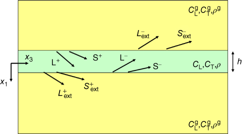
Figure 7.1 Example of sample geometry used in the partial wave technique. In each layer the partial waves (L±, S±) that combine to generate the guided wave are presented..
Source: © 2012 IEEE, reprinted, with permission, from Brum et al. [13]
The first step of the method consists in deriving the field equations for bulk waves, which are solutions to the wave equation in an infinite medium. As a result the stresses and displacements within the plate can be expressed in terms of the amplitudes of all the bulk waves that can exist within that plate. Then by introducing the proper boundary conditions at each interface the rules for coupling between plate and surrounding medium are defined. Finally, the different boundary conditions can be combined into one global matrix which describes the entire system by relating the bulk wave amplitudes to the physical constraints.
7.2.1 Field Equations for Plane Waves in Two Dimensions
In what follows it will be assumed that the wavelengths involved are smaller than the width of the plate and therefore a plane strain analysis is valid. The plane strain hypothesis restricts the model to waves whose particle motion is entirely in the (![]() ) plane, thus excluding for example shear horizontal (SH) modes. SH modes are usually not observed in ultrasound elastography since the ultrasound probe is placed parallel to the plate; however, they may be observed with other imaging modalities, such as MRI. (Please refer to references 11, 14, and 15 for further reading on SH modes and its inclusion into the general theory.)
) plane, thus excluding for example shear horizontal (SH) modes. SH modes are usually not observed in ultrasound elastography since the ultrasound probe is placed parallel to the plate; however, they may be observed with other imaging modalities, such as MRI. (Please refer to references 11, 14, and 15 for further reading on SH modes and its inclusion into the general theory.)
Under a plane strain hypothesis, where there is no variation of any quantity in the ![]() direction, the coordinate system may be reduced to the plane defined by the wave propagation direction and the normal to the plate (see Figure 7.1). A convenient way of presenting the solutions for bulk waves inside the plate is by introducing Helmholtz potentials. The longitudinal waves (L) are described by a scalar potential
direction, the coordinate system may be reduced to the plane defined by the wave propagation direction and the normal to the plate (see Figure 7.1). A convenient way of presenting the solutions for bulk waves inside the plate is by introducing Helmholtz potentials. The longitudinal waves (L) are described by a scalar potential ![]() while the shear waves (S) are described a vector potential
while the shear waves (S) are described a vector potential ![]() whose direction is normal to the wave propagation direction and the particle motion direction.
whose direction is normal to the wave propagation direction and the particle motion direction.
Here ![]() and
and ![]() are the longitudinal and shear wave amplitudes,
are the longitudinal and shear wave amplitudes, ![]() is the wavenumber vector, and
is the wavenumber vector, and ![]() is the angular frequency. From the potentials, the displacements of the longitudinal and shear waves can be calculated as
is the angular frequency. From the potentials, the displacements of the longitudinal and shear waves can be calculated as

7.2.2 The Partial Wave Technique in Isotropic Plates
As stated above, the development of a model for wave motion in plates is achieved by the superposition of longitudinal and shear bulk waves and the imposition of boundary conditions at the different interfaces. For modeling the guided wave propagating along the plate it is sufficient to assume the presence of four bulk waves inside the plate: two shear waves (![]() ) and two longitudinal waves (
) and two longitudinal waves (![]() ). Each of these bulk waves is termed a partial wave.
). Each of these bulk waves is termed a partial wave.
Let ![]() be denoted by
be denoted by ![]() , which corresponds to the wavenumber of the guided wave. Then, the
, which corresponds to the wavenumber of the guided wave. Then, the ![]() component of the wave vector of each partial wave can be expressed in terms of
component of the wave vector of each partial wave can be expressed in terms of ![]() and the bulk wave velocities of the plate as
and the bulk wave velocities of the plate as
where the subscript ![]() stands for the longitudinal or shear partial wave,
stands for the longitudinal or shear partial wave, ![]() denotes the bulk phase velocity of each type of wave in the plate and the + and − signs correspond to a wave moving with positive (“downward”) and negative (“upward”)
denotes the bulk phase velocity of each type of wave in the plate and the + and − signs correspond to a wave moving with positive (“downward”) and negative (“upward”) ![]() component. The displacements and stresses at any location inside the plate may be found from the amplitudes of the bulk waves using the field equations. In particular, the expressions for the two displacement components
component. The displacements and stresses at any location inside the plate may be found from the amplitudes of the bulk waves using the field equations. In particular, the expressions for the two displacement components ![]() and
and ![]() , the normal stress
, the normal stress ![]() , and the shear stress
, and the shear stress ![]() will be derived since in a plate system these quantities must be continuous over the different interfaces. From Hooke's law and the strain definition, the stresses can be calculated as
will be derived since in a plate system these quantities must be continuous over the different interfaces. From Hooke's law and the strain definition, the stresses can be calculated as


Thus for the longitudinal partial bulk waves it can be found
For the partial shear bulk waves
where ![]() ,
, ![]() , and
, and ![]() corresponds to the medium's density. The displacements and stresses at any location in the plate may be found by summing the contributions due to the four partial wave components.
corresponds to the medium's density. The displacements and stresses at any location in the plate may be found by summing the contributions due to the four partial wave components.

The matrix in Eq. (7.10) describes the relation between the wave amplitudes and the displacements and stresses at any position inside the plate. Its coefficients depend on the through‐thickness position inside the plate, i.e. ![]() ; the material properties of the layer, i.e.
; the material properties of the layer, i.e. ![]() ; and the frequency and wavenumber of the guided wave.
; and the frequency and wavenumber of the guided wave.
By using Eq. (7.10) it is possible to combine all the different boundary conditions at each interface into a single global matrix ![]() which represents the entire system [12]. The columns of the global matrix correspond to the amplitudes of the partial wave at each interface, while the rows correspond to each boundary condition. Thus, by multiplying the global matrix
which represents the entire system [12]. The columns of the global matrix correspond to the amplitudes of the partial wave at each interface, while the rows correspond to each boundary condition. Thus, by multiplying the global matrix ![]() by a vector
by a vector ![]() containing the partial wave amplitudes, all boundary conditions will be satisfied simultaneously. The resulting equation will always be zero providing the characteristic equation of the system
containing the partial wave amplitudes, all boundary conditions will be satisfied simultaneously. The resulting equation will always be zero providing the characteristic equation of the system
To obtain non‐trivial solutions for the vector of partial wave amplitudes ![]() , the determinant of the global matrix in Eq. (7.11) must be zero. This constraint will allow only particular wave numbers
, the determinant of the global matrix in Eq. (7.11) must be zero. This constraint will allow only particular wave numbers ![]() for a given frequency. By changing the frequency it is possible to find the relation
for a given frequency. By changing the frequency it is possible to find the relation ![]() , where
, where ![]() is the phase velocity of the guided wave, i.e. the phase velocity dispersion curve. The phase velocity dispersion curve is the quantity that is usually measured in ultrasound elastography. Consequently, to retrieve the bulk shear wave speed
is the phase velocity of the guided wave, i.e. the phase velocity dispersion curve. The phase velocity dispersion curve is the quantity that is usually measured in ultrasound elastography. Consequently, to retrieve the bulk shear wave speed ![]() and therefore the shear elasticity of the plate, it is necessary to fit the experimental dispersion curve to a given plate model. In what follows several plate models will be presented along with their different applications and consequences in ultrasound elastography.
and therefore the shear elasticity of the plate, it is necessary to fit the experimental dispersion curve to a given plate model. In what follows several plate models will be presented along with their different applications and consequences in ultrasound elastography.
7.3 Plate in Vacuum: Lamb Waves
Let us now apply Eq. (7.10) to study transverse wave propagation in an elastic plate in vacuum (i.e. Lamb waves). Although this situation is difficult to meet in practice it will be helpful to establish some basic concepts of guided wave propagation. These concepts will be used later in more complex situations. Let ![]() be the thickness of the plate. For a plate in a vacuum, the normal stresses should vanish at each interface (i.e. traction‐free condition):
be the thickness of the plate. For a plate in a vacuum, the normal stresses should vanish at each interface (i.e. traction‐free condition): ![]() at
at ![]() . Under this condition Eq. (7.10) results in
. Under this condition Eq. (7.10) results in

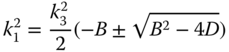
By combining rows and columns, the determinant of Eq. (7.12), which determines the phase velocity dispersion curve, gives

As described by Eq. (7.13), the determinant of the global matrix is calculated as a product of two determinants. Each determinant corresponds to one particular mode of propagation: the one on the left corresponds to the symmetric modes while the one on the right to corresponds to the anti‐symmetric modes. For the symmetric modes the longitudinal component of the displacement field (![]() ) is an even function of
) is an even function of ![]() while the transverse component (
while the transverse component (![]() ) is an odd function of
) is an odd function of ![]() . On the contrary, for the anti‐symmetric modes, while
. On the contrary, for the anti‐symmetric modes, while ![]() is an even function,
is an even function, ![]() is an odd function of
is an odd function of ![]() . Consequently, for each mode, the plate movement is either symmetric or anti‐symmetric with respect to the median plane of the plate. In Figure 7.2 the phase velocity dispersion curve along with a schematic of the plate movement is presented for the different modes. The anti‐symmetric and symmetric modes are denoted with letters
. Consequently, for each mode, the plate movement is either symmetric or anti‐symmetric with respect to the median plane of the plate. In Figure 7.2 the phase velocity dispersion curve along with a schematic of the plate movement is presented for the different modes. The anti‐symmetric and symmetric modes are denoted with letters ![]() and
and ![]() respectively, where the subscript
respectively, where the subscript ![]() . indicates the order of the mode.
. indicates the order of the mode.

Figure 7.2 (a) Wave velocity dispersion curves for an isotropic plate in vacuum presented in dimensionless variables c/c T and f·h/c T. The longitudinal wave speed was set to 1500 m/s. (b) Schematic of the plate displacement field for the first four modes for f·h/c T = 1.5.
By expanding each determinant in Eq. (7.13) the following characteristic equation is found for the symmetric (Eq. 7.14) and anti‐symmetric modes (Eq. 7.15) respectively
7.3.1 Low Frequency Approximation for Modes with Cut‐off Frequency
It may be observed in Figure 7.2 that several modes (![]() ) present a cut‐off frequency. Near the cut‐off frequency
) present a cut‐off frequency. Near the cut‐off frequency ![]() therefore
therefore ![]() ,
, ![]() and
and ![]() . Consequently, from Eq. (7.10), the displacement field and stresses near the cut‐off frequency may be expressed as
. Consequently, from Eq. (7.10), the displacement field and stresses near the cut‐off frequency may be expressed as
where the first term of each equation corresponds to the anti‐symmetric modes and the second to the symmetric modes. For the symmetric modes, the even solutions ![]() (
(![]() .) correspond to an even displacement field, therefore
.) correspond to an even displacement field, therefore ![]() . Consequently, the corresponding boundary condition gives
. Consequently, the corresponding boundary condition gives

This corresponds to a pure longitudinal symmetric mode. On the contrary, the odd solutions ![]() with
with ![]() ., correspond to
., correspond to ![]() , giving
, giving
which corresponds to a pure transverse mode. For the anti‐symmetric modes the same reasoning yields the following cut‐off frequencies
for the even (![]() .) and odd (
.) and odd (![]() .) anti‐symmetric modes respectively.
.) anti‐symmetric modes respectively.
At this point, it is important to notice the consequences of Eqs. (7.20)–(7.22) for Lamb wave propagation in soft tissues. In ultrasound elastography ![]() ∼ 1500 m/s,
∼ 1500 m/s, ![]() ∼ 1–20 m/s,
∼ 1–20 m/s, ![]() ∼ 1–20 mm, and the frequency is usually below 2 kHz. Therefore, the even anti‐symmetric and the odd symmetric modes will not be generated in an ultrasound elastography experiment since the lowest
∼ 1–20 mm, and the frequency is usually below 2 kHz. Therefore, the even anti‐symmetric and the odd symmetric modes will not be generated in an ultrasound elastography experiment since the lowest ![]() for these modes is ∼ 7.5 kHz (Eq. 7.21). On the contrary, the presence of the even symmetric modes and the odd anti‐symmetric modes will depend on frequency and on the ratio
for these modes is ∼ 7.5 kHz (Eq. 7.21). On the contrary, the presence of the even symmetric modes and the odd anti‐symmetric modes will depend on frequency and on the ratio ![]() (Eqs. 7.20 and 7.23). For tissues such as skin, arteries, bladder, or cornea where
(Eqs. 7.20 and 7.23). For tissues such as skin, arteries, bladder, or cornea where ![]() ∼ 1–3 mm, the
∼ 1–3 mm, the ![]() for these modes will lie in the kHz range and they will not be generated. Consequently, for these kind of tissues the only modes that may be expected are the zero‐order symmetric (
for these modes will lie in the kHz range and they will not be generated. Consequently, for these kind of tissues the only modes that may be expected are the zero‐order symmetric (![]() ) and anti‐symmetric (
) and anti‐symmetric (![]() ) modes, which have no cut‐off frequency. For other types of tissue, e.g. the myocardium, where
) modes, which have no cut‐off frequency. For other types of tissue, e.g. the myocardium, where ![]() ∼ 1 cm and
∼ 1 cm and ![]() ∼ 5 m/s, the cut‐off frequencies for
∼ 5 m/s, the cut‐off frequencies for ![]() is ∼250 Hz, for
is ∼250 Hz, for ![]() is ∼500 Hz, etc. Therefore, these modes may eventually coexist with the
is ∼500 Hz, etc. Therefore, these modes may eventually coexist with the ![]() and
and ![]() modes, depending on the type of source, frequency, plate thickness, and shear elasticity involved in the experiments. It is important to point out, that although these modes may theoretically be present, to our knowledge they have not been detected yet in a plate of soft tissue. This may be explained by the fact that, as seen above, the odd anti‐symmetric and symmetric modes are mainly longitudinal near the cut‐off frequencies, which, combined with a strong attenuation for frequencies above ∼400 Hz (i.e. tissue is by nature viscoelastic), makes it very difficult to detect them in the experiments. Consequently, the most common situation in an elastography experiment is the presence of the
modes, depending on the type of source, frequency, plate thickness, and shear elasticity involved in the experiments. It is important to point out, that although these modes may theoretically be present, to our knowledge they have not been detected yet in a plate of soft tissue. This may be explained by the fact that, as seen above, the odd anti‐symmetric and symmetric modes are mainly longitudinal near the cut‐off frequencies, which, combined with a strong attenuation for frequencies above ∼400 Hz (i.e. tissue is by nature viscoelastic), makes it very difficult to detect them in the experiments. Consequently, the most common situation in an elastography experiment is the presence of the ![]() and
and ![]() modes. Let us briefly present the main features of these modes.
modes. Let us briefly present the main features of these modes.
7.3.2 Modes Without Cut‐off Frequencies
In the low‐frequency approximation, i.e. as ![]() and
and ![]() approach to zero, Eq. (7.14) and Eq. (7.15) may be reduced to
approach to zero, Eq. (7.14) and Eq. (7.15) may be reduced to
From Eq. (7.24), the phase velocity for ![]() tends to a finite limit given by
tends to a finite limit given by ![]() , which for a soft tissue (
, which for a soft tissue (![]() ) may be approximated as
) may be approximated as ![]() . Additionally, it may demonstrated that when
. Additionally, it may demonstrated that when ![]() , the
, the ![]() mode is essentially longitudinal, i.e.
mode is essentially longitudinal, i.e. ![]() [15]. Since soft tissue is incompressible, a longitudinal displacement will generate a small but non‐negligible transverse displacement (see Figure 7.2b), therefore, this mode may be eventually detected by using ultrasound elastography. Additionally, the velocity of the mode is close to
[15]. Since soft tissue is incompressible, a longitudinal displacement will generate a small but non‐negligible transverse displacement (see Figure 7.2b), therefore, this mode may be eventually detected by using ultrasound elastography. Additionally, the velocity of the mode is close to ![]() and may be followed by an ultrafast scanner. For
and may be followed by an ultrafast scanner. For ![]() , by using Eq. (7.25), it may be demonstrated that its phase velocity may be approximated as
, by using Eq. (7.25), it may be demonstrated that its phase velocity may be approximated as
Therefore, by fitting this expression to the experimental dispersion curve the value of ![]() may be retrieved without cumbersome determinant calculations. In the high‐frequency region, i.e.
may be retrieved without cumbersome determinant calculations. In the high‐frequency region, i.e. ![]() , the velocities of the
, the velocities of the ![]() and
and ![]() approach to Rayleigh wave velocity which is ∼
approach to Rayleigh wave velocity which is ∼ ![]() . Therefore the phase velocity for the
. Therefore the phase velocity for the ![]() and
and ![]() modes will always lie between zero and
modes will always lie between zero and ![]() .
.
Finally, it is important to point out that the generation of each mode will not only depend on the frequency, but also on the type of source used in the experiments [11]. A type of source which is common in ultrasound elastography is the radiation force of ultrasound. This type of source acts all along the thickness of the plate in a direction perpendicular to the plate, generating mainly the ![]() mode, which is a flexural mode (Figure 7.2b).
mode, which is a flexural mode (Figure 7.2b).
7.4 Viscoelastic Plate in Liquid: Leaky Lamb Waves
Let us study a more realistic situation than a plate in vacuum. The model of a viscoelastic plate surrounded by non‐viscous fluid has widely been used to determine in vivo and ex vivo the shear elasticity and viscosity of several types of tissues, e.g. arteries [6, 7], cornea [1, 16, 17], bladder [5], and myocardium [3, 18]. In these works the Lamb waves were generated by using the acoustic radiation force of focused ultrasound, generating only ![]() mode. Therefore, in what follows, special attention will be devoted to this specific mode of propagation.
mode. Therefore, in what follows, special attention will be devoted to this specific mode of propagation.
7.4.1 Elastic Plate in Liquid
Let us derive the dispersion equation for an elastic plate in liquid by using the partial wave technique introduced in Section 7.2.2. For a plate embedded in a non‐viscous fluid of density ![]() and longitudinal wave velocity
and longitudinal wave velocity ![]() , six partial waves should be taken into account. The four waves inside the plate create two longitudinal waves (
, six partial waves should be taken into account. The four waves inside the plate create two longitudinal waves (![]() ,
, ![]() ) in the surrounding fluid. By applying the continuity at each interface of
) in the surrounding fluid. By applying the continuity at each interface of ![]() ,
, ![]() , and
, and ![]() the global matrix governing the system can be written as
the global matrix governing the system can be written as
where * denotes complex conjugate, ![]() , and
, and ![]() ,
, ![]() ,
, ![]() correspond to the surrounding liquid. By combining rows and columns the determinant of
correspond to the surrounding liquid. By combining rows and columns the determinant of ![]() may be calculated as a product of two sub‐determinants which give the following characteristic equations
may be calculated as a product of two sub‐determinants which give the following characteristic equations


Equations (7.28) and (7.29) correspond to the symmetric and anti‐symmetric modes respectively. It is important to notice that these equations differ from the equations for a plate in vacuum (Eqs. 7.14 and 7.15) by one term which takes into account the contribution of the fluid. In Figure 7.3 the phase velocity dispersion curves for the different modes for a plate in water (circles) are compared to the dispersion curves for a plate in vacuum (black dots).
Figure 7.3
Wave velocity dispersion curves for an isotropic plate in a non‐viscous fluid (i.e. leaky Lamb mode) shown in circles and a plate in vacuum shown in black dots. For both figures, (a) anti‐symmetric and (b) symmetric modes, 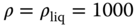 kg/m3 and
  m/s.
m/s.
7.4.1.1 Leakage into the Fluid
Contrary to what happens for a plate in a vacuum, where the acoustic energy is trapped inside the plate, for a plate surrounded by fluid the energy may leak into the surrounding medium. Leakage may be described by an amplitude exponential reduction with distance along the plate, which can be expressed by a complex wavenumber ![]() . The real part of the wavenumber is related to the phase velocity and describes the harmonic wave propagation while the imaginary part describes the wave attenuation in space.
. The real part of the wavenumber is related to the phase velocity and describes the harmonic wave propagation while the imaginary part describes the wave attenuation in space.
Leakage will depend on the ratio between the phase velocity of each mode and the bulk velocities of the plate. Snell's law requires that all the partial waves share the same frequency and spatial properties in the ![]() direction at each interface. This constrains the angles of incidence, transmission, and reflection of the partial waves inside the plate by
direction at each interface. This constrains the angles of incidence, transmission, and reflection of the partial waves inside the plate by

where ![]() are the angles at which longitudinal and shear partial waves propagate with respect to the
are the angles at which longitudinal and shear partial waves propagate with respect to the ![]() direction. Therefore, a leakage angle,
direction. Therefore, a leakage angle, ![]() , may be determined as
, may be determined as ![]() . Therefore, if
. Therefore, if ![]() , the leakage angle would be imaginary, which means that instead of creating a wave that propagates away from the plate, the displacements will decay exponentially and energy will be trapped in the fluid region close to the plate. [The same conclusion is obtained from Eq. (7.5): if
, the leakage angle would be imaginary, which means that instead of creating a wave that propagates away from the plate, the displacements will decay exponentially and energy will be trapped in the fluid region close to the plate. [The same conclusion is obtained from Eq. (7.5): if ![]() is smaller than
is smaller than ![]() then
then ![]() is imaginary and the wave is evanescent in the
is imaginary and the wave is evanescent in the ![]() direction.] Consequently, a mode will not leak if its phase velocity is less than the bulk velocity of any waves that can exist in the surrounding medium. In elastography, since
direction.] Consequently, a mode will not leak if its phase velocity is less than the bulk velocity of any waves that can exist in the surrounding medium. In elastography, since ![]() and
and ![]() , the phase velocities of the different measurable modes will be lower than
, the phase velocities of the different measurable modes will be lower than ![]() (see Figure 7.3) and no leakage should be considered. Therefore, when solving Eqs. (7.28) and (7.29) real values of
(see Figure 7.3) and no leakage should be considered. Therefore, when solving Eqs. (7.28) and (7.29) real values of ![]() should be searched.
should be searched.
7.4.2 Viscoelastic Plate
Another source of wave attenuation is viscosity, which is inherent to any type of tissue. In many applications viscosity had to be taken into account to properly model the guided wave propagation. To introduce viscosity, the elastic constant ![]() will no longer be considered as a real number but as a complex number instead. For example, if the frequency dependence is assumed to obey a Voigt model, as it was assumed in previous works [3, 9, 18], then
will no longer be considered as a real number but as a complex number instead. For example, if the frequency dependence is assumed to obey a Voigt model, as it was assumed in previous works [3, 9, 18], then ![]() may be written as
may be written as
where ![]() is the elastic component and
is the elastic component and ![]() is the viscous component or viscosity. [Other rheological models, such as Maxwell or Zener, will introduce different relations than the one presented in Eq. (7.31); please refer to Fung [19] for further details.] It is important to note that the partial wave technique still remains valid in the presence of viscosity [12]; however, to solve Eqs. (7.28) and (7.29) complex wavenumbers
is the viscous component or viscosity. [Other rheological models, such as Maxwell or Zener, will introduce different relations than the one presented in Eq. (7.31); please refer to Fung [19] for further details.] It is important to note that the partial wave technique still remains valid in the presence of viscosity [12]; however, to solve Eqs. (7.28) and (7.29) complex wavenumbers ![]() should be searched: the real part is related to the phase velocity and the imaginary part is related to wave attenuation. In Figure 7.4 the phase velocity and attenuation dispersion curves for different values of viscosity are presented. In this figure
should be searched: the real part is related to the phase velocity and the imaginary part is related to wave attenuation. In Figure 7.4 the phase velocity and attenuation dispersion curves for different values of viscosity are presented. In this figure ![]() , with Re[ ] being the real part.
, with Re[ ] being the real part.

Figure 7.4 (a) Phase velocity and (b) attenuation dispersion curves for the A0 mode in a viscoelastic plate in water for different values of viscosity η.
From Figure 7.4, it is important to point out, that while the phase velocity dispersion curve differs from the pure elastic case (the solid line) for values of f·h/c T > 0.15, for f·h/c T < 0.1 they practically remain unchanged when viscosity is added. On the other hand, the attenuation dispersion curve is clearly sensitive to viscosity. This effect has already been observed by Nguyen et al. [2] for Lamb waves in viscoelastic isotropic plates and by Brum et al. [9] for guided wave propagation in the Achilles tendon. Consequently, for low values of f·h/c T, the elasticity constant associated with the guided wave can be retrieved directly from the phase velocity dispersion curve independently of the viscosity effects, i.e. elasticity and viscosity are uncoupled.
7.4.3 Empirical Formula
An empirical formula (Eq. 7.32) was first proposed by Couade et al. [6] to retrieve the shear modulus of the arterial wall from the ![]() dispersion curve by assuming the artery to behave as an elastic plate in water.
dispersion curve by assuming the artery to behave as an elastic plate in water.

This formula introduces a correction factor of ![]() when compared to the low‐frequency approximation of the
when compared to the low‐frequency approximation of the ![]() mode for a plate in vacuum (Eq. 7.26).
mode for a plate in vacuum (Eq. 7.26).
The validity of this empirical formula was discussed in the work of Nguyen et al. [2] in the case of thin elastic plates submerged in water. In this work, Eq. (7.32) was tested for plate thicknesses and shear wave speeds ranging between 0.5 and 1.5 mm and 5 and 10 m/s respectively, showing that the relative deviation of the empirical formula from simulated dispersion curves is as much as 15% for the thickest and softest plates. However, its deviation was less than 5% for plates of 1 mm thickness whose shear wave speeds were greater than 10 m/s. Therefore, this empirical formula is suitable for some particular applications, e.g. elasticity estimation of cornea, skin, or the arterial wall.
7.5 Isotropic Plate Embedded Between Two Semi‐infinite Elastic Solids
The model of an isotropic plate surrounded by two semi‐infinite elastic solids of bulk waves speed ![]() and
and ![]() has been used in vitro by Brum et al. [13] to measure the elasticity of thin plates embedded in an elastic solid and numerically by Couade et al. [6] to establish the bias of the Leaky lamb model used in their work with respect to other plate models with more realistic boundaries conditions.
has been used in vitro by Brum et al. [13] to measure the elasticity of thin plates embedded in an elastic solid and numerically by Couade et al. [6] to establish the bias of the Leaky lamb model used in their work with respect to other plate models with more realistic boundaries conditions.
For a plate embedded in an elastic medium eight partial waves should be taken into account (see Figure 7.1). The four waves inside the plate create two kinds of waves in the surrounding medium: one shear and one longitudinal wave propagating with positive (![]() ,
, ![]() ) and negative (
) and negative (![]() ,
, ![]() )
) ![]() component. As a consequence at each interface six partial waves should be taken into account. By applying the continuity at each of the interfaces of
component. As a consequence at each interface six partial waves should be taken into account. By applying the continuity at each of the interfaces of ![]() ,
, ![]() ,
, ![]() , and
, and ![]() the global matrix governing the system can be written as
the global matrix governing the system can be written as
For the equation of ![]() ,
, ![]() , and
, and ![]() with a superscript
with a superscript ![]() with
with ![]() , the bulk wave speeds and density of each semi‐infinite solid should be used. For the particular case of
, the bulk wave speeds and density of each semi‐infinite solid should be used. For the particular case of ![]() , Brum et al. [13] demonstrated that the determinant of
, Brum et al. [13] demonstrated that the determinant of ![]() may be reduced to a product of two determinants
may be reduced to a product of two determinants

The determinant on the left corresponds to the anti‐symmetric modes and the one on the right to the symmetric modes. Since the plate is embedded in an elastic medium, leakage will occur whenever the phase velocity of the guided wave ![]() exceeds one of the bulk wave velocities of the surrounding medium. Since in elastography
exceeds one of the bulk wave velocities of the surrounding medium. Since in elastography ![]() , leakage will mainly depend whether
, leakage will mainly depend whether ![]() is greater or less than the shear wave speed of the surrounding medium. Therefore, complex wavenumbers should be searched when solving Eq. (7.34).
is greater or less than the shear wave speed of the surrounding medium. Therefore, complex wavenumbers should be searched when solving Eq. (7.34).
7.6 Transverse Wave Propagation in Anisotropic Viscoelastic Plates Surrounded by Non‐viscous Fluid
Transverse isotropic tissue like tendons and muscles are commonly present in ultrasound elastography. Recently, guided wave propagation along a transverse isotropic plate has been used to model shear wave propagation in vivo in the human Achilles tendon [9, 10]. Another example lies in the cornea [17]. Let us briefly describe the main features of guided wave propagation along transverse isotropic plates.
For an isotropic solid only two constants (i.e. Lamé constants) are needed to characterize it. On the contrary, for a transverse isotropic solid the Christoffel's tensor ![]() describing the system is composed of five independent elastic constants:
describing the system is composed of five independent elastic constants: ![]() ,
, ![]() ,
, ![]() ,
, ![]() , and
, and ![]() . In an infinite transverse isotropic medium the elastic constants
. In an infinite transverse isotropic medium the elastic constants ![]() ,
, ![]() , and
, and ![]() can be determined from the measurement of longitudinal ultrasound phase velocities along the perpendicular and parallel directions, respectively. Moreover, the elastic constants
can be determined from the measurement of longitudinal ultrasound phase velocities along the perpendicular and parallel directions, respectively. Moreover, the elastic constants ![]() and
and ![]() can be deduced from the phase velocity measurement of shear waves propagating either parallel or perpendicular to the fibre direction with a polarization perpendicular to the fibers [20]. However, in a transverse isotropic plate the relation between phase velocity and elasticity is more complex. Let us use the partial wave technique to derive the secular equation for a transverse isotropic plate. Two situations will be considered:
can be deduced from the phase velocity measurement of shear waves propagating either parallel or perpendicular to the fibre direction with a polarization perpendicular to the fibers [20]. However, in a transverse isotropic plate the relation between phase velocity and elasticity is more complex. Let us use the partial wave technique to derive the secular equation for a transverse isotropic plate. Two situations will be considered: ![]() parallel and perpendicular to the fiber orientation.
parallel and perpendicular to the fiber orientation.
7.6.1 Guided Wave Propagation Parallel to the Fibers
Let us first consider the case where the wave propagation direction is parallel to the fibers. A plane wave traveling in an arbitrary direction x may be written as
where ![]() is the displacement vector and
is the displacement vector and ![]() is its amplitude. Under a plane strain condition, the nature of the bulk plane waves which can exist within a transverse isotropic plate are determined by Christoffel's equation
is its amplitude. Under a plane strain condition, the nature of the bulk plane waves which can exist within a transverse isotropic plate are determined by Christoffel's equation

Thus, by combining Eq. (7.35) and Eq. (7.36), the following equations relating the plane wave amplitudes ![]() and
and ![]() are deduced
are deduced
From Eq. (7.37) it is possible to express the ratio R between the wave amplitudes ![]() and
and ![]() as
as

By eliminating ![]() and
and ![]() from Eq. (7.38) by using Eq. (7.39), the following quadratic equation for
from Eq. (7.38) by using Eq. (7.39), the following quadratic equation for ![]() in terms of
in terms of ![]() and the elastic constants is deduced
and the elastic constants is deduced
where ![]() and
and ![]() are given by
are given by
Let us define ![]() and
and ![]() as the two values of
as the two values of ![]() obtained from Eq. (7.40) with + and – signs respectively. Also,
obtained from Eq. (7.40) with + and – signs respectively. Also, ![]() and
and ![]() will denote the value of
will denote the value of ![]() when
when ![]() and
and ![]() are respectively substituted in Eq. (7.39).
are respectively substituted in Eq. (7.39).
The equations above, derived for bulk plane waves propagating in an unbounded transverse isotropic medium, predict the presence of four partial waves. These partial waves are the equivalent of the two shear and the two longitudinal partial waves described in the case of an isotropic plate described in Section 7.2. Consequently, the displacements inside the plate may be written as a superposition of partial waves
where the subscript i = p,m stands for the partial wave propagating with wave number component ![]() and
and ![]() respectively. By coupling these displacements along with the stresses (σ
11 = C
11(∂u
1/∂x
1) + C
13(∂u
3/∂x
3) and σ
13 = C
13(∂u
1/∂x
3 + ∂u
3/∂x
1) to the ones of the surrounding fluid, the global matrix gives
respectively. By coupling these displacements along with the stresses (σ
11 = C
11(∂u
1/∂x
1) + C
13(∂u
3/∂x
3) and σ
13 = C
13(∂u
1/∂x
3 + ∂u
3/∂x
1) to the ones of the surrounding fluid, the global matrix gives

where X = e ikp.h/2, Y = e ikm.h/2, G p,m = C 11 k p,m + C 13 R p,m .k, H p,m = R p,m k p,m + k. By combining columns and rows, the determinant of the global matrix can be calculated as follows

The determinant on the left corresponds to the anti‐symmetric modes while the one on the right corresponds to the symmetric modes. This determines the dispersion relation for the different modes of a wave propagating along a transverse isotropic elastic plate in a direction parallel to the fibers. In this case the velocity dispersion curve will depend on following elastic constants: ![]() ,
, ![]() ,
, ![]() , and
, and ![]() . To introduce viscosity, the elastic constant
. To introduce viscosity, the elastic constant ![]() should be considered as complex number.
should be considered as complex number.
7.6.2 Guided Wave Propagation Perpendicular to the Fibers
To solve the problem of guided wave propagation in the direction perpendicular to the fibers it is important to note that this is the same problem of wave propagation along the parallel direction but in a different reference frame. Thus, it suffices to change the subscript 3 to 2 and replace C 55 by C 66 in Eqs. (7.39) to (7.42) to re‐obtain Eq. (7.46). However, since the plate is transverse isotropic: C 11 = C 22 and C 12 = C 11 – 2C 66. Under these conditions H p,m, G p,m, and k p,m are reduced to the following expressions
Consequently Eq. (7.46) may be reduced to Eqs. (7.28) and (7.29), which corresponds to the Leaky Lamb wave equation for an isotropic plate of shear wave speed of (C 66/ρ)1/2 and longitudinal wave speed of (C 11/ρ)½. Again, to introduce viscosity C 66 may be considered to obey a Voigt model, thus, C 66 = c 66 + iη 66.
7.7 Conclusions
Throughout this chapter the main features of transverse wave propagation in plate structures with application to ultrasound elastography have been reviewed. Wave propagation in such a configuration may be described as a superposition of different modes of propagation (e.g. symmetric/anti‐symmetric modes) which depend on the geometry, isotropy, mechanical properties, and boundary conditions of the wave guide. Moreover, the generation of each mode will depend on the frequency and type of source used in the experiments. In this scenario, it is mandatory to take the dispersive nature of each mode into account in order to retrieve the shear wave speed of the plate, otherwise bias in the shear wave speed estimation will be introduced. For a given application, once a plate model is assumed (e.g. plate in water, plate in vacuum, etc.) the shear wave speed of the plate may be retrieved by identifying the corresponding mode and fitting the theoretical dispersion curve to the experimental data. At the moment, the only mode that was consistently detected using ultrasound elastography is the zero ‐order anti‐symmetric mode. However, new applications will shortly lead to the detection of other types of modes as well as to the development of the theory for different types of geometries, sources, wave guides, etc.
Acknowledgments
The author would like to thank Dr. Nicolás Benech, Dr. Carlos Negreira, and Dr. Xiaoping Jia for the interesting discussions on guided wave generation and propagation. Javier Brum is supported by PEDECIBA‐Física, Uruguay and Agencia Nacional de Investigación e Innovación (ANII), Uruguay.
References
- 1 Tanter, M., Touboul, D., Gennisson, J.L., et al. (2009). High‐resolution quantitative imaging of cornea elasticity using supersonic shear imaging. IEEE Trans. Med. Imaging 28: 1881–1893.
- 2 Nguyen, T.M., Couade, M., Bercoff, J., and Tanter, M. (2011). Assessment of viscous and elastic properties of sub‐wavelength layered soft tissues using shear wave spectroscopy: theoretical framework and experimental in vitro experimental validation. IEEE Trans. Ultrason., Ferroelectr., Freq. Control 58: 2305–2315.
- 3 Nenadic, I.Z., Urban, M.W., Aristizabal, S., et al. (2011). Lamb wave dispersion ultrasound vibrometry (LDUV) method for quantifying mechanical properties of viscoelastic solids. Phys. Med. Biol. 56: 2245–2264.
- 4 Urban, M.W., Pislaru, C., Nenadic, I., et al. (2013). Measurement of viscoelastic properties of in vivo swine myocardium using Lamb wave dispersion ultrasound vibrometry (LDUV). IEEE Trans. Med. Imaging 32: 247–261.
- 5 Nenadic, I.Z., Qiang, B., Urban, M.W., et al. (2013). Ultrasound bladder vibrometry method for measuring viscoelasticity of the bladder wall. Phys. Med. Biol. 58: 2675–2695.
- 6 Couade, M., Pernot, M., Prada, C., et al. (2010). Quantitative assessment of arterial wall biomechanical properties using shear wave imaging. Ultrasound Med. Biol. 36: 1662–1676.
- 7 Bernal, M., Nenadic, I., Urban, M.W., and Greenleaf, J.F. (2011). Material property estimation for tubes and arteries using ultrasound radiation force and analysis of propagating modes. J. Acoust. Soc. Am. 129: 1344–1354.
- 8 Dutta, P., Urban, M., Le Maitre, O., et al. (2015). Simultaneous identification of elastic properties, thickness, and diameter of arteries excited with ultrasound radiation force. Phys. Med. Biol. 60: 5279–5296.
- 9 Brum, J., Bernal, M., Gennisson, J.L., and Tanter, M. (2014). In vivo evaluation of the elastic anisotropy of the human Achilles tendon using shear wave dispersion analysis. Phys. Med. Biol. 59: 505–523.
- 10 Helfenstein‐Didier, C., Andrade, R.J., Brum, J., et al. (2016). In vivo quantification of the shear modulus of the human Achilles tendon during passive loading using shear wave dispersion analysis. Phys. Med. Biol. 61: 2485–2496.
- 11 Auld, B.A. (1973). Acoustics Fields and Waves in Solids, Vol. 2. New York: Wiley.
- 12 Lowe, M. (1995). Matrix techniques for modelling ultrasonic waves in multi‐layered media. IEEE Trans.Ultrason., Ferroelectr., Freq. Control 42: 525–542.
- 13 Brum, J., Gennisson, J.L., Nguyen, T.M., et al. (2012). Application of 1D transient elastography for the shear modulus assessment of thin layered soft tissue: comparison with supersonic shear imaging technique. IEEE Trans. Ultrason., Ferroelectr., Freq. Control 59: 703–714.
- 14 Graff, K.F. (1975). Wave Motion in Elastic Solids. New York: Dover Publications.
- 15 Royer, D. and Dieulesaint, E. (1996). Elastic Waves in Solids I: Free and Guided Propagation. Berlin: Springer.
- 16 Nguyen, T.M., Aubry, J.F., Toubul, D., et al. (2012). Monitoring of cornea elastic properties chnages during UV‐A/riboflavin‐induced corneal collagen cross‐linking using supersonic shear wave imaging: a pilot study. Invest. Ophthalmol. Vis. Sci. 53: 5948–5954.
- 17 Nguyen, T.M., Aubry, J.F., Fink, M., (2013). In vivo evidence of porcine cornea anisotropy using supersonic shear wave imaging. Invest. Ophthalmol. Vis. Sci. 55: 7545–7552.
- 18 Nenadic, I.Z., Urban, M.W., Mitchell, S.A., and Greenleaf, J.F. (2011). On Lamb and Rayleigh wave convergence in viscoelastic tissues. Phys. Med. Biol. 56: 6723–6738.
- 19 Fung, Y.C. (1993). Biomechanics: Mechanical Properties of Living Tissues. New York: Springer.
- 20 Royer, D., Gennisson, J.L., Deffieux, T. and Tanter, T. (2011). On the elasticity of transverse isotropic soft tissues. J. Acoust. Soc. Am. 129: 2757–2760.