
14
Intrinsic Cardiovascular Wave and Strain Imaging
Elisa Konofagou
Department of Biomedical Engineering, Columbia University, New York, NY, USA
14.1 Introduction
Cardiovascular diseases remain America's primary killer by a large margin, claiming the lives of more Americans than the next two main causes of death combined (cancer and pulmonary complications). In particular, coronary artery disease (CAD) is by far the most lethal, causing 17% of all deaths every year (whether cardiac related or not). One of the main reasons for this high death toll is the severe lack of effective and accessible imaging tools upon anomaly detected on the electrocardiogram (ECG), especially at the early stages when CAD can be stabilized with appropriate pharmacological regimen. Arrhythmias refer to the disruption of the natural heart rhythm. Cardiac arrhythmias lead to a significant amount of cardiovascular morbidity and mortality. An irregular heart rhythm causes the heart to suddenly stop pumping blood. Atrial pathologies are the most common arrhythmias, with atrial fibrillation and atrial flutter being the most prevalent. Similarly, arterial stiffening has been linked to a variety of diseases – spanning from cardiovascular disease and dementia to Parkinson's, diabetes, and end‐stage renal disease. Yet, in sharp contrast with the clear universality and significance of pulse waveform velocity (PWV) as a biomarker, is the lack of such measurements in the clinic. There is currently no technique that yields a regional PWV or maps the PWV along a detected pathology to evaluate risk. This is because current methodology assumes a single stiffness value over the entire circulation obtained through a carotid‐to‐femoral pressure measurement. Clearly, this single stiffness value is not sufficient to localize or characterize focal disease such as aneurysms or atherosclerotic plaques. In this chapter, we introduce ultrasound‐based methodologies that are based on inferring the mechanical and electrical properties of the myocardium as well as mechanical properties of the vascular wall in order to better image the onset and progression of the aforementioned diseases.
14.2 Cardiac Imaging
14.2.1 Myocardial Elastography
14.2.1.1 Introduction
According to the latest report on Heart Disease and Stroke Statistics by the American Heart Association [1], more than 2150 Americans die of cardiovascular disease each day, an average of 1 death every 40 seconds. Cardiovascular disease currently claims more lives each year in both men and women than the next two most deadly diseases combined, i.e. cancer and chronic lower respiratory disease. Among the cardiovascular diseases, coronary artery disease (CAD) is by far the most deadly, causing approximately 1 of every 6 deaths in the United States in 2010. Approximately every 34 seconds, one American has a coronary event, and approximately every 1 minute 23 seconds, an American will die of one. It is estimated that an additional 150 000 silent first myocardial infarctions occur each year [1]. However, there are currently no screening or early detection imaging techniques that can identify abnormalities prior to any symptoms or fatalities. Clinically available imaging techniques such as echocardiography or nuclear perfusion (radionuclide imaging) are typically used after a cardiac event has already occurred to determine the extent of damage. Despite the fact that over the past few years therapeutic techniques, such as angioplasty, heart valve surgery, and pacemakers, have experienced exponential growth in new procedures, the progress in the development of novel diagnostic techniques has stalled by comparison.
14.2.1.2 Mechanical Deformation of Normal and Ischemic or Infarcted Myocardium
Detection of cardiac dysfunction through assessment of the mechanical properties of the heart, and more specifically, the left‐ventricular muscle, has been a long‐term goal in diagnostic cardiology. This is because both ischemia [2], i.e. the reduced oxygenation of the muscle necessary for its contraction, and infarction [3], i.e. the complete loss of blood supply inducing myocyte death, alter the mechanical properties and contractility of the myocardium. In the ischemic heart, the diastolic left‐ventricular pressure–volume or pressure–length curve slope is typically increased, suggesting increased chamber stiffness [4]. Regional myocardial stiffness has also been reported to increase as a result of ischemia [5–8]. The increased stiffness could be due to myocardial remodeling, including elevated collagen and desmin expression as well as the titin isoform switch [4]. Acute myocardial infarction caused by partial or total blockage of one or more coronary arteries can cause complex structural alterations of the left‐ventricular muscle [9]. These alterations may lead to collagen synthesis and scar formation, which can cause the myocardium to irreversibly change its mechanical properties. Holmes et al. [10] reported that this myocardial stiffening can be measured within the first 5 minutes following ischemic onset. As reported by Gupta et al. [9], in vitro mechanical testing showed that the stiffness of the infarcted region increases within the first 4 hours, and continues to rise by up to 20 times, peaking 1–2 weeks following the infarct and decreasing 4 weeks later (down to 1–10 times the non‐infarcted value). The fact that the mechanical properties induced by the ischemia change right at the onset, continue changing thereafter, and peak two weeks later, indicate the potential for a mechanically based imaging technique to detect the ischemia and infarct extent early. Regarding its conduction pattern, ischemia or infarction will alter the normal pattern and result in reduced and complete lack of conduction, respectively, at the region of abnormality since the myocytes no longer properly conduct the action potential.
14.2.1.3 Myocardial Elastography
Our group has pioneered the technique of myocardial elastography that we have been developing for more than a decade [11–18]. This technique encompasses imaging of mechanical (cumulative or systolic; Figure 14.1) or electromechanical (incremental or transient) strain or activation times to respectively highlight the mechanical or electrical function of the myocardium. Myocardial elastography benefits from the development of techniques used for high precision 2D time‐shift‐based strain estimation [19] and high frame rates available in echocardiography scanners [13] to obtain a detailed map of the transmural strain in normal [20–22], ischemic [21], and infarcted [23] cases in vivo. These strain‐imaging techniques aim at achieving high precision estimates through recorrelation techniques [19] and customized cross‐correlation methods [24] and are thus successful in mapping the full 2D and 3D strain tensors [18, 25, 26].

Figure 14.1 (a) Envisioned role and (b, c) initial findings of myocardial elastography in the current clinical routine to avoid false positives and/or thus unnecessary invasive procedures and false negatives by the currently used techniques. (b) Normal short‐axis radial strain image, largely thickening myocardium, in an echocardiography false positive case where CT angiography was administered only to confirm normal function. (c) Abnormal short‐axis radial strain image containing an ischemic region (thinning; arrow) in a nuclear perfusion. Subsequent CT angiography confirmed the myocardial elastography findings regarding two occluded territories (64‐year‐old female, 40% LAD and 30% RCA occlusion). (d) Coronary territories given for reference. CUMC: Columbia University Medical Center. LAD: left anterior descending artery, LCx: left circumflex artery, RCA: right coronary artery. Myocardial Elastography was capable of detecting normal function and identifying both compromised territories.

Figure 14.2 (a) B‐mode, (b) radial, (c) circumferential, and (d) longitudinal strain images of a cylindrical model undergoing radial deformation using PBME in phased array configuration in FIELD II for 2D (top panel) and 3D (bottom panel) myocardial elastography. In the proposed study, the canine LV geometry and electromechanical simulation model (Figure 14.3) are used. The black boundaries in the top panel represent where the simulated myocardium. Strains outside the tissue are not taken into account.
14.2.1.3.1 2D Strain Estimation and Imaging
A fast, normalized cross‐correlation function is first used on RF signals from consecutive frames to compute two‐dimensional motion and deformation [19, 27]. The cross‐correlation function uses a 1D kernel (length = 5.85 mm, overlap = 90%) in a 2D (or 3D) search to estimate both axial and lateral (and elevational) displacements (Eq. 14.1; Figures 14.1 and 14.2). The correlation kernel size is approximately 10 wavelengths, which has been found to be the optimal length using cross‐correlation [28]. It should also be noted that the elastographic resolution has been shown to depend mainly on the kernel shift (not the kernel size) [29], which in our studies is 10%, or 0.6 mm. When searching in the lateral (or, elevational) direction, the RF signals are linearly interpolated by a factor of 10 in order to improve lateral (or, elevational) displacement [19, 21, 30]. Recorrelation techniques are applied in two iterations that aim at increasing the correlation coefficient of each strain component by correction or shifting the RF signals by the displacements estimated in the other (two) orthogonal direction(s) [19, 30]. A least‐squares kernel [31] is finally applied to compute the axial and lateral strains in 2D‐PBME (parallel beamforming myocardial elastography) and axial, lateral, and elevational strains in 3D‐PBME. The estimated displacements use a reference point of the first frame in each estimation pair, yielding incremental (inter‐frame) strains that are then accumulated over the entire systolic phase. Radial, circumferential, and longitudinal strains are then calculated. For 2D, radial and circumferential strains are estimated in a short‐axis view (Figures 14.2b and 14.2c). In 2D‐PBME, rotation matrices, ![]() , for each material point within the myocardium in a 2D short axis view are written as
, for each material point within the myocardium in a 2D short axis view are written as

where ![]() is the angle relative to the origin of the Cartesian coordinates in the FE models. Strains in cardiac coordinates are therefore obtained by
is the angle relative to the origin of the Cartesian coordinates in the FE models. Strains in cardiac coordinates are therefore obtained by
where ![]() is the 2D radial‐circumferential strain tensor. The diagonal components of
is the 2D radial‐circumferential strain tensor. The diagonal components of ![]() are radial (
are radial (![]() ) and circumferential (
) and circumferential (![]() ) strains. Positive and negative radial strains indicate myocardial thickening and thinning, respectively, while myocardial stretching and shortening are represented by positive and negative circumferential strains, respectively. A standard B‐mode image (Figure 14.2a) is reconstructed from the RF data, allowing for manually initialized segmentation of the myocardial border, which is subsequently automatically tracked throughout the cardiac cycle based on the estimated displacements – as previously developed by our group [27].
) strains. Positive and negative radial strains indicate myocardial thickening and thinning, respectively, while myocardial stretching and shortening are represented by positive and negative circumferential strains, respectively. A standard B‐mode image (Figure 14.2a) is reconstructed from the RF data, allowing for manually initialized segmentation of the myocardial border, which is subsequently automatically tracked throughout the cardiac cycle based on the estimated displacements – as previously developed by our group [27].
14.2.1.3.2 3D Strain Estimation and Imaging
3D includes the estimation of longitudinal strains. The MATLAB function interp3 is used to interpolate all three orthogonal components (axial, lateral, radial, and circumferential) between each of the 16 slices. The interpolated data set is depicted in 3D, on two surfaces: one located near the endocardium, the other located near the epicardium. The frame rate is lower by 16‐fold compared to 2D, i.e. 344 frames/s in 3D (from 5500 frames/s in 2D) but is tested whether it can be sufficient to estimate strain at high signal to noise ratio (SNR) as predicted by preliminary findings (Figure 14.3).

Figure 14.3 E(SNRe|ε) transverse strain curves increase with frame rate.
14.2.1.3.3 PBME Performance Assessment
A probabilistic framework has been developed by our group in order to compare the strain estimation quality between conventional and parallel beamforming [23, 32]. The elastographic signal‐to‐noise‐ratios (SNRe) are calculated for each sequence over the phase of systole. SNRe is computed for every point in an image using
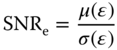
where μ(ε) and σ(ε) refer to the mean and standard deviation of the strain (ε) magnitude within a small 2D region of interest (ROI) (3.0 × 3.2 mm). Since both strain and SNRe are computed for each point in the myocardium throughout systole, a large number (>600 000) of strain‐SNRe pairs are generated for each sequence [23]. The conditional expected values of SNRe for each strain are calculated using [23, 32]

E(SNR e |ε) curves are generated for each sequence, which allows for a relatively easy comparison to be performed between different sequences for a wide range of strain values. Examples of E(SNRe|ε) curves for radial strain estimation are provided in Figure 14.3. The SNRe of both 2D‐PBME and 3D‐PBME are computed with respect to the strain (equivalent to frame rate) and compared to focused (standard 2D and 3D myocardial elastography) to perform a quality comparison with parallel beamforming techniques. Both inter‐frame (electromechanical) and cumulative (mechanical) strain SNRe are quantified.
14.2.1.3.4 Compounding
A compounding technique is applied to determine increase in SNR when parallel beamforming is applied. Plane waves are electronically steered and transmitted at three different angles separated by 20° (–20°, 0°, 20°) and the resulting RF frames are combined into a compounded image. The received radiofrequency (RF) frames are reconstructed by applying a delay‐and‐sum method on GPU‐based parallel computing to accelerate reconstruction processing [32]. In preliminary studies, we have found that compounding in human hearts in vivo decreases the frame rate from 5500 fps to 1375 fps, which is sufficiently high for myocardial elastography (Figure 14.3) while SNR increases by 4‐fold.
14.2.1.4 Simulations
A phased array simulation model was implemented for the quality assessment of PBME. Field II, an established and publicly available ultrasound field simulation program [33, 34] is used to simulate the RF signals of the myocardium. The simulated mesh, including the myocardium, cavity, and background are loaded into FIELD II [28, 35]. Instead of a focused wave, a diverging wave sequence is employed for transmit by placing the focus 6.75 mm (half the size of the aperture) behind the array surface to achieve a 90° angle insonification [32]. For 2D‐PBME, the RF signals are obtained from 192 elements and 3.5 MHz center frequency with 60% bandwidth (at −6dB) phased array similar to those used in the canine study. Hanning apodization is applied both during transmit and receive to reduce grating lobes. The width and height of the phased array are 43 and 7 mm, respectively. The RF signals are reconstructed by coherent summation of the signals received by all the elements using a delay‐and‐sum algorithm. For 3D‐PBME, RF signals are obtained from a 2D array with 16 × 16, 32 × 32, and 64 × 64 elements and 3 MHz center frequency, similar to those used in experiments.
14.2.1.5 Myocardial ischemia and infarction detection in canines in vivo
14.2.1.5.1 Ischemic Model
In order to test myocardial elastography in the assessment of ischemia by depicting the change in both mechanical and electrical properties, twelve (n = 12) adult male dogs (20–25 kg) were used according to well‐established anesthetized canine models. The flow in the coronary artery was continuously controlled via pressure‐flow curves.
- Step 1 (control): Mongrel dogs with normal/healthy myocardium, as verified using standard echocardiography, are used for control measurements. Channel data with both 2D‐ and 3D‐PBME are continuously acquired during 5 min in sets of three cardiac cycles each taken 20 s apart, i.e. approximately 15 sets in total. This established the strain baseline.
- Step 2 (mild to acute ischemia): The dogs undergo a left thoracotomy followed by gradual constriction of the mid‐proximal left anterior descending coronary artery (LAD) using the Ameroid constrictor by 0–100% of baseline, at intervals of 20% for 15 min each. Strain images are shown in Figure 14.4a. The slope of the coronary pressure‐flow curves (using Millar catheters and sonomicrometry) are used to monitor the ischemic onset at each occlusion step. RF data in the same views as in Step 1 were continuously acquired during the full 15 min in sets of three cardiac cycles (10 s apart), i.e. approx. 70 sets total.

Figure 14.4 (a) Progression of ischemia, shown as thinning systolic strain as indicated compared to the surrounding non‐ischemic (thickening) strain, from 0% to 100% occlusion in the same dog using 2D‐PBME and identifying the region and extent of ischemia in each case (shown with the ROI). (b) TTC pathology showing pale (unstained by TTC; ischemic) vs. red (stained by TTC; normal) myocardium. (c) Temporal radial strain profiles in the anterior wall region of 3 × 3 mm2 at 0%, 40%, 60%, and 100% occlusion levels with sonomicrometry (SM) and 2DME [21].
14.2.1.5.2 Infarct Model
Mongrel dogs underwent similar surgical procedure as in the ischemia model but survived for four days after complete ligation only in order to develop a fully developed infarct (Figure 14.5).

Figure 14.5 (a) Transthoracic systolic radial strain image of a canine left ventricle in vivo. Thinning strain region clearly indicates the extent of infarction. (b) Electromechanical isochrones in 3D identifying spatial extent of MI. Arrow denotes MI region.
14.2.1.6 Validation of Myocardial Elastography against CT Angiography
CT angiography is an established technique used for reliable detection of a coronary occlusion and was used to confirm the occlusion and validate the location of the ischemia or infarct as detected by myocardial elastography. The objectives of this study were to show that 2D myocardial strains can be imaged with diverging wave imaging and are different in average between healthy subjects and coronary artery disease (CAD) patients. In this study, 15 CAD patients and 8 healthy subjects were imaged with ME. Patients with more than 50% occlusion in one of the main coronary arteries were considered to have obstructive CAD. Incremental axial and lateral displacements were estimated using normalized 1D cross‐correlation and then accumulated during systole. Axial and lateral cumulative strains were then estimated from the displacements and converted to radial cumulative strains (Figures 14.6 and 14.7). The end‐systolic radial strain in the total cross‐section of the myocardium in healthy subjects (14.9 ± 8.2%) was significantly higher than obstructive CAD patients (−0.9 ± 7.4%, p < 0.001) and in non‐obstructive CAD patients (3.7 ± 5.7%, p < 0.05). End‐systolic radial strain in the left anterior descending (LAD) territory was found to be significantly higher in healthy subjects (16.9 ± 12.9%) than in patients with obstructed LAD (2.2 ± 7.0%, p < 0.05) and patients with non‐obstructed LAD (1.7 ± 10.3%, p < 0.05) (Figure 14.8). These findings indicate that end‐systolic radial strain measured with myocardial elastography is higher on average in healthy subjects compared to CAD patients and indicates that myocardial elastography has the potential to be used for non‐invasive, radiation‐free early detection of CAD.

Figure 14.6 Comparison between (a) 2D‐ME (conventional (focused) beamforming) using ECG gating and (b) 2D‐PBME (parallel beamforming) systolic radial strain image in a normal patient. The quality is comparable without the artifacts from sector matching and ECG gating in part (a).

Figure 14.7 2D‐PBME showing progression of coronary disease in three different patients: (a) Normal; (b) occlusions – RCA: 90%; LAD: 20%, LCX: 20%; and (c) occlusions – RCA: 99%; LAD: 100%, LCX: 100%. Figure 14.1d can be used for reference of the position of the coronary arteries.
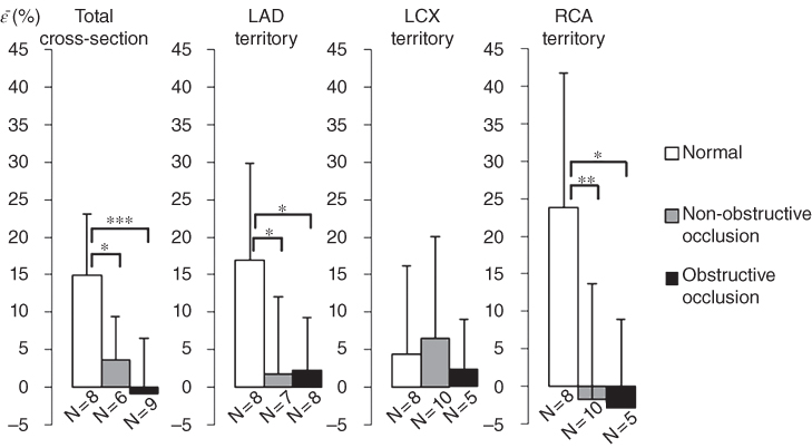
Figure 14.8 Preliminary findings in 25 human subjects (19 patients and 6 normals) using PBME. Non‐severe CAD (stenosis <50%) and severe (>50% stenosis). LAD: left anterior descending artery; LCx: left‐circumflex artery; RCA: right coronary artery; total: all territories. In all territories except LCx PBME was capable of differentiating normal from non‐severe and from severe CAD.
14.2.2 Electromechanical Wave Imaging (EWI)
14.2.2.1 Cardiac Arrhythmias
Cardiac arrhythmias can be separated into atrial (or supraventricular) and ventricular. While ventricular arrhythmias, such as ventricular fibrillation (chaotic rhythm), ventricular tachycardia (rapid rhythm), and ventricular bradycardia (slow rhythm) incur the most episodes of sudden death, they are less common and easier to diagnose than atrial arrhythmias. Atrial arrhythmias, including atrial fibrillation (Afib or AF) and atrial flutter (AFL), are the most common. Similar to the ventricular definition, atrial fibrillation denotes the chaotic rhythm while atrial flutter denotes the regular but abnormal (rapid or slow) rhythm. The number of individuals with atrial fibrillation in the United States is expected to reach 12 million by 2050 [36] with atrial flutters, often a result of treatment, also expected to rise as more of these treatments are administered. The EWI methodology has the dual purpose of both enhancing the diagnosis and treatment planning and guidance of arrhythmias that are both the most common but also the most difficult to diagnose, i.e. the atrial arrhythmias. A short overview of the state‐of‐the‐art diagnostic and treatment techniques is provided.
14.2.2.2 Clinical Diagnosis of Atrial Arrhythmias
ECG recordings and no imaging modality is typically used for the noninvasive identification of atrial arrhythmias. If ECG recordings indicate atrial flutter or fibrillation, Radio‐frequency (RF) ablation (see Section 14.2.2.3) is warranted that allows for catheterized cardiac mapping during its procedure. Cardiac mapping involves the insertion of a catheter containing a small number of electrodes in the heart chamber to contact the endocardium and measure times of activation. The procedure is minimally invasive and ionizing since it uses computed tomography (CT) guidance, but it can be a lengthy procedure requiring topical or general anesthesia and is warranted only when the ECG recordings indicate that RF ablation is the appropriate course of treatment. Limitations include some inaccessible endocardial sites and the inability to map the mid‐myocardium and epicardium. More importantly, as potentials in only one or a few locations in the atrium are measured per heartbeat it can be used only to study stable, repeatable arrhythmias.
14.2.2.3 Treatment of Atrial Arrhythmias
Radio‐frequency ablation is a minimally invasive technique rapidly emerging as the most commonly used therapeutic modality for atrial flutter and atrial fibrillation. For this treatment, a catheter, whose tip carries an electrode, is inserted through the femoral vein and the tip of the electrode is positioned at the arrhythmic origin. The tip causes a frictional heat generated by intracellular ions moving in response to an alternating current. The electrode is connected to a function generator and the electrical current flows and raises the local temperature up to 95 °C, maintaining it for about 15 min, generating thermal lesions in the vicinity of the ablating catheter. The treatment consists thus in modifying or blocking the circuits of electrical conduction in the heart. Current surgical procedures are invasive and have a moderate efficiency in the persistent forms of atrial fibrillation. AF in some patients may be due to focal activity originating in the pulmonary veins and 70% of these patients can be successfully treated by RF ablation of the focus inside the pulmonary veins [37]. However, the treatment of AF using RF ablation can often lead to the development of other arrhythmias. For example, a sizeable increase of atypical flutter is due to catheter ablation of atrial fibrillation.
14.2.2.4 Electromechanical Wave Imaging (EWI)
14.2.2.4.1 Cardiac Electromechanics
The heart will not adequately contract unless it is electrically activated via a very specific route (Figure 14.9; green arrows). In sinus rhythm (that is, natural contraction), the path of activation originates at the sinoatrial (SA) node (right before the ECG's P‐wave), from which the electrical signal in the form of an action potential spreads to both right and left atria causing their contraction (during the P‐wave). The wave then propagates to the atrioventricular (AV) node (right after the P‐wave), through the bundle of His and along the left and right bundles on the interventricular septum (during the Q‐R segment) to the Purkinje fibers (S‐wave) finally causing both ventricles to synchronously contract, starting at the apex towards their lateral and posterior walls (Figure 14.9). The heart is thus an electromechanical pump that needs to first be electrically activated in order to contract. Propagating electrical waves of excitation result in localized contractions. Each electrical activation in Figure 14.9b is followed by an electromechanical one, i.e. the depolarization of a cardiac muscle cell, or, myocyte, is followed by an uptake of calcium, which triggers contraction after a certain electromechanical delay of a few milliseconds [38, 39]. In the presence of arrhythmia, electrical and electromechanical patterns are disrupted.

Figure 14.9 (a) State‐of‐the‐art CT angiography of the CRT leads. The ablation catheters and coronary arteries are clearly visible but the heart and the myocardium are not visible. A similar system is used to guide electroanatomic mapping. (b) Illustration of the cardiac conduction system. The arrows indicate the path of activation as the action potential propagates from the sinoatrial node (SA node) in the right atrium along the Purkinje fiber network. (c) Current (2D) 4‐chamber EWI activation map with conventional beamforming in a normal human heart obtained transthoracically. (d) 3D‐rendered, 4‐chamber EWI activation map (reversed color map used compared to part c) in vivo.
14.2.2.4.2 Electromechanical Wave Imaging (EWI)
Our group has pioneered a unique noninvasive and direct (as opposed to inverse problem) imaging technique that could reliably map the conduction wave in the heart in all of its four cardiac chambers. Electromechanical wave imaging [15, 16, 20, 40–48] has been shown capable of noninvasively mapping the conduction wave during propagation. We identified that high frame rate (>500 frames/s, fps) and precise 2D imaging of the cardiac deformation is feasible so that the transient cardiac motion resulting from the fast electromechanical wave can be mapped in murine [15, 16, 40–43], canine [20, 46–48], and human [15, 32, 45] hearts in vivo. We were also capable of demonstrating that EWI is angle‐independent [47], has excellent correlation with electrical activation measurements in canines in vivo [47] (slope of 0.99 and r 2 = 0.88; Figures 14.10 and 14.11) and is in excellent agreement with electromechanical simulations [32, 49]. More importantly, our group was capable of recently showing that EWI was feasible in the atria of human hearts in vivo undergoing sinus rhythm. [32]. There is simply no other modality that can directly map the conduction of the atria under sinus rhythm noninvasively in the clinic. An important additional advantage of this methodology is that it can be routinely applied in the clinic through straightforward integration with any echocardiography system. It could thus be used both at the diagnostic and at the treatment guidance levels, either off‐ or on‐line. Despite the fact that EWI can map both the atria and the ventricles, we chose to focus on the atrial arrhythmias in this study given that they are far more common, more salvageable, and completely lacking of any noninvasive imaging modality that can map their conduction properties.

Figure 14.10 (a) Propagation of the electromechanical wave when paced from the lateral wall, near the base. Activation in this view corresponds to thickening of the tissue. Activated regions are traced at (A) 15 ms, (B) 30 ms, (C) 50 ms (D) 85 ms, and (E) 120 ms and indicated on the electrocardiogram (F). 0 ms corresponds to the pacing stimulus. A–C: The EW propagates from the basal part of the lateral wall towards the apex. D: Note that in the apical region, a transition from lengthening to shortening is observed rather than a transition from thinning to thickening. D, E: In the anterior wall, the EW propagates from both the base and apex. The scale shows inter‐frame strains. (b) Correlation of EWI with simulation findings of electromechanical and electrical activation [46]. (c) Electrical and electromechanical activation times during the four pacing protocols and sinus rhythm in four different heart segments in the posterior and anterior walls [46].
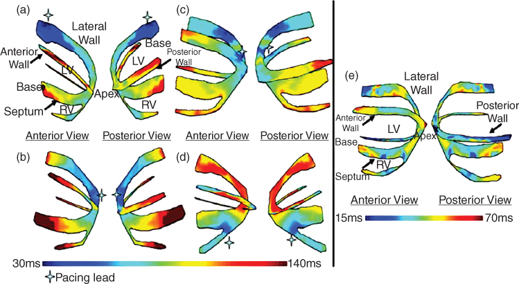
Figure 14.11 Isochrones showing the activation sequence under different pacing protocols as shown. Arrow indicates the pacing origin. (a) Pacing from the basal region of the lateral wall; (b) pacing from the apex; (c) pacing from the apical region of the lateral wall; (d) pacing from the apical region of the right‐ventricular wall; and (e) Isochrones showing the EW activation sequence during sinus rhythm. The activation sequence exhibits early activation at the median level and late activation at the basal and apical levels. Activation of the right ventricular wall occurred after the activation of the septal and lateral walls. The cross indicates the pacing lead location.
EWI can be useful in a number of diseases that can be treated with ablation therapy: e.g. atrial fibrillation, atrial flutter, ventricular tachycadia, Wolff‐Parkinson‐White (WPW) syndrome, etc. WPW is a heart condition where an additional electrical pathway links the atria to the ventricles. It is the most common heart rate disorder in infants and children and is preferably treated using catheter ablation. EWI could be used in predicting the location of the accessory pathway, thus reducing the overall time of the ablation procedure. Since a sizeable increase of atypical flutter is due to catheter ablation of atrial fibrillation, the prevalence of atrial flutter is also expected to rise. However, the relationship between AF and AFL is still not fully understood [50]. Atrial flutter, a type of atrial tachycardia, has historically been defined exclusively from the ECG recordings. More specifically, differentiation between flutter and other tachycardias was based on the atrial rate and the presence or absence of isoelectric baselines between atrial deflections. Since then, electrophysiological studies and RF ablation brought new understanding into the atrial tachycardia mechanisms, which did not correlate well with these ECG‐based definitions [51]. In other words, ECG recordings offer only a limited value in the determination of specific atrial tachycardia mechanisms, and, ultimately, for the selection of the appropriate course of treatment. Cardiac mapping allowed different mechanisms of macroreentrant atrial tachycardia to be identified, such as typical flutter, reverse typical flutter, left atrial flutter, etc., although a significant number of atypical flutters are still poorly understood [51, 52]. While mapping the right atrium is routinely undertaken successfully using this procedure, mapping the left atrium is riskier since it requires a transseptal puncture. However, as it currently stands in the clinic, right atrium arrhythmia cannot be distinguished from left atrium arrhythmia prior to treatment and only the latter warrants transseptal puncture, which is a riskier procedure. In some cases, the left atrium arrhythmia is not diagnosed until the entire right atrium is ablated (which may involve several unproductive hours of intervention), posing further risk to the patient. Consequently, left atrial activation sequences are not well characterized in many atrial tachycardia cases [51]. Moreover, the surface ECG is insufficiently specific to distinguish left from right atrial flutters [50, 52]. EWI could thus offer an important step for the localization of the right vs. left atrial arrhythmia as well as localizing the origin(s) at the treatment planning stage, i.e. prior to the catheterization of the patient rendering the treatment to be more efficient, much shorter in duration, and with unnecessary ablations in the wrong chamber or avoiding unnecessary transseptal punctures.
14.2.2.4.3 Treatment Guidance Capability of EWI
Currently, there is simply no noninvasive electrical conduction mapping techniques of the heart that can be used in the clinic. In addition, apart from the currently available clinical electrical mapping methods being all catheter‐based and limited to mapping the endocardial or epicardial activation sequence, they are also time‐consuming and costly. Even in a laboratory setting, mapping the 3D electrical activation sequence of the heart can be a daunting task [53]. Studies of transmural electrical activation usually require usage of a large number of plunge electrodes to attain sufficient resolution [54–56], or are applied to small regions of interest in vivo [38]. Non‐contact methods to map the electrical activation sequence have also emerged but are not used in the clinic. Optical imaging techniques use voltage‐sensitive dyes that bind to cardiac cell membranes and, following illumination, fluoresce if the cell undergoes electrical activation. Optical imaging methods can map the activation sequence of ex vivo tissue on the endocardial and epicardial surfaces [57–62] but cannot be applied in the clinic since they require the use of an electromechanical decoupler that inhibits cardiac contraction during imaging. Other newly developed methods to map the local electrical activity of the heart based on inverse problems are available: electrocardiographic imaging (ECGI) [63–65] and non‐contact mapping [66–68]. The former is based on body surface potentials and CT or MRI scans and provides reconstructed epicardial action potentials, including the atria [69]. The latter consists in reconstructing the transmural potentials from potentials measured in the heart chamber based on specific assumptions that may be susceptible to inverse problem errors [70–72].
14.2.2.5 Imaging the Electromechanics of the Heart
As of today, no imaging method currently used in the clinic has been capable of mapping the electromechanics of the heart. Initial measurements to determine the correlation between the electrical and electromechanical activities have been reported [73, 74]. These results suggest that the electrical activation sequence could be deduced from the electromechanics. Clinically available imaging modalities, such as standard echocardiography or MRI, cannot adequately detect the electromechanical wave (EW) since they are too slow, i.e. the time required to acquire a single image is similar to the duration of the entire ventricular depolarization. The electrical activation lasts approximately 60 to 100 ms and requires a resolution of a few milliseconds (e.g. 2–5 ms) to generate precise activation maps. Moreover, the regional inter‐frame deformation to be measured at these frame rates is very small (∼0.25% at a 2 ms temporal resolution) and requires a highly accurate strain estimator [20, 46–48]. We have shown that EWI is capable of reaching high frame rates (up to 2000 frames/s) as well attain the precision of the incurred strains (up to 0.25%) which result from an electromechanical activation and therefore fulfill the requirements of both high temporal and spatial resolution unique to our technology.
14.2.2.6 EWI Sequences
A block diagram of EWI is shown in Figure 14.12. Two imaging sequences, the automated composite technique (ACT) [45] and the temporally‐unequispaced acquisition sequences (TUAS) [32, 75] have been developed and implemented [20, 32, 46–48, 75–77] as well as the single‐heartbeat sequence [32, 75–79].

Figure 14.12 Block diagram of the EWI technique. (a) High frame‐rate acquisition is first performed using either ACT (follow lighter arrows) or TUAS (black arrows). (b) High precision displacement estimation between two consecutively acquired RF beams (t 1, t 2) is then performed using very high frame rate RF speckle tracking. (c) In ACT only, a region of the heart muscle, common to two neighboring sectors, is then selected. By comparing the temporally varying displacements measured in neighboring sectors (s 1, s 2) via a cross‐correlation technique, the delay between them is estimated. (d) In ACT only, a full‐view ciné‐loop of the displacement overlaid onto the B‐mode can then be reconstructed with all the sectors in the composite image synchronized. (e) In ACT and TUAS, the heart walls are then segmented, and incremental strains are computed to depict the EW. (f) By tracking the onset of the EW, isochrones of the sequence of activation are generated.
14.2.2.6.1 The ACT Sequence
An Ultrasonix RP system with a 3.3 MHz phased array was used to acquire RF frames from 390 to 520 frames/s (fps) using an automated composite technique (ACT) [45]. Briefly, to increase the resulting frame rate, the image is divided into partially overlapping sectors corresponding to separate cardiac cycles (Figure 14.12a). The axial incremental displacements are obtained with a RF‐based cross‐correlation method (Figure 14.12b) (window size: 4.6 mm, 80% overlap). Briefly, this method consists in dividing every ultrasound beam in a large number of overlapping, one‐dimensional, 4.6 mm‐long windows. Then, the following process is applied to each window and each sampled time t. A reference window at time t 1 is compared with all the windows contained in the same beam at sampled time t 2. The axial location of the window providing the highest correlation determines the axial displacement between two consecutive sampled times. After repeating this process for every available window and every available sampled time, we obtain axial displacements at multiple locations along the ultrasound beam and for every sampled time. The full‐view image is then reconstructed using the motion‐matching technique (Figure 14.12c) [20]. Briefly, this method consists of comparing, through a cross‐correlation method, the incremental displacements measured in the overlapping line of two sectors obtained at different heartbeats to synchronize the sectors. More specifically, the acquisition sequence is designed such that each sector contains at least one ultrasound beam that is also part of the following sector. Therefore, this overlapping beam is expected to result in identical (or highly similar) axial displacements whether they corresponds to heartbeat h that occurred when sector s was acquired or to heartbeat h + 1 that occurred when sector s + 1 was acquired. By comparing, over time, the displacements obtained in the overlapping beams, the time delay corresponding to the maximum cross‐correlation coefficient are obtained to synchronize each set of neighboring sectors. The procedure is repeated for each pair of sectors, allowing the reconstruction of the full‐view of the heart, hence ensuring the continuity of the transition incremental displacements across sectors. This method does not rely on the ECG. Therefore it is especially useful in cases where the ECG may be unavailable or too irregular to perform ECG gating [20]. The axial incremental strains were then obtained by taking the spatial derivative of incremental strains in the axial direction using a least‐squares estimator [31] with a kernel equal to 6.75 mm (Figure 14.12d). The myocardium was segmented using an automated contour tracking technique [80] and displacement and strain maps were then overlaid onto the corresponding B‐mode images (Figure 14.12e). Isochrones were generated by mapping the first time occurrence at which the incremental strains crossed zero following the Q‐wave. More specifically, the absolute value of the incremental strains was minimized in a temporal window following the Q‐wave in up to a hundred manually selected regions. Noisy data were excluded. Subsample resolution was obtained through spline interpolation and Delaunay interpolation was used to construct continuous isochronal maps. Two echocardiographic planes, identical to the planes imaged in the standard apical four‐ and two‐chamber views, were imaged across the long axis of the heart. These two views were temporally co‐registered using the ECG signals, spatially co‐registered by an echocardiography expert, and displayed in a three‐dimensional biplane view in Amira 4.1 (Visage Imaging, Chelmsford, MA) (Figure 14.12f).
14.2.2.6.2 The TUAS Sequence
We have developed and implemented in an Ultrasonix MDP system a temporally unequispaced acquisition sequence (TUAS) (Figure 14.12) [32], which is a sector‐based sequence [81], adapted to optimally estimate cardiac deformations. In TUAS, it is possible to simultaneously achieve a wide range of frame rates for motion estimation, large beam density, and a large field of view in a single heartbeat, thus avoiding the motion‐matching and reconstruction steps in EWI, with little dependence on depth and beam density. Consequently, for a given set of imaging parameters, motion can be estimated at frame rates varying from a few Hz to kHz. The prior knowledge, in this case, is the minimum sampling rate, i.e. the Nyquist rate, of the motion over time at a given pixel. The conventional way to construct an ultrasound image using a phased array is to acquire a finite number of beams, typically 64 or 128, over a 90° angle. These beams are acquired sequentially, and the process is repeated for each frame. For example, a given beam, e.g. beam 3 (Figure 14.13), is acquired at a fixed rate (Figure 14.13, conventional sequence). In TUAS, the beam acquisition sequence is reordered to provide two distinct rates, defined as follows (Figure 14.13): the motion‐estimation rate and the motion‐sampling rate. The motion‐estimation rate r me is defined as the inverse of the time, i.e. T me, lapsing between the two RF frames used to estimate motion. The motion‐sampling rate rms is defined as the inverse of the time, i.e. T ms, lapsing between two consecutive displacement maps. In conventional imaging sequences, these two rates are equal, because a given frame is typically used for two motion estimations (un and un + 1 in Figure 14.13). In TUAS, the operator can adjust the motion‐estimation rate. As shown in Figure 14.13, a frame in the TUAS case is used only once for motion estimation, thus halving the motion‐sampling rate relative to the conventional method. For example, an acquisition performed at a 12 cm depth with 64 beams with a conventional sequence corresponds to a frame rate of 100 Hz. However, while 100 Hz may suffice to satisfy the Nyquist sampling criterion of cardiac motion, it is usually insufficient for accurate motion tracking using RF cross‐correlation. Therefore, to reach a higher frame rate of, e.g. 400 Hz typically used for EWI, the conventional sequence requires to divide the number of beams by four, and thus reduce either the beam density, the field of view, or both. At the same depth and beam density, TUAS provides a motion‐sampling rate of 50 Hz and a motion‐estimation rate that can be varied, as shown in the following section, within the following group: {6416, 3208, 1604, 802, 401, 201, 100} Hz. This has numerous advantages. For example, both the beam density and the field of view can be maintained while estimating the cardiac motion with an optimal frame rate, which could be, e.g. either 401 or 802 Hz, depending on the amplitude of the cardiac motion. This results into a halving of the motion‐sampling rate; however, the motion‐sampling rate has only little effect on the motion estimation accuracy. Theoretically, if this rate remains above the Nyquist rate of the estimated cardiac motion, it will have no effect. We estimated that at a motion‐sampling rate above 120 Hz, the effect of the motion‐sampling rate became negligible compared to the effect of the motion‐estimation rate [32].
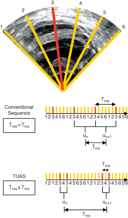
Figure 14.13 Illustration of an acquisition sequence in a simple case where only six lines form an image, with each sector using two lines. In a conventional acquisition sequence, the time separating two acquisitions of the same line is the same. In TUAS, the time separating two acquisitions of the same line is modulated to optimize motion estimation.

Figure 14.14 Distribution of strains during the EW for different motion‐estimation rates. Conditional probability density function of the SNRe knowing the strain value (and the corresponding motion‐estimation rate). The conditional expectation values of SNRe, the ZZLB, BB, and CRLB are also displayed.
14.2.2.6.3 Single‐heartbeat EWI and Optimal Strain Estimation
In TUAS, a wide range of frame rates can be achieved, including very high frame rates, independently of other imaging parameters. Therefore, by maintaining a set of imaging parameters (e.g. field of view, imaging depth) and varying the frame rate, it is possible to identify an optimal frame rate by studying the link between the strain signal‐to‐noise ratio (SNRe) and the EW. A previous report [82] on the strain filter indicates that the SNRe depends mostly on the value of the strains to be measured when the imaging parameters are fixed. This theoretical framework allows the construction of an upper limit on the SNRe as a function of the strain amplitude (also known as the strain filter). The strain filter corresponds, in this case, to the Ziv‐Zakai lower bound (ZZLB) on the variance. The ZZLB is a combination of the Cramér‐Rao lower bound (CRLB) and the Barankin bound (BB). The ZZLB transitions from the CRLB to the BB when decorrelation becomes important to the point that only the envelope of the signal contains information on the motion [83]. In the correlation model used here [84], this transition occurs only at very large strains. Since the amplitude of strains to be measured is directly related to the motion‐estimation rate (a large motion‐estimation rate will result in small inter‐frame strains), finding an optimal strain value is equivalent to finding an optimal motion‐estimation rate. The strain filter was calculated with the imaging parameters used in this study as a reference; however, it was developed for the analysis of strains occurring in static elastography and is not adapted to the more complex motion of the heart. We have therefore developed a new probabilistic framework based on experimental data acquired in a paced canine in vivo to not only establish an upper bound on the SNRe, but to estimate the probability of obtaining a given SNRe for a given strain amplitude [32]. Since the motion‐estimation rate can be used as a means to translate and narrow the strain distribution), the optimal motion‐estimation rate can be found by studying the link between the strains and the SNRe. More specifically, a conditional probability density function spanning a large range of strains values was constructed (Figure 14.14) and was found in agreement with the strain‐filter theory, which provides a higher bound on the SNRe. The ZZLB predicts a sharp transition between the CRLB and BB when decorrelation becomes important, to the point that the phase of the signal does not contain information about motion. Figure 14.14 shows that the conditional probability density function is comprised within the CRLB up to approximately 4% before it becomes comprised within the BB. A sharp decrease in the expected value of the SNRe is also observed at 4% strain, underlining the importance of using the phase information of the RF signal for accurate strain measurements. A distortion in the strain distribution may indicate that while a high SNRe can be maintained, the accuracy of the strain estimator is strongly impaired at low motion‐estimation rates, i.e. less than 350 Hz in this case (Figure 14.14). Finally, we showed that TUAS is capable of accurately depicting non‐periodic events at high temporal resolution. Therefore, the optimal frame rate will need to be between 389 and 3891 Hz according to the strains estimated (Figure 14.14). Strain patterns expected during such a phenomenon were depicted, such as a disorganized contraction, leading to little to no large scale motion of the heart. Regions of the myocardium were oscillating rapidly from thinning to thickening and thickening to thinning over time. Studying the frequencies of these oscillations could be useful in understanding the mechanisms of fibrillation [85] and we plan to use Fourier‐based analysis and principal component analysis in order to identify those components in fibrillation and better identify the arrhythmic origin(s). Ciaccio et al. [86] have developed such methods, including non‐harmonic analysis for the analysis of electrical signals in the heart during fibrillation (and will assist in further development for EWI).
14.2.2.7 Characterization of Atrial Arrhythmias in Canines In Vivo
14.2.2.7.1 Electrical Mapping
Data from the St. Jude EnSite system was exported to a workstation for co‐registration with EWI isochrones. Comma separated value (CSV) files containing the coordinates of the 3D mesh as well as the data from each acquired point (activation time and spatial coordinates) were retrieved. The 3D mesh was recreated in Maya (Maya 2016, Autodesk, San Rafael, CA, USA) and the open‐source software MeshLab (Visual Computing Lab – ISTI, CNR, meshlab.sourceforge.net). 3D co‐registration was performed by aligning the isochrones with the 3D mesh using anatomical landmarks such as the location of the apex, the mitral valve annulus, the lateral wall, or the septum. Once both the isochrones and the mesh were aligned, positions of the acquired points on the EnSite system were projected onto the isochrones and times of activation were compared. This process provided pairs of electrical and electromechanical activation times which were then plotted against each other. Linear regression was then performed and slope, intercept, and R 2 values were obtained.
14.2.2.7.2 Validation
The objective of this study was to validate EWI against electrical mapping using an electroanatomical mapping system, in all four chambers of the heart. Six (n = 6) normal adult canines were used in this study. The electrical activation sequence was mapped in all four chambers of the heart, both endocardially and epicardially using a St. Jude EnSite mapping system (St. Jude Medical, Secaucus, NJ). EWI acquisitions were performed during normal sinus rhythm and pacing and isochrones of the electromechanical activation were generated. Electromechanical and electrical activation times were plotted against each other and linear regression was performed for each pair of activation maps. Electromechanical and electrical activations were found to be highly correlated with slopes of the correlation ranging from 0.77 to 1.83, electromechanical delays between 9 and 58 ms and R 2 values from 0.71 to 0.92 (Figure 14.15). The excellent linear correlation between electromechanical and electrical activation and good agreement between the activation maps indicate that the electromechanical activation follows the pattern of propagation of the electrical activation. This suggests that EWI could be used to accurately characterize arrhythmias and localize their source.

Figure 14.15 Comparison of EWI against electroanatomical mapping. Anterior and posterior views in the (a) right (RA) and left (LA) atria and (b) entire canine left ventricle (LV) using EWI noninvasively and electroanatomical mapping with the proposed clinical system (Ensite, St. Jude Medical). Linear regression analysis shows excellent correlation between the electromechanical and electrical activation with the intercept indicating the electromechanical delay [79].
14.2.2.8 EWI in Normal Human Subjects and with Arrhythmias
The objectives of the clinical studies [23, 32, 46–48, 77] were (i) to determine the potential for clinical role of EWI, by predicting activation patterns in normal subjects, (ii) to determine the feasibility of EWI to identify the site of origin in subjects with tachyarrhythmia, and (iii) to identify the myocardial activation sequence in patients undergoing CRT. In normal subjects (Figures 14.16 and 14.17), the EW propagated, in both the atria and the ventricles, in accordance with the expected electrical activation sequences based on reports in the literature. In subjects with CRT, EWI successfully characterized two different pacing schemes, i.e. LV epicardial pacing and RV endocardial pacing versus sinus rhythm with conducted complexes. In two subjects with AFL (Figure 14.18), the propagation patterns obtained with EWI were in agreement with results obtained from invasive intracardiac mapping studies, indicating that EWI may be capable of distinguishing LA from RA flutters transthoracically. Finally, we have shown the feasibility of EWI to describe the activation sequence during a single heartbeat in a patient with AFL and RBBB (Figure 14.18) [32]. The results presented demonstrate for the first time that mapping the transient strains occurring in response to the electrical activation, i.e. the electromechanical wave propagation, can be used to characterize both normal rhythm and arrhythmias in humans, in all four cardiac chambers transthoracically using multiple‐ and single‐heartbeat methodologies. EWI has the potential to noninvasively assist in clinical decision making prior to invasive treatment, and to aid in optimizing and monitoring responses to CRT. Some more recent endeavors are using multi‐2D rendering for reconstruction of the ventricular [87] and atrial surfaces.

Figure 14.16 EWI using a flash sequence for motion estimation (motion sampling rate: 2000 Hz, motion estimation rate: 500 Hz) overlaid on a standard 128‐beams, 30‐fps B‐mode. All four chambers are mapped but only atrial activation is shown here. Activation (shortening) was initiated in the right atrium (RA) (50 ms) and propagated towards the atrial septum (60 ms) and the left atrium (LA) (70 ms) until complete activation of both atria (100 ms). RV: right ventricle, LV: left ventricle.

Figure 14.17 EWI isochrone in all four chambers in a healthy, 23‐year‐old male subject. Activation in this view corresponds to shortening of the tissue. Activation is initiated in the right atrium and propagates in the left atrium. After the atrio‐ventricular delay, activation is initiated in the ventricles from multiple origins, which are possibly correlated with the Purkinje terminal locations. Arrows (both white and black) indicate the direction of propagation.

Figure 14.18 Noninvasively detecting and characterizing atrial flutter with EWI in three human subjects (RA: right atrium, LA: left atrium). (a) Normal subject: activation is initiated in the right atrium and propagates towards the left atrium. (b) Unknown atrial flutter in a flutter patient with a prosthetic mitral valve, which was believed to cause the atrial flutter from the left side. Since the patient could not sustain the long procedure needed to construct a full activation map using cardiac mapping, ablation was attempted without complete information in two locations in the left atrium, which did not lead to cardioversion, i.e. did not return to sinus rhythm. The patient was sent home and a second ablation is scheduled in the near future. This case exemplifies the need for a faster mapping method, which could have led to the proper identification of the ablation site and so potentially limit the number of ablation procedures needed to treat this patient. Indeed, the EWI isochrones shown here display the initial activation in the left atrium, close to the septum. (c) Atypical left atrial flutter patient confirmed by cardiac mapping. EWI isochrones also show early activation is initiated in the left atrium. (d) CARTO map of a left‐sided flutter case.
14.3 Vascular Imaging
14.3.1 Stroke
Stroke is one of the leading causes of death often associated with severe, long‐term disability [88]. One of the main reasons behind this large death toll is that characterization of plaque composition in the clinic remains a remarkable challenge with no real consensus and no noninvasive modalities, as MRI, CT, and ultrasound currently fall short for different reasons [89]. In addition, approximately 795 000 people in the United States suffer new strokes every year [1]. About 20–30% of new strokes are attributed to atherosclerotic carotid artery disease, i.e. approximately 200 000 per year [90]. Atherosclerotic plaques are characterized by a focal accumulation of lipids, complex carbohydrates, blood cells, fibrous tissues, and calcified deposits [91]. Currently, despite major advances in the treatment of atherosclerosis, a large percentage of individuals with the disease die without any prior symptoms [92].
14.3.2 Stroke and Plaque Stiffness
The development of carotid plaques has been generally associated with local changes in the vascular mechanical properties [91]. However, none of the aforementioned modalities provide any mechanical property information. Biomechanical studies have been conducted to assess lesion morphology while the tissue properties are related to the tissue stresses and the vulnerability of the plaque. For example, using 2D finite element analysis (FEA), the presence of a lipid pool has been shown to increase the tissue stress in the overlying fibrous cap compared to a fibrous core [93]. Based on the assumption that decreasing the cap thickness could increase the risk of rupture [94], the effect of the cap thickness was investigated experimentally. A criterion was thus proposed with caps smaller than 65 µm prone to rupture in coronaries [95, 96], while in carotids this critical cap thickness was found to be higher (200 µm) [97]. However, it has been observed that thicker caps can also rupture, the rupture can occur at stresses lower than the predicted threshold of 300 kPa, and the ruptures frequently do not coincide with the location of peak circumferential stress [98]. Therefore, additional parameters are warranted as determinants of plaque rupture in addition to the cap thickness [99]. A large histological study has evidenced that the composition of the plaque is correlated to the vulnerability [97]. Furthermore, Lee et al [100] demonstrated the radial Young's modulus of different types of plaques, non‐fibrous (41.2 ± 18.8 kPa), fibrous (81.7 ± 33.2 kPa), and calcified (354.5 ± 245.4 kPa), showing thus that stable (mainly calcified) plaques can be differentiated from unstable (mainly lipid or fibro‐fatty) plaques based on the plaque mechanical properties. Increased arterial stiffness has also been previously reported in stroke patients [101] and in patients with myocardial infarction [102, 103]. In addition, it has been widely accepted that atherosclerotic arterial segments are characterized by marked stiffening [104]. Clinical observations show that the formation, expansion, and rupture phases of a vessel are each associated with changes in arterial stiffness, mainly driven by elastin and collagen degradation [105]. However, there is currently no medical imaging technique in the clinic that can reliably map the stiffness in carotid walls [106].
14.3.3 Abdominal Aortic Aneurysms
Vascular stiffening happens naturally with aging. The elastin components of the blood vessel wall are gradually reduced and the collagen that remains leads to overall hardening of the arteries. One of the results of vascular aging is also a higher probability of developing an abdominal aortic aneurysm (AAA), which is a focal, balloon‐like dilation of the terminal aortic segment that occurs gradually over a span of years. This condition is growing in prevalence in the elderly population, with approximately 150 000 new cases being diagnosed every year [107, 108]. An AAA may rupture if it is not treated, and this is ranked as the 13th most common cause of death in the US and the most common aneurysm type [109]. Current AAA repair procedures are expensive and carry significant morbidity and mortality risks [110–116]. Despite the advent of sophisticated imaging techniques over the last three decades, none of the available imaging techniques is entirely satisfactory for detection and monitoring of this often silent and deadly disease. The most standard diagnostic technique is abdominal ultrasound or CT imaging. In both cases, images of the abdominal aorta are obtained and the aneurysm is measured. If its transverse diameter is found to be higher than 5.5 cm, the chance of aneurysm rupture increases by 10–20% within a year [117] and the patient typically has to undergo surgery to remove the aneurysm. If left untreated, more than 30% of the aneurysms will rupture and the patient will die as a result. There are, therefore, two main emergent problems that the current clinical diagnostic practice cannot resolve. First, most AAAs are asymptomatic and, therefore, rupture can occur without a warning. This warrants an effective screening technique, especially since family history is such a strong risk factor. Second, despite the fact that since an AAA diameter increase beyond 5.5 cm correlates with only 10–20% chance of aneurysm rupture, it is the currently the only criterion used for AAA surgery. The obvious difficulty is that a large number of patients are exposed to the risks of surgery or endovascular intervention, but their AAAs might never rupture. Autopsy studies have shown that small AAAs can rupture [118, 119], while some of those considered large will not rupture [120], given the life expectancy of the patient [121]. In the study by Darling et al. [121], they found 473 non‐resected AAAs, of which 118 were ruptured. Nearly 13% of AAA 5 cm in diameter or smaller ruptured, and 60% of the aneurysms greater than 5 cm in diameter (including 54% of those within 7.1 and 10 cm) never ruptured.
14.3.4 Pulse Wave Velocity (PWV)
Several techniques have been proposed for non‐invasive measurement of the global PWV [122–127].
Hoctor et al. [128] defined PWV as the speed at which the arterial pulse propagates throughout the entire circulation tree, and which is directly linked to stiffness or Young's modulus through the Moens‐Korteweg (MK) equation. In fact, the global PWV is widely considered as a surrogate to arterial stiffness and as a reliable indicator of cardiovascular mortality and morbidity in the case of hypertension [129]. Given that the two sites of measurement between which the time delay in the foot or peak of the wave is estimated, are typically several centimeters apart, the accuracy of the PWV measurement suffers from poor specificity and large measurement errors [63]. Despite its shortcomings, PWV is considered the gold standard for hypertension management and has been adopted by the European Society of Hypertension and the European Society of Cardiology [129].
14.3.5 Pulse Wave Imaging
Pulse wave imaging (PWI) (Figure 14.19) is an ultrasound‐based method of imaging the pulse wave induced displacement on the vascular wall during end‐systole at very high frame rates (>500 fps). As a result, unlike in alternative techniques, the pulse wave propagation (>1 m/s) can be sufficiently sampled and depicted as well as characterized. This entails the steps of: (i) acquiring sequential RF frames at high frame rates; (ii) estimating the wall displacement using 1D cross‐correlation on RF frames and qualitatively imaging the pulse wave induced displacement (e.g. in red along the anterior wall) propagation; (iii) segmenting the vascular wall and automatically tracking it [27] for diameter measurements over time along the entire vessel segment; (iv) generating a spatio‐temporal plot that depicts the axial/radial wall velocity, equal to the displacement normalized by the frame rate (to standardize with respect to the latter) over time, identifying the 50% upstroke of the wall velocity and performing linear regression for regional pulse wave velocity (PWV) estimation of the entire vessel segment; (v) performing piecewise regression for detailed PWV mapping; and (vi) generating the PWV and stiffness maps overlaid onto the B‐mode images. The wall stiffness, or Young's modulus (E), is calculated in each vessel segment based on the regional PWV value.
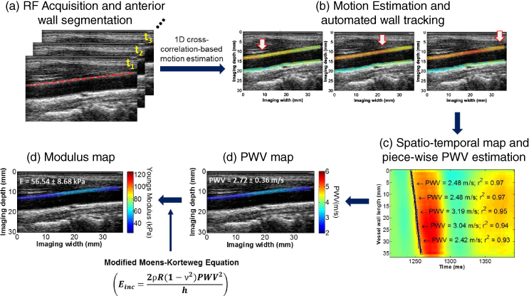
Figure 14.19 Block diagram of the pulse wave imaging (PWI) technique on a normal carotid artery in vivo. (a) RF frame sequence and ciné‐loop of RF frames. (b) PWI ciné‐loop and frames: Pulse waves induce upward wall displacement along the anterior wall. The white arrows indicate the propagation of the wavefront along the anterior wall. (c) Spatiotemporal map of the pulse wave induced displacement along the vessel length and time with a single PWV value given in the entire segment imaged. (e) PWV and (f) stiffness maps overlaid on the anterior wall of the B‐mode.
PWI is thus a localized PWV and stiffness mapping modality that is highly suitable in characterizing focal disease such as plaques before the onset of pathology (normal, thin wall) to its later stages. The parameters mapped with PWI are the PWV (Figure 14.19d), r 2 (coefficient of determination; Figure 14.19c), and compliance (Figure 14.19e), which indicate the magnitude of the velocity of the pulse wave, its uniformity of propagation, and the underlying stiffness, respectively, all of which can be mapped and used as biomarkers that are highly complementary to the ultrasound and CT scan clinical standards.
14.3.6 Methods
In order to accommodate both current clinical ultrasound practice but also ongoing methodologies developed by our group, a new PWI system was developed that optimized parameters such as beam density and frame rate. New PWI methodologies, such as those described below, are applied in phantom studies. The high frame rates facilitated by plane wave imaging allowed us to apply the following techniques that significantly enhance the quality and performance.
14.3.6.1 PWI System using Parallel Beamforming
An open‐architecture system (Vantage, Verasonics, Redmond, WA) allows for software‐based beamforming for simultaneous high frame rate and high beam density. Similar to others in the field, we have found that the performance of speckle tracking is not compromised when such systems are used, based on the advantages of differential, phase‐based measurements (as opposed to amplitude‐based approaches) [23, 32]. The acoustic exposure is on the same level as that of a standard ultrasound scanner. We have implemented such a sequence [32] that excites the transducer elements with specific delays, allowing a large field of view and then uses the delay‐and‐sum method to reconstruct the RF signals from the channel data. The associated frame rate is only limited by the depth and speed of sound. As a result, the system can obtain up to 8333 fps. Both conventional (with lower beam density to increase the frame rate) and parallel beamforming sequences are used with the same system for the purpose of this study. Because of the parallel beamforming used, the highest beam density (128 beams) and frame rate (up to 8333 fps) in PWI can simultaneously be achieved. The transducers to be used are the 128‐element linear array at a center frequency of 5.5 MHz (L7‐4 (4–7 MHz)) and the 128‐element linear array at a center frequency of 17.5 MHz (L22‐15 (15–22 MHz)) for higher spatial resolution allowing us to characterize composition and determine vulnerable plaques. We will determine the effect of lower spatial resolution and SNR associated with plane wave imaging on PWV and stiffness estimates with PWI.
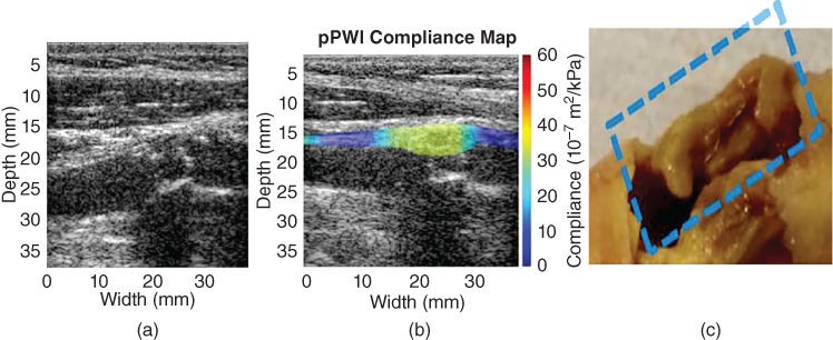
Figure 14.20 PWI in a vulnerable plaque with a fibrous cap (male, age 75). (a) Ultrasound B‐mode image only of the detected plaque. (b) PWI: B‐mode with overlaid PWI compliance map. (c) Gross pathology of the plaque with lipid core following endarterectomy. The B‐mode in part (a) provides information on the level of stenosis but not the stiffness of the plaque, like PWI in part (b). PWI was capable of mapping plaque stiffness across its thickness to identify a mostly lipid plaque (low stiffness, i.e. high compliance) confirmed by (c) pathology [138].
- Automated diameter and wall thickness algorithms have also been implemented, similar to the segmentation and tracking methods our group has already developed [27].
- PWV mapping – our fast 1D normalized cross‐correlation method is applied on the consecutively acquired RF signals to estimate the normalized wall displacement (Figure 14.19), as in our previously published studies [27, 28]. In order to obtain the regional PWV, all of the 50% upstroke points of the spatio‐temporal plots are divided into overlapping segments. 50% upstroke was determined to yield highest SNR for PWV estimation in both human aortas and carotids [130]. Fixed regression windows have been used thus far to perform linear regression for PWV estimation, especially due to the low beam density afforded by conventional beamforming techniques. A piecewise, linear regression fit has thus been developed. Sub‐regional PWVs are estimated within 2–4 mm segments along the length of the arterial wall and estimates the regional stiffness using the methodology described previously. Instead of single values for the entire vessel, this method provides maps of PWV along the entire wall imaged (Figure 14.19) but also within the plaque itself (Figure 14.20).
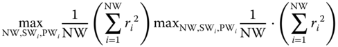
- Automated PWV estimation – a dynamic programming algorithm is implemented to automatically select the size, location, and number of windows according to a mean r
2 optimization routine with criteria based on the performance of the resulting linear regression. More specifically, the windows are appropriately selected to satisfy the maximization criterion:(14.5)where NW is the number of windows used to model the stiffness of the imaged arterial wall, SW i is the size of the i‐th window (namely the number of markers that it contains). and PW i is its position (namely the number of the starting marker).
- Stiffness/compliance mapping – the 1D system of the coupled governing pulse wave propagation is(14.6)

and
(14.7)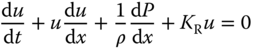
where u is the fluid velocity, P is the pressure, A is the cross‐sectional area,
 the fluid density, and
  is the resistance per unit length. The relationship between the PWV and vessel stiffness is derived by assuming a pressure–area relationship. Commonly, a thin‐walled cylindrical elastic vessel is assumed, so that the wall displacement(14.8)
for a pressure increment
 in a vessel of Young's modulus E, Poisson's ratio v, radius r, and thickness h, which gives the well‐known Moens‐Korteweg equation. In this study of carotid plaques, cylindrical geometry cannot be reasonably assumed, so we use a generalized linear pressure–area relationship, which is valid for non‐circular cross‐sections(14.9)
The compliance,
 , is related to the PWV through the Bramwell‐Hill equation 131, 132], i.e.(14.10)
and can be related to the effective Young's modulus as follows
(14.11)
that shows that compliance and stiffness are inversely proportional for a given geometry [133]. As a result, as a first approximation, the longitudinal distribution of
 can be computed by a regional PWV estimation map without homogeneity or symmetry assumptions (Figure 14.19e).
14.3.6.2 Coherent Compounding
A coherent compounding technique can be applied to determine an increase in SNR when parallel beamforming is applied. Plane waves are electronically steered and transmitted 1‐, 3‐, 5‐, 9‐ and 12‐plane‐waves and the resulting RF frames are combined into a compounded image [134]. The received radiofrequency (RF) frames are reconstructed by applying a delay‐and‐sum method on GPU‐based parallel computing to accelerate reconstruction processing [32]. In preliminary studies, we have found that compounding in human carotids in vivo decreases the frame rate from 8333 fps to 2273 fps, which remains sufficiently high for PWI (Figure 14.21) while SNR increases by 5‐fold using the framework described here (Figure 14.21a).
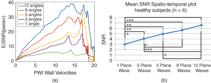
Figure 14.21 E(SNRd|δ) increase with number of angles in coherent compounding in (a) phantoms and (b) in vivo humans.
14.3.6.3 Flow Measurement
A 2D autocorrelation method is utilized [135] to generate color Doppler images (Figure 14.22a). A wall filter consisting of an FIR high‐pass filter is used to only retain the blood velocities that are fused with the corresponding PWI frames. This allows us to determine the effect of the blood pressure wave on the pulse wave propagation along the wall imaged on the PWI images as well as infer about the wall viscoelasticity (Figure 14.22b).

Figure 14.22 (a) PWI frames with Doppler flow; (b) pressure/displacement curves revealing the phase lag amount and thus viscoelasticity of the vessel (phantom). The dark curve denotes the pressure, the lighter the cumulative displacement, and the last curve shows these two overlaid.
14.3.6.4 3D PWI
A 2D matrix array (Sonic Concepts, Inc., Bothell, WA) is used in this study with a total of 1024 elements (32 × 32) and a 4.5 MHz center frequency and will be used with the Verasonics Vantage system for the highest frame rate. A custom diverging beam sequence with a virtual focus placed behind the transducer face is implemented in order to interrogate the entire field of view in a single transmit sequence. Element data is acquired and reconstructed in a pixel‐wise fashion. In sections of the common carotid prior to the bifurcation, inter‐frame pulse wave induced axial displacements (not the full 3D vector) are mapped in 3D given the lower SNR in lateral and elevational displacement estimations. Bicubic Hermite interpolation is implemented to render the vessel in 3D, which provides better visualization of the complex anatomy and motion of non‐axisymmetric plaques. The frame rate is expected to similar to 2D, i.e. up to 5500 fps, and sufficient to visualize the pulse wave and estimate the PWI parameters. 3D B‐mode feasibility and strain imaging are shown in Figure 14.23 [136].

Figure 14.23 3D PWI frames with wave propagating from right to left in a human carotid in vivo on both the proximal (top) and distal (bottom) walls.
14.3.7 PWI Performance Assessment in Experimental Phantoms
In order to ensure highest quality PWI in vivo, its performance is optimized in phantoms prior to application in vivo. Parallel beamforming provides images with reduced sonographic SNR; however, this issue has been addressed with coherent compounding. This is at the cost, however, of frame rate. Thus, by varying the number of angled plane wave acquisitions this tradeoff between frame rate and image SNR can be fine tuned and adjusted to the requirements of the application. This is verified in PVA cryogel [130] and silicone [133] phantoms with preliminary results shown in Table 14.1. Carotid artery phantoms with a plaque‐mimicking inclusion are constructed from a mixture (w/w) of 87% deionized water, 10% polyvinyl alcohol (PVA) with a molecular weight of 56.140 g/mol (Sigma‐Aldrich, St. Louis, MO, USA), and 3% graphite powder with particle size < 50 µm (Merck KGaA) [137].
Table 14.1 Preliminary validation of PWV values in a PVA phantom and a silicone phantom (with soft and stiff layers). The static PWV is a mechanical testing method. PVA: poly‐vinyl alcohol.
| Material | Static PWV estimates (m/s) | PWI‐derived PWV values (m/s) |
| Phantom 1, PVA | 1.57 | 1.53 |
| Phantom 2, soft | 2.31 | 1.86 |
| Phantom 2, stiff | 2.87 | 2.86 |
A peristaltic pump (Manostat Varistaltic, Barrington, IL) operating at 2 Hz is used. The parameters to be studied for optimizing the PWI performance are: (i) frame rate; (ii) number of transmitted plane waves (coherent compounding); (iii) motion estimation rate (MER); and (iv) size of kernel in piecewise PWI (pPWI) (PWV is estimated within these kernels). A probabilistic framework has been developed by our group in order to compare the strain estimation quality between conventional and parallel beamforming [23, 32]. The signal‐to‐noise‐ratio of the displacement (SNRd) is calculated for each sequence over the phase of systole. SNRe is computed for every point in an image within a small 2D ROI (3.0 × 3.2 mm). Since both strain and SNRd are computed for each point in the vessel, a large number (>600 000) of displacement–SNRd pairs are generated for each sequence [23]. The conditional expected values of SNRd for each strain are calculated using E(SNRd|δ) curves generated for each sequence, which allows for a relatively easy comparison to be performed between different sequences for a wide range of strain values. Examples of E(SNRd|δ) curves for displacement estimation are provided in Figure 14.21a. The SNRd of both 2D PWI and 3D PWI are computed.
14.3.8 Mechanical Testing
Three types of mechanical testing are performed to validate our in vivo PWI findings. First, in order to preserve the geometry of the sample and reproduce the in vivo pre‐stretch, effect of surrounding tissue, and loading conditions, the entire sample is kept intact and inflated at static pressures (Figure 14.24). The compliance
can be measured experimentally by applying this static pressure and measuring the diameter change on the B‐mode images. The PWV can then be estimated by
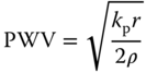
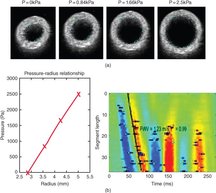
Figure 14.24 (a) Static estimation of the PWV (Eq. 14.13) from a vessel phantom compared with PWI showing the B‐mode of a phantom at different static pressures. (b) Measurements in phantom with PWI and static expansion test, respectively.
A phantom example showing good agreement between the PWV estimated through static testing and PWI is shown in Table 14.1.
14.3.9 PWI in Aortic Aneurysms and Carotid Plaques in Human Subjects In Vivo
The clinical potential of PWI to provide complementary information on the mechanical properties of vessels in order to help stage disease and inform treatment are assessed. Therefore, the underlying hypothesis of this study is that imaging the regional pulse wave propagation at high temporal resolution is sufficient to determine regional elastic vessel wall properties and thus localize and characterize focal vascular disease at its very early stages, i.e. before changes in aortic diameter or other anatomical changes may occur or become detectable. It is also hypothesized that the regional stiffness changes will unveil the regions most susceptible to wall rupture.
14.3.9.1 Abdominal Aortic Aneurysms
The clinical feasibility of PWI was evaluated in normal and aneurysmal human aortas. PWI was performed in normal (N = 15, mean age 32.5 years ± 10.2), and aneurysmal (N = 5, mean age 71.6 years ± 11.8) human subjects (Figure 14.25) [138]. The PWV of the AAA aortas was significantly higher ( p < 0.001) compared to that of the other two groups. The average r 2 in the AAA subjects was significantly lower (p < 0.001) than that in the normal subjects, very similar to what was shown in mice.
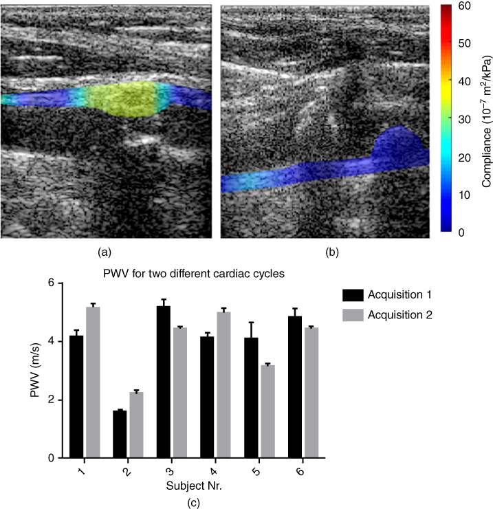
Figure 14.25 PWI compliance maps in human carotids in vivo: (a) lipid plaque (male, aged 75); (b) calcified plaque (female, aged 78); and (c) PWI reproducibility in 6 normal subjects and different acquisitions.

Figure 14.26 Preliminary compliance findings across 10 normal and 12 atherosclerotic carotids confirmed with endarterectomy and/or CT. * p < 0.05; ** p < 0.01; *** p < 0.001.
14.3.9.2 Carotid Plaques
The feasibility of PWI in normal [139] and atherosclerotic (Figure 14.20) common carotid arteries has been demonstrated in vivo. The pulse wave velocity (PWV) in eight (N = 8) normals varied between 4.0 and 5.2 m/s with high propagation uniformity (r 2 > 0.90) with excellent reproducibility (Figures 14.25 and 14.26).
Acknowledgements
The results presented here were produced by current and previous members of the Ultrasound and Elasticity Imaging Laboratory: Iason Apostolakis, PhD; Ethan Bunting, PhD; Alexandre Costet, PhD; Julien Grondin, PhD; Wei‐Ning Lee, PhD; Ronny Li, PhD; Pierre Nauleau, PhD; and Jean Provost, PhD. The studies were in part supported by grants from the National Institutes of Health: R01 EB006042, R01 HL098830, and R01 HL 114358.
References
- 1 Go, A.S., Mozaffarian, D., Roger, V.L. et al. (2014). Heart disease and stroke statistics – 2014 Update: A report From the American Heart Association. Circulation 129: e28–e292.
- 2 Haga, J.H., Beaudoin, A.J., White, J.G., and Strony, J. (1998). Quantification of the passive mechanical properties of the resting platelet. Ann. Biomed. Eng. 26: 268–277.
- 3 Bertrand, M.E., Rousseau, M.F., Lefebvre, J.M., et al. (1978). Left‐ventricular compliance in acute transmural myocardial‐infarction in man. Eur. J. Cardiol. 7: 179–193.
- 4 Neagoe, C., Kulke, M., del Monte, F., et al. (2002). Titin isoform switch in ischemic human heart disease. Circulation 106 (11): 1333–1341.
- 5 Edwards, C.H., Rankin, J. S., Mchale, P.A., et al. (1981). Effects of ischemia on left‐ventricular regional function in the conscious dog. Am. J. Physiol. 240 (3): H413–H420.
- 6 Amano, J., Thomas, J.X., Lavallee, M., et al. (1987). Effects of myocardial‐ischemia on regional function and stiffness in conscious dogs. Am. J. Physiol. 252 (1): H110–H117.
- 7 Varma, N., Eberli, F.R., and Apstein, C.S. (2000). Increased diastolic chamber stiffness during demand ischemia – Response to quick length change differentiates rigor‐activated from calcium‐activated tension. Circulation 101 (18): 2185–2192.
- 8 Varma, N., Eberl, F.R. and Apstein, C.S. (2001). Left ventricular diastolic dysfunction during demand ischemia: Rigor underlies increased stiffness without calcium‐mediated tension. Amelioration by glycolytic substrate. J. Am. Coll. Cardiol. 37 (8): 2144–2153.
- 9 Gupta, K.B., Ratcliffe, M.B., Fallert, M.A., et al. (1994). Changes in passive mechanical stiffness of myocardial tissue with aneurysm formation. Circulation 89: 2315–2326.
- 10 Holmes, J.W., Borg, T.K., and Covell, J.W. (2005). Structure and mechanics of healing myocardial infarcts. Annu. Rev. Biomed. Eng. 7: 223–253.
- 11 Konofagou, E., D'hooge, J., and Ophir, J. (2000). Cardiac elastography – A feasibility study. Proc. IEEE Ultrason. Symp. 1273–1276.
- 12 Konofagou, E.E., Harrigan, T., and Solomon, S. (2001). Assessment of regional myocardial strain using cardiac elastography: distinguishing infarcted from non‐infarcted myocardium. Proc. IEEE Ultrason. Symp. 1589–1592.
- 13 Konofagou, E.E., D'Hooge, J., and Ophir, J. (2002). Myocardial elastography – A feasibility study in vivo. Ultrasound Med. Biol. 28: 475–482.
- 14 Konofagou, E.E., Manning, W., Kissinger, K., and Solomon, S.D. (2003). Myocardial elastography – Comparison to results using MR cardiac tagging. Proc. IEEE Ultrason. Symp. 130–133.
- 15 Konofagou, E.E., Fung‐Kee‐Fung, S., Luo, J., and Pernot, M. (2006). Imaging the mechanics and electromechanics of the heart. Proc. IEEE EMBS Conf. 6648–6651.
- 16 Konofagou, E.E., Luo, J., Fujikura, K., et al. (2006). Imaging the electromechanical wave activation of the left ventricle in vivo. Proc. IEEE Ultrason. Symp. 985–988.
- 17 Konofagou, E.E., Lee, W.‐N., and Luo, J. (2008). Cardiovascular elasticity imaging. In: Biomedical Applications of Vibration and Acoustics in Imaging and Characterizations (ed. M. Fatemi, A. Al‐Jumaily). Chapter 6: 93–117. New York, NY: ASME Press.
- 18 Konofagou, E.E. and Provost, J., (2012). Electromechanical wave imaging for noninvasive mapping of the 3D electrical activation sequence in canines and humans in vivo. J. Biomech. 45(5): 856–864.
- 19 Konofagou, E. and Ophir, J. (1998). A new elastographic method for estimation and imaging of lateral displacements, lateral strains, corrected axial strains and Poisson's ratios in tissues. Ultrasound Med. Biol. 24: 1183–1199.
- 20 Provost, J., Lee, W.N., Fujikura, K., Konofagou, E.E. (2010). Electromechanical wave imaging of normal and ischemic hearts in vivo. IEEE Trans. Med. Imaging 29 (3): 625–35.
- 21 Lee, W.N., Provost, J., Fujikura, K., et al. (2011). In vivo study of myocardial elastography under graded ischemia conditions. Phys. Med. Biol. 56 (4): 1155–72.
- 22 Konofagou, E.E. and Provost, J. (2012). Electromechanical wave imaging for noninvasive mapping of the 3D electrical activation sequence in canines and humans in vivo. J. Biomech. 45 (5): 856–864.
- 23 Bunting, E., Provost, J., and Konofagou, E.E. (2014). Performance analysis of two‐dimensional cardiac strain estimation using novel sequences, different beamforming and temporal resolution in vivo. Phys. Med. Biol. 59 (22): 6841–6858.
- 24 Konofagou, E.E. (1999). Estimation and Imaging of Three‐dimensional Motion and Poisson's Ratio in Elastography. Ph.D. dissertation, University of Houston, TX.
- 25 Zervantonakis, I.K., Fung‐Kee‐Fung, S.D., Lee, W.N., and Konofagou, E.E. (2007). A novel, view‐independent method for strain mapping in myocardial elastography: eliminating angle and centroid dependence. Phys. Med. Biol. 52: 4063–4080.
- 26 Lee, W.N. and Konofagou, E.E. (2008). Angle‐independent and multi‐dimensional myocardial elastography – From theory to clinical validation. Ultrasonics 48: 563–567.
- 27 Luo, J. and Konofagou, E. (2010). A fast normalized cross‐correlation calculation method for motion estimation. IEEE Trans. Ultrason., Ferroelect., Freq. Control 57 (6): 1347–1357.
- 28 Luo J., Lee, W.‐N., and Konofagou, E.E. (2009). Fundamental performance assessment of 2‐D myocardial elastography in a phased array configuration. IEEE Trans. Ultrason., Ferroelect., Freq. Control 56 (10): 2620–2627.
- 29 Righetti, R., Ophir, J., and Ktonas, P. (2002). Axial resolution in elastography. Ultrasound Med. Biol. 28 (1): 101–113.
- 30 Lee, W.N., Ingrassia, C.M., Fung‐Kee‐Fung, S.D., et al. (2007). Theoretical quality assessment of myocardial elastography with in vivo validation. IEEE Trans. Ultrason., Ferroelect., Freq. Control 54: 2233–2245.
- 31 Kallel, F. and Ophir, J. (1997). A least‐squares strain estimator for elastography. Ultrason. Imaging 19: 195–208.
- 32 Provost, J. Thiebault, S., Luo, J. and Konofagou, E.E. (2012). Single‐heartbeat electromechanical wave imaging with optimal strain estimation using temporally‐unequispaced acquisition sequences. Phys. Med. Biol. 57 (4): 1095–1112.
- 33 Jensen, J.A. and Svendsen, N.B. (1992). Calculation of pressure fields from arbitrarily shaped, apodized, and excited ultrasound transducers. IEEE Trans. Ultrason., Ferroelect., Freq. Control 39: 262–267.
- 34 Jensen, J.A. (1996). Field: a program for simulating ultrasound systems. Paper presented at the 10th Nordic‐Baltic Conference on Biomedical Imaging. Med. Biol. Eng. Comput. 34: 1351–1353.
- 35 Luo, J. and Konofagou, E.E. (2008). High‐frame rate, full‐view myocardial elastography with automated contour tracking in murine left ventricles in vivo. IEEE Trans. Ultrason., Ferroelect., Freq. Control 55: 240–248.
- 36 Lloyd‐Jones, D., Adams, R., Carnethon, M. et al. (2009). Heart disease and stroke statistics – 2009 update: a report from the American Heart Association Statistics Committee and Stroke Statistics Subcommittee. Circulation 119 (3): e21–181.
- 37 Haïssaguerre, M., Jaïs, P., Shah, D.C., et al. (1998). Spontaneous initiation of atrial fibrillation by ectopic beats originating in the pulmonary veins. N. Engl. J. Med. 339: 659–666.
- 38 Ashikaga, H., Coppola, B.A., Hopenfeld, B., et al. (2007). Transmural dispersion of myofiber mechanics: implications for electrical heterogeneity in vivo. J. Am. Coll. Cardiol. 49: 909–916.
- 39 Cordeiro, J.M., Greene, L., Heilmann, C., et al. (2004). Transmural heterogeneity of calcium activity and mechanical function in the canine left ventricle. Am. J. Physiol. Heart Circ. Physiol. 286: H1471–1479.
- 40 Pernot, M. and Konofagou, E.E. (2005). Electromechanical imaging of the myocardium at normal and pathological states. Proc. IEEE Ultrason. Symp. 2005: 1091–1094.
- 41 Konofagou, E.E., Lee, W.‐N., and Fung‐Kee‐Fung, S.D. (2007). Angle‐independent myocardial elastography: Theoretical analysis and clinical validation. Proc. SPIE, 6513: 65130G‐1–65130G‐10.
- 42 Konofagou, E.E., Luo, J., Saluja, D., et al. (2007). Noninvasive electromechanical wave imaging and conduction velocity estimation in vivo. Proc. IEEE Ultrason. Symp. 2007: 969–972.
- 43 Konofagou, E.E., Luo, J., Saluja, D., et al. (2010). Noninvasive electromechanical wave imaging and conduction‐relevant velocity estimation in vivo. Ultrasonics 50: 208–215.
- 44 Konofagou, E.E., Lee, W.‐N., Luo, J., et al. (2011). Physiologic cardiovascular strain and intrinsic wave imaging, Annu. Rev. Biomed. Eng. 13: 477–505.
- 45 Wang, S.G., Lee, W.N., Provost, J. et al. (2008). A composite high‐frame‐rate system for clinical cardiovascular imaging. IEEE Trans. Ultrason., Ferroelect., Freq. Control 55: 2221–2233.
- 46 Provost, J., Gurev, V., Trayanova, N., and Konofagou, E.E. (2011). Mapping of cardiac electrical activation with electromechanical wave imaging: an in silico‐in vivo reciprocity study. Heart Rhythm 8 (5): 752–759.
- 47 Provost, J., Nguyen, V.T., Legrand, D., et al. (2011). Electromechanical wave imaging for arrhythmias. Phys. Med. Biol. 56 (22): L1–11.
- 48 Provost, J., Lee, W.‐N., Fujikura, K., and Konofagou E.E. (2011). Imaging the electromechanical activity of the heart in vivo, Proc. Natl. Acad. Sci. 108 (21): 8565–8570.
- 49 Gurev, V., Constantino, J., Rice, J.J., and Trayanova, N.A.. (2010). Distribution of electromechanical delay in the heart: Insights from a three‐dimensional electromechanical model. Biophys. J. 99 (3): 745–754.
- 50 Garan, H. (2008). Atypical atrial flutter. Heart Rhythm 5: 618–621.
- 51 Saoudi, N., Cosío, F., Waldo, A., et al. (2001). A classification of atrial flutter and regular atrial tachycardia according to electrophysiological mechanisms and anatomical bases. A statement from a Joint Expert Group from The Working Group of Arrhythmias of the European Society of Cardiology and the North American Society of Pacing and Electrophysiology. Eur. Heart J. 22: 1162–1182.
- 52 Bochoeyer, A., Yang, Y., Cheng, J., et al. (2003). Surface electrocardiographic characteristics of right and left atrial flutter. Circulation 108: 60–66.
- 53 Nash, M.P. and Pullan, A.J. (2005). Challenges facing validation of noninvasive electrical imaging of the heart. Ann. Noninvasive Electrocardiol. 10: 73–82.
- 54 Chattipakorn, N. and Ideker, R.E. (2003). The vortex at the apex of the left ventricle: A new twist to the story of the electrical induction of rotors? J. Cardiovasc. Electrophysiol. 14: 303–305.
- 55 Durrer, D., Van Dam, R.T., Freud, G.E., et al. (1970). Total excitation of the isolated human heart. Circulation 41: 899–912.
- 56 Sutherland, D.R., Ni, Q., MacLeod, R.S., et al. (2008). Experimental measures of ventricular activation and synchrony. Pacing Clin. Electrophysiol. 31: 1560–1570.
- 57 Kay, M.W., Amison, P.M., and Rogers, J.M. (2004). Three‐dimensional surface reconstruction and panoramic optical mapping of large hearts. IEEE Trans. Biomed. Eng. 51: 1219–1229.
- 58 Qu, F., Ripplinger, C.M., Nikolski, V.P., et al. (2007). Three‐dimensional panoramic imaging of cardiac arrhythmias in rabbit heart. J. Biomed. Opt. 12: 044019.
- 59 Ripplinger, C.M., Lou, Q., Li, W., et al. (2009). Panoramic imaging reveals basic mechanisms of induction and termination of ventricular tachycardia in rabbit heart with chronic infarction: implications for low‐voltage cardioversion. Heart Rhythm 6: 87–97.
- 60 Hooks, D.A., LeGrice, I.J., Harvey, J.D., and Smaill, B.H. (2001). Intramural multisite recording of transmembrane potential in the heart. Biophys. J. 81: 2671–2680.
- 61 Hillman, E.M.C., Bernus, O., Pease, E., et al. (2007). Depth‐resolved optical imaging of transmural electrical propagation in perfused heart. Opt. Express 15: 17827–17841.
- 62 Kong, W., Ideker, R.E., and Fast, V.G. (2009). Transmural optical measurements of V m dynamics during long‐duration ventricular fibrillation in canine hearts. Heart Rhythm 6: 796–802.
- 63 Zhang, X., Ramachandra, I., Liu, Z., et al. (2005). Noninvasive three‐dimensional electrocardiographic imaging of ventricular activation sequence. Am. J. Physiol. Heart Circ. Physiol. 289: H2724–32.
- 64 Ramanathan, C., Ghanem, R.N., Jia, P., et al. (2004). Noninvasive electrocardiographic imaging for cardiac electrophysiology and arrhythmia. Nat. Med. 10: 422–428.
- 65 Ramanathan, C., Jia, P., Ghanem, R., et al. (2006). Activation and repolarization of the normal human heart under complete physiological conditions. Proc. Natl. Acad. Sci. 103: 6309 –6314.
- 66 Schilling, R.J., Peters, N.S., and Davies, W. (1998). Simultaneous endocardial mapping in the human left ventricle using a noncontact catheter – Comparison of contact and reconstructed electrograms during sinus rhythm. Circulation 98: 887–898.
- 67 Tai, C.‐T., Liu, T.‐Y., Lee, P.‐C., et al. (2004). Non‐contact mapping to guide radiofrequency ablation of atypical right atrial flutter. J. Am. Coll. Cardiol. 44: 1080–1086.
- 68 Taccardi, B., Arisi, G., Macchi, E., et al. (1987). A new intracavitary probe for detecting the site of origin of ectopic ventricular beats during one cardiac cycle. Circulation 75: 272–281.
- 69 Wang, Y., Schuessler, R.B., Damiano, R.J., et al. (2007). Noninvasive electrocardiographic imaging (ECGI) of scar‐related atypical atrial flutter. Heart Rhythm 4: 1565–1567.
- 70 Belgacem, F.B. (2007). Why is the Cauchy problem severely ill‐posed? Inverse Probl. 23: 823–836.
- 71 Lux, R.L. (2008). Noninvasive assessment of cardiac electrophysiology for predicting arrhythmogenic risk: are we getting closer? Circulation 118: 899–900.
- 72 Olshansky, B. (2011). Electrocardiographic imaging: Back to the drawing board? Heart Rhythm 8: 700–701.
- 73 Badke, F.R., Boinay, P., and Covell, J.W. (1980). Effects of ventricular pacing on regional left ventricular performance in the dog. Am. J. Physiol. Heart Circ. Physiol. 238: H858–867.
- 74 Wyman, B.T., Hunter, W.C., Prinzen, F.W., and McVeigh, E.R. (1999). Mapping propagation of mechanical activation in the paced heart with MRI tagging. Am. J. Physiol. Heart Circ. Physiol. 276: H881–891.
- 75 Provost, J., Gambhir, A., Vest, J., et al. (2013). A clinical feasibility study of atrial and ventricular electromechanical wave imaging. Heart Rhythm 10 (6): 856–862.
- 76 Provost, J., Papadacci, C., Arango, J., et al. (2014). 3D ultrafast ultrasound imaging. Phys. Med. Biol. 59 (19): L1–L13.
- 77 Provost, J., Costet, A., Wan, E., et al. (2015). Assessing the atrial electromechanical coupling during atrial focal tachycardia, flutter, and fibrillation using electromechanical wave imaging in humans, Comput. Biol. Med. 65: 161–167.
- 78 Costet, A., Provost, J., Gambhir, A., et al. (2014). Electromechanical wave imaging of biologically and electrically paced canine hearts in vivo. Ultrasound Med. Biol. 40 (1): 177–187.
- 79 Costet, A., Bunting, E., Grondin, J., et al. (2015). Atrial electromechanical cycle length mapping in paced canine hearts in vivo. IEEE Trans. Ultrason., Ferroelect., Freq. Control 62 (7): 1277–1287.
- 80 Luo, J. and Konofagou, E.E. (2008). High‐frame rate, full‐view myocardial elastography with automated contour tracking in murine left ventricles in vivo. IEEE Trans. Ultrason., Ferroelect., Freq. Control 55: 240–248.
- 81 Baghani, A., Brant, A., Salcudean, S., and Rohling, R. (2010). A high‐frame‐rate ultrasound system for the study of tissue motions. IEEE Trans. Ultrason., Ferroelect., Freq. Control 57: 1535–1547.
- 82 Varghese, T. and Ophir, J. (1997). A theoretical framework for performance characterization of elastography: the strain filter. IEEE Trans. Ultrason., Ferroelect., Freq. Control 44: 164–172.
- 83 Weinstein, E. and Weiss, A. (1984). Fundamental limitations in passive time‐delay estimation – Part II: Wide‐band systems. IEEE Trans. Acoust., Speech, Signal Process. 32: 1064–1078.
- 84 Meunier, J. and Bertrand, M. (1995). Ultrasonic texture motion analysis: theory and simulation. IEEE Trans. Med. Imaging 14: 293–300.
- 85 Chen, J., Mandapati, R., Berenfeld, O., et al. (2000). High‐frequency periodic sources underlie ventricular fibrillation in the isolated rabbit heart. Circ. Res. 86: 86–93.
- 86 Ciaccio, E., Biviano, A.B., Whang, W., et al. (2011) A new transform for the analysis of complex fractionated atrial electrograms. BioMed. Eng. OnLine 10: 35.
- 87 Nauleau, P., Melki, L., Wan, E., Konofagou, E. (2017). A 3‐D rendering algorithm for electromechanical wave imaging of a beating heart. Med. Phys. 44 (9): 4766–4772.
- 88 Rosamond, W., Flegal, K., Friday, G., et al. (2007). American Heart Association Statistics C, Stroke Statistics S. Heart disease and stroke statistics – 2007 update: a report from the American Heart Association Statistics Committee and Stroke Statistics Subcommittee. Circulation 115 (5): e69–171.
- 89 Makris, G.C., Nicolaides, A.N., Xu, X.Y., Geroulakos, G. (2010). Introduction to the biomechanics of carotid plaque pathogenesis and rupture: review of the clinical evidence. Br. J. Radiol. 83 (993): 729–35.
- 90 Timsit, S.G., Sacco, R.L., Mohr, J.P., et al. (1992). Early clinical differentiation of cerebral infarction from severe atherosclerotic stenosis and cardioembolism. Stroke 23 (4): 486–491.
- 91 Maurice, R.L., Fromageau, J., Brusseau, E., et al. (2007). On the potential of the Lagrangian estimator for endovascular ultrasound elastography: in vivo human coronary artery study. Ultrasound Med. Biol. 33(8): 1199–205.
- 92 Naghavi, M., Libby, P., Falk, E., et al. (2003). From vulnerable plaque to vulnerable patient: a call for new definitions and risk assessment strategies: Part I. Circulation 108 (14): 1664–72.
- 93 Huang, H., Virmani, R., Younis, H., et al. (2001). The impact of calcification on the biomechanical stability of atherosclerotic plaques. Circulation 103 (8): 1051–1056.
- 94 Loree, H.M., Kamm, R.D., Stringfellow, R.G., Lee, R.T. (1992). Effects of fibrous cap thickness on peak circumferential stress in model atherosclerotic vessels. Circulation Res. 71 (4): 850–858.
- 95 Burke, A.P., Farb, A., Malcom, G.T., et al. (1997). Coronary risk factors and plaque morphology in men with coronary disease who died suddenly. N. Engl. J. Med. 336 (18): 1276–1282.
- 96 Virmani, R., Burke, A.P., Kolodgie, F.D., Farb, A. (2003). Pathology of the thin‐cap fibroatheroma: a type of vulnerable plaque. J. Interv. Cardiol. Electrophysiol. 16 (3): 267–272.
- 97 Redgrave, J.N., Gallagher, P., Lovett, J.K., Rothwell, P.M. (2008). Critical cap thickness and rupture in symptomatic carotid plaques: the Oxford plaque study. Stroke 39 (6): 1722–1729.
- 98 Cheng, G.C., Loree, H.M., Kamm, R.D., et al. (1993). Distribution of circumferential stress in ruptured and stable atherosclerotic lesions. A structural analysis with histopathological correlation. Circulation 87 (4): 1179–1187.
- 99 Cardoso, L. and Weinbaum, S. (2014). Changing views of the biomechanics of vulnerable plaque rupture: a review. Ann. Biomed. Eng. 42 (2): 415–431.
- 100 Lee, R.T., Richardson, S.G., Loree, H.M., et al. (1992). Prediction of mechanical properties of human atherosclerotic tissue by high‐frequency intravascular ultrasound imaging. An in vitro study. Arterioscler. Thromb. 12 (1): 1–5.
- 101 Lehmann, E.D., Hopkins, K.D., Jones, R.L., et al. (1995). Aortic distensibility in patients with cerebrovascular disease. Clin. Sci. 89 (3): 247–253.
- 102 Hirai, T., Sasayama, S., Kawasaki, T., Yagi, S. (1989). Stiffness of systemic arteries in patients with myocardial infarction. A noninvasive method to predict severity of coronary atherosclerosis. Circulation 80 (1): 78–86.
- 103 Gatzka, C.D., Cameron, J.D., Kingwell, B.A., Dart, A.M. (1998). Relation between coronary artery disease, aortic stiffness, and left ventricular structure in a population sample. Hypertension 32 (3): 575–578.
- 104 Giannattasio, C., Failla, M., Emanuelli, G., et al. (2001). Local effects of atherosclerotic plaque on arterial distensibility. Hypertension 38 (5): 1177–1180.
- 105 Raghavan, M.L., Vorp, D.A., Federle, M.P., et al. (2000). Wall stress distribution on three‐dimensionally reconstructed models of human abdominal aortic aneurysm. J. Vasc. Surg. 31 (4): 760–769.
- 106 Canton, G., Hippe, D.S., Sun, J., et al. (2012). Characterization of distensibility, plaque burden, and composition of the atherosclerotic carotid artery using magnetic resonance imaging. Med. Phys. 39 (10): 6247–6253.
- 107 Ouriel, K., Green, R.M., Donayre, C., et al. (1992). An evaluation of new methods of expressing aortic aneurysm size: relationship to rupture. J. Vasc. Surg. 15 (1): 12–18.
- 108 Bengtsson, H., Sonesson, B., Bergqvist, D. (1996). Incidence and prevalence of abdominal aortic aneurysms, estimated by necropsy studies and population screening by ultrasound. Ann. NY Acad. Sci. 800: 1–24.
- 109 Patel, M.I., Hardman, D.T., Fisher, C.M., Appleberg, M. (1995). Current views on the pathogenesis of abdominal aortic aneurysms. J. Am. Coll. Surg. 181 (4): 371–382.
- 110 Darling, R.C., Messina, C.R., Brewster, D.C., Ottinger, L.W. (1977). Autopsy study of unoperated abdominal aortic aneurysms. The case for early resection. Circulation 56 (3 Suppl): II161–164.
- 111 Wain, R.A., Marin, M.L., Ohki, T. et al. (1998). Endoleaks after endovascular graft treatment of aortic aneurysms: classification, risk factors, and outcome. J. Vasc. Surg. 27 (1): 69–78, discussion 78–80.
- 112 Turnipseed, W.D., Carr, S.C., Tefera, G., et al. (2001). Minimal incision aortic surgery. J. Vasc. Surg. 34 (1): 47–53.
- 113 Velazquez, O.C., Larson, R.A., Baum, R.A., et al. (2001). Gender‐related differences in infrarenal aortic aneurysm morphologic features: issues relevant to Ancure and Talent endografts. J. Vasc. Surg. 33 (2 Suppl): S77–84.
- 114 Gabrielli, L., Baudo, A., Molinari, A., Domanin, M. (2004). Early complications in endovascular treatment of abdominal aortic aneurysm. Acta Chirurgica Belgica 104 (5): 519–526.
- 115 Ghansah, J.N. and Murphy, J.T. (2004). Complications of major aortic and lower extremity vascular surgery. Semin. Cardiothorac. Vasc. Anesth. 8 (4): 335–361.
- 116 Dillavou, E.D., Muluk, S.C., Makaroun, M.S. (2006). A decade of change in abdominal aortic aneurysm repair in the United States: Have we improved outcomes equally between men and women? J. Vasc. Surg. 43 (2): 230–238; discussion 238.
- 117 Brewster, D.C., Cronenwett, J.L., Hallett, J.W., Jr., et al. (2003). Joint Council of the American Association for Vascular Surgery and Society for Vascular Surgery. Guidelines for the treatment of abdominal aortic aneurysms. Report of a subcommittee of the Joint Council of the American Association for Vascular Surgery and Society for Vascular Surgery. J. Vasc. Surg. 37 (5): 1106–1117.
- 118 Choksy, S.A., Wilmink, A.B.M., and Quick, C.R. (1999). Ruptured abdominal aortic aneurysm in the Huntingdon district: a 10‐year experience. Ann. R. Coll. Surg. Engl. 81: 27–31.
- 119 Hall, A.J., Busse, E.F.G., McCarville, D.J. and Burgess, J.J. (2000). Aortic wall tension as a predictive factor for abdominal aortic aneurysm rupture: Improving the selection of patients for abdominal aortic aneurysm repair. Ann. Vasc. Surg. 14: 152–157.
- 120 Vorp, D.A. (2007). Biomechanics of abdominal aortic aneurysm. J. Biomech. 40: 1887–1902.
- 121 Darling, R.C., Messina, C.R., Brewster, D.C. and Ottinger, L.W. (1977). Autopsy study of unoperated abdominal aortic‐aneurysms – case for early resection. Circulation 56: 161–164.
- 122 Hartley, C.J., Taffet, G.E., Michael, L.H., et al. (1997). Noninvasive determination of pulse‐wave velocity in mice. Am. J. Physiol. 42: H494–H500.
- 123 Brands, P.J., Hoeks, A.P.G., Ledoux, L.A.F., and Reneman, R.S. (1997). A radio frequency domain complex cross‐correlation model to estimate blood flow velocity and tissue motion by means of ultrasound. Ultrasound Med. Biol. 23: 911–920.
- 124 Meinders, J.M., Kornet, L., Brands, P.J. and Hoeks, A.P.G. (2001). Assessment of local pulse wave velocity in arteries using 2D distension waveforms. Ultrason. Imaging 23: 199–215.
- 125 Eriksson, A., Greiff, E., Loupas, T., et al. (2002). Arterial pulse wave velocity with tissue Doppler imaging. Ultrasound Med. Biol. 28: 571–580.
- 126 Rabben, S.I., Stergiopulos, N., Hellevik, L.R., et al. (2002). An ultrasound‐based method for determining pulse‐wave velocity in the carotid artery. Eur. Heart J. 23: 611–611.
- 127 Hermeling, E., Reesink, K.D., Reneman, R.S., and Hoeks, A.P.G. (2007). Measurement of local pulse wave velocity: Effects of signal processing on precision. Ultrasound Med. Biol. 33: 774–781.
- 128 Hoctor, R.T., Dentinger, A.M., and Thomenius, K.E. (2007). Array signal processing for local arterial pulse wave velocity measurement using ultrasound. IEEE Trans. Ultrason., Ferroelect., Freq. Control 54: 1018–1027.
- 129 Mancia, G., de Backer G., Dominiczak A., et al. (2007). 2007 Guidelines for the management of arterial hypertension: The task force for the management of arterial hypertension of the European Society of Hypertension (ESH) and of the European Society of Cardiology (ESC). J. Hypertens. 25 (6): 1105–1187.
- 130 Li, R.X., Qaqish, W.W., and Konofagou, E.E. (2015). Performance assessment of pulse wave imaging using conventional ultrasound in canine aortas ex vivo and normal human arteries in vivo. Artery Res. 11: 19–28.
- 131 Westenberg, J.J., van Poelgeest, E.P., Steendijk, P, et al. (2012). Bramwell‐Hill modeling for local aortic pulse wave velocity estimation: a validation study with velocity‐encoded cardiovascular magnetic resonance and invasive pressure assessment. J. Cardiovasc. Magn. Reson. 14: 2.
- 132 Asmar, R., Benetos, A., Topouchian, J., et al. (1995). Assessment of arterial distensibility by automatic pulse wave velocity measurement. Validation and clinical application studies. Hypertension 26 (3): 485–490.
- 133 McGarry, M., Li, R., Apostolakis, I., et al. (2016). An inverse approach to determining spatially varying arterial compliance using ultrasound imaging. Phys. Med. Biol. 61 (15): 5486–5507.
- 134 Apostolakis, I.‐Z., Nandlall, S.D., Konofagou, E.E. (2016). Adaptive stiffness mapping in murine atherosclerotic and aneurysmal aortas using pulse wave imaging (PWI) in vivo. IEEE Trans. Med. Imaging 35 (1): 13–28.
- 135 Waksman, R., Serruys, P.W., and Schaar, J. (2007). Handbook of the Vulnerable Plaque. CRC Press.
- 136 Apostolakis, I.Z., Nauleau, P., Papadacci, C., et al. (2017). Feasibility and validation of 4‐D pulse wave imaging in phantoms and in vivo. IEEE Trans. Ultrason., Ferroelect., Freq. Control 64 (9): 1305–1317.
- 137 Widman, E., Maksuti, E., Larsson, D., et al. (2015). Shear wave elastography plaque characterization with mechanical testing validation: a phantom study. Phys. Med. Biol. 60 (8): 3151–3174.
- 138 Li, R.X., Luo, J., Balaram, S.K., et al. (2013). Pulse wave imaging in normal, hypertensive and aneurysmal human aortas in vivo: a feasibility study. Phys. Med. Biol. 58 (13): 4549–4562.
- 139 Luo, J., Li, R.X., Konofagou, E.E. (2012). Pulse wave imaging of the human carotid artery: an in vivo feasibility study. IEEE Trans. Ultrason., Ferroelect., Freq. Control 59 (1): 174–181.