
15
Dynamic Elasticity Imaging
Kevin J. Parker
Department of Electrical and Computer Engineering, University of Rochester, Rochester, NY, USA
15.1 Vibration Amplitude Sonoelastography: Early Results
Vibration amplitude sonoelastography entails the application of a continuous low‐frequency vibration (40–1000 Hz) to excite internal shear waves within the tissue of interest [1, 2]. A disruption in the normal vibration patterns will result if a stiff inhomogeneity is present in soft tissue surroundings. A real‐time vibration image can be created by Doppler detection algorithms. Modal patterns can be created in certain organs with regular boundaries. The shear wave speed of sound in the tissue of these organs can be ascertained with the information revealed by these patterns [3].
Figure 15.1 reproduces the first vibration‐amplitude sonoelastography image [1, 2], which marked the emergence of elastography imaging from the previous studies of tissue motion. The vibration within a sponge and saline phantom containing a harder area (the dark region) is depicted by this low resolution image. Range‐gated Doppler was used to calculate the vibration amplitude of the interior of the phantom as it was vibrated from below. By 1990, a modified color Doppler instrument was used by the University of Rochester group to create real‐time vibration‐amplitude sonoelastography images. In these images, vibration above a certain threshold (in the 2 µm range) produced a saturated color (Figure 15.2).

Figure 15.1 Original imaging data and schematic of the first known image of relative stiffness, derived from Doppler data in a phantom with applied vibration. The original image was published in 1987 and 1988 and marks the emergence of elastographic imaging.
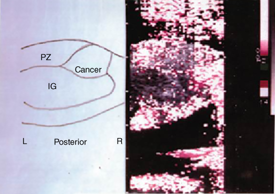
Figure 15.2 A representative first‐generation image of vibration sonoelastography, circa 1990. Doppler spectral variance is employed as an estimator of vibration in the 1–10 µm range and displayed over the B‐scan images. No color implies low vibrations below threshold. Shown is the fill‐in of vibration within a whole prostate, with a growing cancerous region indicated by the deficit of color within the peripheral zone. Source: courtesy of Dr. R. M. Lerner; Anastasio and La Riviere [4], Figure 12.4, p. 186; reproduced with permission from Taylor and Francis Group.
Measurements of tissue elastic constants, finite‐element modeling results, and phantom and ex vivo tissue sonoelastography were later reported [5–7]. Thus, by the end of 1990, the working elements of vibration elastography (sonoelastography and sonoelasticity were other names used at the time) were in place, including real‐time imaging techniques and stress‐strain analysis of tissues such as prostate, with finite‐element models and experimental images demonstrating conclusively that small regions of elevated Young's modulus could be imaged and detected using conventional Doppler‐imaging scanners.
15.2 Sonoelastic Theory
Along with the useful finite‐element approach of Lerner et al. [5] and Parker et al. [7], there were important theoretical questions to be answered by analytical or numerical techniques. How did vibration fields behave in the presence of elastic inhomogeneities? What is the image contrast of lesions in a vibration field, and how does the contrast depend on the choice of parameters? How do we optimally detect sinusoidal vibration patterns and image them using Doppler or related techniques? These important issues were addressed in a series of papers through the 1990s. One foundational result was published in 1992 under the title: “Sonoelasticity of Organs, Shear Waves Ring a Bell” [3]. This paper demonstrated experimental proofs that vibrational eigenmodes could in fact be created in whole organs, including the liver and kidneys, where extended surfaces create reflections of sinusoidal steady‐state shear waves. Lesions would produce a localized perturbation of the eigenmode pattern, and the background Young's modulus could be calculated from the patterns at discrete eigenfrequencies. Thus, both quantitative and relative imaging contrast detection tasks could be completed with vibration elastography in a clinical setting, in vivo, by 1992. A later review of eigenmodes and a strategy for using multiple frequencies simultaneously (called “chords”) was given in Taylor et al. [8].
Furthermore, a vibration‐amplitude analytical model was created [9, 10]. This model used a sonoelastic Born approximation to solve the wave equations in an inhomogeneous, isotropic medium. The total shear wave field inside the medium can be expressed as
where ![]() is the homogeneous or incident field, and
is the homogeneous or incident field, and ![]() is the field scattered by the inhomogeneity. They satisfy, respectively
is the field scattered by the inhomogeneity. They satisfy, respectively
where ![]() is a function of the properties of inhomogeneity and
is a function of the properties of inhomogeneity and ![]() is the wavenumber of shear wave propagation at a frequency
is the wavenumber of shear wave propagation at a frequency ![]() . The theory accurately describes how a hard or soft lesion appear as disturbances in a vibration pattern. Figure 15.3 summarizes the theoretical and experimental trends.
. The theory accurately describes how a hard or soft lesion appear as disturbances in a vibration pattern. Figure 15.3 summarizes the theoretical and experimental trends.

Figure 15.3 Theoretical results of the contrast of vibration sonoelastography for soft or hard lesions in a background medium. The image contrast increases with both increasing frequency and with increasing size of the lesion.
Signal processing estimators were also developed in the study of vibration amplitude sonoelastography. Huang et al. suggested a method to estimate a quantity denoted ![]() , which is proportional to the vibration amplitude of the target, from the spectral spread [11]. They found a simple correlation between
, which is proportional to the vibration amplitude of the target, from the spectral spread [11]. They found a simple correlation between ![]() and the Doppler spectral spread
and the Doppler spectral spread ![]()
where ![]() is the vibration frequency of the vibrating target. This is an uncomplicated and very useful property of the Bessel Doppler function. The effect of noise, sampling, and nonlinearity on the estimation was also considered. In their later work, they studied real‐time estimators of vibration amplitude, phase, and frequency that could be used for a variety of vibration sonoelastography techniques [12].
is the vibration frequency of the vibrating target. This is an uncomplicated and very useful property of the Bessel Doppler function. The effect of noise, sampling, and nonlinearity on the estimation was also considered. In their later work, they studied real‐time estimators of vibration amplitude, phase, and frequency that could be used for a variety of vibration sonoelastography techniques [12].
Finally, an overall theoretical approach that places vibration sonoelastography on a biomechanical spectrum with other techniques including compression elastography, magnetic resonance elastography (MRE), and the use of impulsive radiation force excitations, is found in “A Unified View of Imaging the Elastic Properties of Tissues” [13]. This perspective is highlighted in Chapter of this book.
15.3 Vibration Phase Gradient Sonoelastography
In parallel to the early work at the University of Rochester, a vibration phase gradient approach to sonoelastography was developed by Sato and collaborators at the University of Tokyo [14]. They mapped the amplitude and the phase of low frequency wave propagation inside tissue. From this mapping, they were able to derive wave‐propagation velocity and dispersion properties, which are directly linked to the elastic and viscous characteristics of tissue.
The phase‐modulated (PM) Doppler spectrum of the signal returned from sinusoidally oscillating objects approximates that of a pure‐tone frequency modulation (FM) process, as given in Eq. (15.2). This similarity indicates that the tissue vibration amplitude and phase of tissue motion may be estimated from the ratios of adjacent harmonics. The amplitude ratio between contiguous Bessel bands of the spectral signal is
where ![]() is the amplitude at the i‐th harmonic,
is the amplitude at the i‐th harmonic, ![]() is the unknown amplitude of vibration in the tissue, and
is the unknown amplitude of vibration in the tissue, and ![]() is an i‐th order Bessel function.
is an i‐th order Bessel function. ![]() can be estimated from the experimental data if
can be estimated from the experimental data if ![]() is calculated as a function of
is calculated as a function of ![]() beforehand. The phase of the vibration was calculated from the quadrature signals.
beforehand. The phase of the vibration was calculated from the quadrature signals.
The display of wave propagation as a moving image is permitted by constructing phase and amplitude maps (Figure 15.4) as a function of time. The use of a minimum squared error algorithm to estimate the direction of wave propagation and to calculate phase and amplitude gradients in this direction allows images of amplitude and phase to be computed offline. By assuming that the shear viscosity effect is negligible at low frequencies, Sato's group obtained preliminary in vivo results [14].
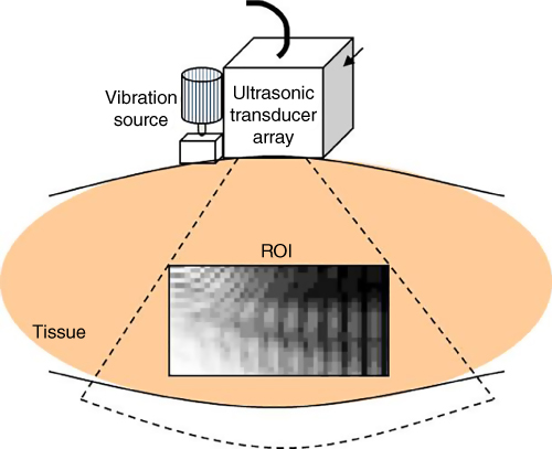
Figure 15.4 A depiction of the system developed by Prof. Sato and colleagues at the University of Tokyo, including external vibration and an imaging array with signal processing for estimating the phase of the vibration in tissue. The rate of change of phase can be estimated to yield tissue hardness.
Sato's technique was used and refined by Levinson [15], who developed a more general model of tissue viscoelasticity and a linear recursive filtering algorithm based on cubic B‐spline functions. Levinson took the Fourier transform of the wave equation and derived the frequency‐domain displacement equation for a linear, homogeneous, isotropic viscoelastic material. From this, equations that relate the shear modulus of elasticity and viscosity to the wave number and the attenuation coefficient of the wave can be derived.
Levinson et al. [15] conducted a series of experiments on the quadriceps muscle group in human thighs. It was assumed that shear waves predominate and that viscosity at low frequencies is negligible. Phase gradient images of the subjects' thighs under conditions of active muscle contraction enabled the calculation of Young's modulus of elasticity. The tension applied to the muscle was controlled using a pulley device. The measured vibration propagation speed and the calculated values of Young's modulus increased with the increasing degrees of contraction needed to counteract the applied load.
15.4 Crawling Waves
A fascinating extension of vibration sonoelastography is the use of an interference pattern formed by two parallel shear wave sources. The interference patterns reveal the underlying local elastic modulus of the tissue. The term “crawling waves” comes from the useful fact that by implementing a slight frequency difference, typically on the order of 0.1 Hz, between the two parallel sources, the interference pattern will move across the imaging plane at a speed controlled by the sources [16]. Thus, the crawling waves are readily visualized by conventional Doppler imaging scanners at typical Doppler frame rates; there is no need for ultrafast scanning. Other advantages of crawling waves include: (1) the region of interest excited between the two sources is large; (2) most of the energy in the crawling waves is aligned in the Doppler (axial) direction; and (3) a number of analysis or estimation schemes can be applied in a straightforward manner to derive the quantitative estimate of local shear wave velocity and Young's modulus. Crawling waves can also be implemented by a number of techniques including mechanical line sources, surface applicators, or radiation force excitations of parallel beams.
The use of crawling waves was first described in 2004 by Wu et al. at the University of Rochester [16]. It was shown that crawling waves could be used to accurately derive the Young's modulus of materials and to delineate stiff inclusions [17–20]. Estimators of shear wave speed and Young's modulus and the shear wave attenuation are derived by Hoyt et al. [21–23] and McLaughlin et al. [24].
Implementation into scanning probes can be accomplished by utilizing radiation force excitation along parallel beams [25–27], or by utilizing a pair of miniature vibration sources [28].
15.5 Clinical Results
The initial applications of amplitude sonoelastography were to characterize average tissue properties using eigenmode information [3, 29] and to identify stiff lesions by the amplitude contrast effect. In particular, the demonstration of improved detectability of prostate cancer was published in Radiology in 1995 [30]. This work was then adapted to in vivo and 3D studies of the prostate [8, 19, 31–34], and it was demonstrated that the sensitivity and specificity of prostate cancer detection could be markedly improved using sonoelasticity. Separately, it was shown that the definition and volumetric measurement of thermal lesions in tissue could be greatly improved by sonoelastography [35–38].
Applications of crawling waves include the ex vivo prostate [39–41], in vivo muscle [42], and ex vivo liver [20]. An example from ex vivo prostate is given in Figures 15.5a and 15.5b.
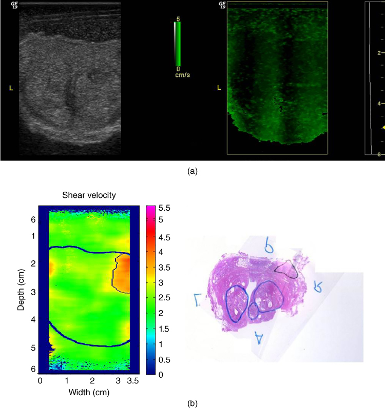
Figure 15.5 Crawling waves in the prostate. (a), left: B‐scan of whole excised prostate; right: crawling waves frame; (b), right: pathology with labels: upper triangle = cancer and lower ovals = benign prostatic hyperplasis (BPH); left: quantitative estimates of shear velocity from crawling waves analysis, indicating the hard region as a upper right area (corresponding to the region with cancer). Estimates from an average of three frequencies are shown. All images are co‐registered..
Source: Anastasio and La Riviere [4], Figure 12.8, p. 190; reproduced with permission from Taylor and Francis Group
Other applications of crawling waves include quantification of the elastic properties of muscle [42, 43], thyroid [44], and fatty livers [45–48].
15.6 Conclusion
There are a number of key advantages to “sonoelastography” imaging and crawling waves imaging. First, in sinusoidal steady‐state shear wave excitation, the amplitude contrast effect (of stiff lesions) can be seen with any Doppler imaging platform; it is not necessary to have any synchronization system or specialized platform [49]. Second, by proper choice of shear wave frequency, entire organs can be covered with shear waves, providing large ROIs for analysis [3]. This fact has been used to great advantage in MRE, as well. Finally, the crawling waves approach provides data that can be analyzed with a number of simple local estimators, while producing comparable resolution and accuracy to the very best shear wave tracking approaches using radiation force excitations [50]. In addition, the crawling waves patterns can be produced simply by external transducers [18, 28] or by an alternating pair of radiation force beams, one on the right and on the left of the ROI [51, 52]. Thus these techniques are widely applicable and efficacious for studies of tissue elastography in the breast, liver, thyroid, muscle, and other soft tissues.
Acknowledgments
This work was supported by the Hajim School of Engineering and Applied Sciences at the University of Rochester, and by National Institutes of Health grants R01 AG016317 and R01 AG029804.
References
- 1 Lerner, R.M. and Parker, K.J. (1987). Sonoelasticity images derived from ultrasound signals in mechanically vibrated targets. In Seventh European Communities Workshop (ed. J. Tjissen). Nijmegen, The Netherlands.
- 2 Lerner, R.M., Parker, K.J., Holen, J., et al. (1988). Sonoelasticity: medical elasticity images derived from ultrasound signals in mechanically vibrated targets. Acoust. Imag. 16: 317–327.
- 3 Parker, K. J. and Lerner, R.M. (1992). Sonoelasticity of organs: shear waves ring a bell. J. Ultrasound Med. 11: 387–392.
- 4 Anastasio, M.A. and La Riviere, P. (2013). Emerging Imaging Technologies in Medicine. Boca Raton: CRC Press.
- 5 Lerner, R.M., Huang, S.R., and Parker, K.J. (1990). “Sonoelasticity” images derived from ultrasound signals in mechanically vibrated tissues. Ultrasound Med. Biol. 16: 231–239.
- 6 Parker, K.J., Huang, S.R., Lerner, R.M., et al. (1993). Elastic and ultrasonic properties of the prostate. In: Proceeding of the 1993 Ultrasonics Symposium, 1032: 1035–1038.
- 7 Parker, K.J., Huang, S.R., Musulin, R.A., and Lerner, R.M. (1990). Tissue response to mechanical vibrations for “sonoelasticity imaging”. Ultrasound Med. Biol. 16: 241–246.
- 8 Taylor, L.S., Porter, B.C., Rubens, D.J., and Parker, K.J. (2000). Three‐dimensional sonoelastography: principles and practices. Phys. Med. Biol. 45: 1477–1494.
- 9 Gao, L., Parker, K.J., Alam, S.K., and Lernel, R.M. (1995). Sonoelasticity imaging: theory and experimental verification. J. Acoust. Soc. Am. 97: 3875–3886.
- 10 Parker, K.J., Fu, D., Graceswki, S.M., et al. (1998). Vibration sonoelastography and the detectability of lesions. Ultrasound Med. Biol. 24: 1437–1447.
- 11 Huang, S.R., Lerner, R.M., and Parker, K.J. (1990). On estimating the amplitude of harmonic vibration from the doppler spectrum of reflected signals. J. Acoust. Soc. Am. 88: 2702–2712.
- 12 Huang, S.R., Lerner, R.M., and Parker, K.J. (1992). Time domain Doppler estimators of the amplitude of vibrating targets. J. Acoust. Soc. Am. 91: 965–974.
- 13 Parker, K.J., Taylor, L.S., Gracewski, S., and Rubens, D.J. (2005). A unified view of imaging the elastic properties of tissue. J. Acoust. Soc. Am. 117: 2705–2712.
- 14 Yamakoshi, Y., Sato, J., and Sato, T. (1990). Ultrasonic imaging of internal vibration of soft tissue under forced vibration. IEEE Trans. Ultrason., Ferroelect., Freq. Control 37: 45–53.
- 15 Levinson, S.F., Shinagawa, M., and Sato, T. (1995). Sonoelastic determination of human skeletal‐muscle elasticity. J. Biomech. 28: 1145–1154.
- 16 Wu, Z., Taylor, L.S., Rubens, D.J., and Parker, K.J. (2004). Sonoelastographic imaging of interference patterns for estimation of the shear velocity of homogeneous biomaterials. Phys. Med. Biol. 49: 911–922.
- 17 Wu, Z. (2005). Shear wave interferometry and holography, an application of sonoelastography. In: Electrical & Computer Engineering, 104. University of Rochester, Rochester, NY.
- 18 Wu, Z., Hoyt, K., Rubens, D.J., and Parker, K.J. (2006). Sonoelastographic imaging of interference patterns for estimation of shear velocity distribution in biomaterials. J. Acoust. Soc. Am. 120: 535–545.
- 19 Wu, Z., Taylor, L.S., Rubens, D.J., and Parker, K.J. (2002). Shear wave focusing for three‐dimensional sonoelastography. J. Acoust. Soc. Am. 111: 439–446.
- 20 Zhang, M., Castaneda, B., Wu, Z., et al. (2007). Congruence of imaging estimators and mechanical measurements of viscoelastic properties of soft tissues. Ultrasound Med. Biol. 33: 1617–1631.
- 21 Hoyt, K., Castaneda, B., and Parker, K.J. (2007). Feasibility of two‐dimensional quantitative sonoelastographic imaging. In: Proceedings of the 2007 Ultrasonics Symposium, 2032–2035.
- 22 Hoyt, K., Castaneda, B., and Parker, K.J. (2008). Two‐dimensional sonoelastographic shear velocity imaging. Ultrasound Med. Biol. 34: 276–288.
- 23 Hoyt, K., Parker, K.J., and Rubens, D.J. (2007). Real‐time shear velocity imaging using sonoelastographic techniques. Ultrasound Med. Biol. 33: 1086–1097.
- 24 McLaughlin, J., Renzi, D., Parker, K., and Wu, Z. (2007). Shear wave speed recovery using moving interference patterns obtained in sonoelastography experiments. J. Acoust. Soc. Am. 121: 2438–2446.
- 25 An, L., Rubens, D.J., and Strang, J. (2010). Evaluation of crawling wave estimator bias on elastic contrast quantification. In: American Institute of Ultrasound in Medicine Annual Convention, S1–14. San Diego, CA.
- 26 Cho, Y.T., Hah, Z., and An, L. (2010). Theoretical investigation of strategies for generating crawling waves using focused beams. In: American Institue for Ultrasound in Medicine Annual Convention, S1–14. San Diego, CA.
- 27 Hah, Z., Hazard, C., Cho, Y.T., et al. (2010). Crawling waves from radiation force excitation. Ultrason. Imaging 32: 177–189.
- 28 Partin, A., Hah, Z., Barry, C.T., et al. (2014). Elasticity estimates from images of crawling waves generated by miniature surface sources. Ultrasound Med. Biol. 40: 685–694.
- 29 Alam, S.K., Richards, D.W., and Parker, K.J. (1994). Detection of intraocular pressure change in the eye using sonoelastic Doppler ultrasound. Ultrasound Med. Biol. 20: 751–758.
- 30 Rubens, D.J., Hadley, M.A., Alam, S. K., et al. (1995). Sonoelasticity imaging of prostate cancer: in vitro results. Radiology 195: 379–383.
- 31 Castaneda, B., Hoyt, K., Zhang, M., et al. (2007). P1C‐9 Prostate cancer detection based on three dimensional sonoelastography. In: Proceedings of the 2007 Ultrasonics Symposium, 1353–1356.
- 32 Taylor, L.S., Gaborski, T.R., Strang, J.G., et al. (2002). Detection and three‐dimensional visualization of lesion models using sonoelastography. In: SPIE Medical Imaging 2002: Ultrasonic Imaging and Signal Processing (ed. M. F. Insana and W. F. Walker), 421–429.
- 33 Taylor, L.S., Rubens, D.J., Porter, B.C. et al. (2005). Prostate cancer: three‐dimensional sonoelastography for in vitro detection. Radiology 237: 981–985.
- 34 Zhang, M., Nigwekar, P., Castaneda, B., et al. (2008). Quantitative characterization of viscoelastic properties of human prostate correlated with histology. Ultrasound Med. Biol. 34: 1033–1042.
- 35 Castaneda, B., Tamez‐Pena, J.G., and Zhang, M., (2008). Measurement of thermally‐ablated lesions in sonoelastographic images using level set methods. In Proc SPIE 2008 (ed. S. A. McAleavey and J. D'hooge), 692018‐692011‐692018‐692018.
- 36 Castaneda, B., Zhang, M., Hoyt, K., et al. (2007). P1C‐4 real‐time semi‐automatic segmentation of hepatic radiofrequency ablated lesions in an in vivo porcine model using sonoelastography. In: Proceedings of the 2007 Ultrasonics Symposium, 1341–1344.
- 37 Taylor, L.S. and Zhang, M. (2002). In‐vitro imaging of thermal lesions using three‐dimensional vibration sonoelatography. In: Second International Symposium on Therapeutic Ultrasound, 176–184.
- 38 Zhang, M., Castaneda, B., Christensen, J., et al. (2008). Real‐time sonoelastography of hepatic thermal lesions in a swine model. Med. Phys. 35: 4132–4141.
- 39 Castaneda, B., An, L., Wu, S., et al. (2009). Prostate cancer detection using crawling wave sonoelastography (ed. S. A. McAleavey and J. D'Hooge), 726513‐726511‐726513‐726510. SPIE, Lake Buena Vista, FL, USA.
- 40 Hoyt, K., Castaneda, B., Zhang, M., et al. (2008). Tissue elasticity properties as biomarkers for prostate cancer. Cancer Biomark. 4: 213–225.
- 41 Hoyt, K., Parker, K.J., and Rubens, D.J. (2006). Sonoelastographic shear velocity imaging: experiments on tissue phantom and prostate. In: Proceedings of the 2006 Ultrasonics Symposium, 1686–1689.
- 42 Hoyt, K., Kneezel, T., Castaneda, B., and Parker, K.J. (2008). Quantitative sonoelastography for the in vivo assessment of skeletal muscle viscoelasticity. Phys. Med. Biol. 53: 4063–4080.
- 43 Hoyt, K., Castaneda, B., and Parker, K.J. (2007). Muscle tissue characterization using quantitative sonoelastography: preliminary results. In: Proceedings of the 2007 Ultrasonics Symposium, 365–368.
- 44 Walsh, J., An, L., Mills, B., et al. (2012). Quantitative crawling wave sonoelastography of benign and malignant thyroid nodules. Otolaryngol. Head Neck Surg. 147: 233–238.
- 45 Barry, C.T., Hah, Z., Partin, A., et al. (2014). Mouse liver dispersion for the diagnosis of early‐stage fatty liver disease: a 70‐sample study. Ultrasound Med. Biol. 40: 704–713.
- 46 Barry, C.T., Hazard, C., Hah, Z., et al. (2015). Shear wave dispersion in lean versus steatotic rat livers. J. Ultrasound Med. 34: 1123–1129.
- 47 Barry, C.T., Mills, B., Hah, Z., et al. (2012). Shear wave dispersion measures liver steatosis. Ultrasound Med. Biol. 38: 175–182.
- 48 Parker, K.J., Partin, A., and Rubens, D.J. (2015). What do we know about shear wave dispersion in normal and steatotic livers? Ultrasound Med. Biol. 41: 1481–1487.
- 49 Torres, G., Chau, G.R., Parker, K.J., et al. (2016). Temporal artifact minimization in sonoelastography through optimal selection of imaging parameters, J. Acoust. Soc. Am. 140: 714–717.
- 50 Ormachea, J., Lavarello, R.J., McAleavey, S.A., et al. (2016). Shear wave speed measurements using crawling wave sonoelastography and single tracking location shear wave elasticity imaging for tissue characterization. IEEE Trans. Ultrason., Ferroelect., Freq. Control. 63: 1351–1360.
- 51 Hah, Z., Hazard, C., Mills, B., et al. (2012). Integration of crawling waves in an ultrasound imaging system. part 2: signal processing and applications. Ultrasound Med. Biol. 38: 312–323.
- 52 Hazard, C., Hah, Z., Rubens, D., and Parker, K. (2012). Integration of crawling waves in an ultrasound imaging system. part 1: system and design considerations. Ultrasound Med. Biol. 38: 296–311.