27
Application of Guided Waves for Quantifying Elasticity and Viscoelasticity of Boundary Sensitive Organs
Sara Aristizabal1, Matthew Urban2, Luiz Vasconcelos3, Benjamin Wood3, Miguel Bernal4, Javier Brum5 and Ivan Nenadic3
1 Well Living Lab, Rochester, MN, USA
2 Department of Radiology, Mayo Clinic, Rochester, MN, USA
3 Department of Physiology and Biomedical Engineering, Mayo Clinic, Rochester, MN, USA
4 Universidad Pontificia Bolivariana, Medellín, Colombia
5 Laboratorio deAcustica Ultrasonora, Instituto de Fisica, Facultad de Ciencias, Universidad de la Republica, Montevideo, Uruguay
27.1 Introduction
The field of shear wave elastography has offered numerous techniques to quantify the viscoelastic properties of various biological tissues such as kidneys, myocardium, breast, liver, prostate, and others [1–3]. The majority of these methods assume the presence of a “pure” shear wave and relate the observed shear wave velocity (c) to the shear modulus of elasticity (μ) via μ = c 2 ρ, where ρ is tissue density (around 1000 kg/m3). The pure shear wave assumption is appropriate for tissues such as the liver, kidneys, and breast tissue (often referred to as bulky organs) when the shear waves propagate in the middle of the organ and do not reflect from the organ boundaries. In bulky organs, the focused radiation force excites shear waves and compressional waves that attenuate before they reach the edges of the medium, and therefore do not form an interference pattern. In organs such as the arteries, myocardial free wall, bladder, cornea, and tendons, this assumption is not appropriate [4] because the compressional and shear waves create an interference pattern resulting in types of shear waves that are traditionally modeled as Lamb and Rayleigh waves [5–7]. These organs are referred to as boundary sensitive media and the application of shear wave elastography methods in these organs requires additional theoretical consideration. The theoretical basis of guided waves in boundary sensitive media has been described in greater detail in Chapter of this textbook (Transverse Wave Propagation in Bounded Media). Here, we briefly revisit the theory and summarize experimental results of in vivo application of guided waves in the viscoelastic assessment of the myocardium, large arteries, bladder, cornea, and tendons.
27.2 Myocardium
The general theory of wave propagation in boundary sensitive media has been laid out in Chapter of this textbook (Transverse Wave Propagation in Bounded Media). Here, we briefly summarize the basic concepts and build on the previously presented work. Most techniques mentioned in this chapter rely on the anti‐symmetric Lamb wave theory [8, 9].
Kanai [10] originally presented an anti‐symmetric Lamb wave model used to represent the motion of the septal myocardium due to aortic‐valve closure. The myocardium was modeled as a homogenous viscoelastic plate composed of a Voigt material so that the shear modulus ![]() , where
, where ![]() and
and ![]() are the shear elasticity and viscosity, respectively. Additionally, this plate is considered to be surrounded by fluid on both edges. Assuming that the bulk modulus is much larger than the shear modulus, the anti‐symmetric Lamb wave model requires the following equation to hold
are the shear elasticity and viscosity, respectively. Additionally, this plate is considered to be surrounded by fluid on both edges. Assuming that the bulk modulus is much larger than the shear modulus, the anti‐symmetric Lamb wave model requires the following equation to hold
where ![]() is the Lamb wave number,
is the Lamb wave number, ![]() is the angular frequency,
is the angular frequency, ![]() is the frequency‐dependent Lamb wave velocity,
is the frequency‐dependent Lamb wave velocity, ![]() ,
, ![]() is the shear wave number,
is the shear wave number, ![]() is the density of the sample, and h is the half‐thickness of the sample. In order to obtain the elasticity and viscosity coefficients
is the density of the sample, and h is the half‐thickness of the sample. In order to obtain the elasticity and viscosity coefficients ![]() and
and ![]() Eq. is fitted to the Lamb wave dispersion curves (velocity versus frequency).
Eq. is fitted to the Lamb wave dispersion curves (velocity versus frequency).
The myocardium is a soft tissue subject to the propagation of guided waves along its length. The thickness of the heart wall with respect to the shear wavelength can affect the velocity of propagation of shear waves, giving rise to guided waves which depend on both the geometry and the properties of the tissue. Alterations in the normal structure of the myocardium can change the tissue properties and function, hence the importance of developing a method that can assess the mechanical properties of the myocardial tissue noninvasively.
The left ventricular (LV) free myocardium is 10–20 mm thick and it can be considered in the same order of the magnitude of the focal length of the acoustic radiation force for many applications. The myocardium is characterized by being surrounded by blood and pericardial fluid on either side of it and can therefore be modelled as a solid plate submerged in fluid. Kanai [10] used a high sensitivity ultrasound method to detect shear wave propagation in the myocardial septum due to closure of the aortic valve. The motion of the septum was modeled by an antisymmetric plane Lamb wave in an infinite isotropic plate with incompressible fluid on both sides. This method was used to measure shear wave dispersion in the frequency range 10–90 Hz and fit the Lamb wave model to estimate elasticity and viscosity. Nenadic et al. proposed a similar method to measure the dispersion of anti‐symmetric Lamb waves in the myocardium, called the Lamb wave dispersion ultrasound vibrometry method (LDUV) [8]. LDUV measures the velocity dispersion as a function of frequency of anti‐symmetric Lamb waves in the tissue of interest. The principle of LDUV is shown in Figure 27.1.
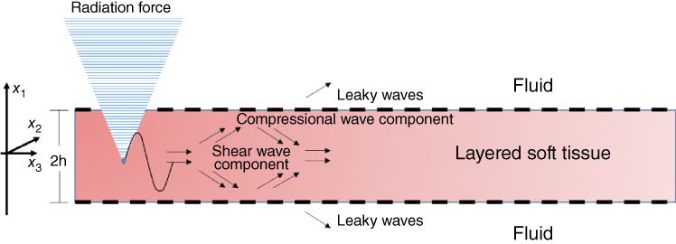
Figure 27.1 Acoustic radiation force is applied to a plate surround by fluid to make both shear and compressional waves which give rise to the Lamb waves. The same transducer used to generate the acoustic radiation force can then be switched to pulse‐echo mode for motion detection or another transducer can be used. The pulse‐echo interrogation is used to measure the resulting wave motion.
A cross‐spectral analysis or other type of analysis can be performed to calculate the motion as a function of time and the velocity is measured by calculating the phase shift over the distance of wave propagation [11, 12]. An antisymmetric Lamb wave model is then fitted to velocity dispersion data to estimate the elasticity and viscosity. An example in a rubber plate phantom is shown in Figure 27.2.
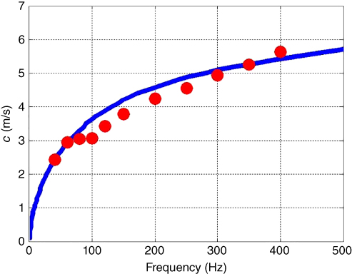
Figure 27.2 Lamb wave dispersion in a urethane rubber plate: experimentally obtained shear wave dispersion curves are shown as circles. Lamb wave model (solid line) was fitted to the data to obtain the values of elasticity and viscosity μ 1 = 45.1 kPa and μ 2 = 6.5 Pa·s. © Institute of Physics and Engineering in Medicine. Source: reproduced by permission of IOP Publishing, all rights reserved [8].
The LDUV method was used in ex vivo myocardial samples and the ranges of the viscoelastic parameters were μ 1 = 15–18 kPa and μ 2 = 5–7 Pa·s [8]. Nenadic et al. performed in vivo experiments of Lamb wave propagation in pig hearts using a transthoracic approach [13]. For these studies, the wave excitation was triggered by electrocardiographic (ECG) R‐wave and the data was acquired during an entire heart cycle. The elasticity and viscosity of the myocardium were estimated by fitting Eq. to the dispersion curves throughout the heart cycle. In these transthoracic measurements, the average group velocity, elasticity, and viscosity showed a similar pattern of increase in systole and decrease in diastole, consistent with the ECG signal, as shown in Figures. 27.3c, 27.3d, and 27.3e respectively.
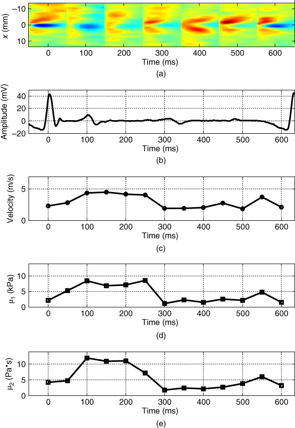
Figure 27.3 R‐wave ECG‐gated transthoracic measurements of Lamb wave group velocity, elasticity, and viscosity in a beating porcine left ventricular free wall averaged over 5–10 acquisitions. Average group velocity (c), elasticity (d), and viscosity (e) show a similar pattern of increase in systole and decrease in diastole, consistent with the ECG signal. Source: © Institute of Physics and Engineering in Medicine, reproduced by permission of IOP Publishing, all rights reserved [32].
Group velocity changed from around 1.5 m/s in diastole to around 5 m/s in systole (Figure 27.3c). Leftward and rightward propagating waves follow the same general pattern and are fairly similar. The values of elasticity (μ 1) increased from ∼ 2 to 8 kPa, while the values of viscosity (μ 2) increased from ∼2 to 12 Pa·s from diastole to systole.
Urban et al. used the LDUV method with mechanical excitation in eight pigs in an open‐chest preparation [14]. Using a mechanical actuator, harmonic waves were generated to propagate in the myocardial wall and the velocities of wave propagation were measured in the range of 50–400 Hz over several cardiac cycles. The results of this study demonstrated that the dispersive phase velocity of the waves is consistent with an antisymmetric Lamb wave model. Additional work was done with the same method on pigs with myocardial infarction with reperfusion which demonstrated that the viscosity increased after reperfusion in diastole and systole and the shear elasticity increased in diastole after reperfusion [15]. Additionally, the LDUV method allows for the estimation of elasticity and viscosity of the myocardial wall throughout the course of the cardiac cycle.
Similar open‐chest studies have been performed by Couade et al. for the in vivo assessment of myocardial mechanical properties during the cardiac cycle. [16]. To estimate the shear modulus, ![]() , of the myocardium, the speed of propagation of the shear wave,
, of the myocardium, the speed of propagation of the shear wave, ![]() is measured and the following relationship is used to estimate
is measured and the following relationship is used to estimate ![]()

where ![]() is the density of the myocardium, which is assumed to be equal to that of water (1000 kg/m3). Couade et al. assumed that the shear waves induced using the SSI method have millimetric wavelengths and propagate only over a few millimeters, hence they are not subject to the condition of guided wave propagation since the propagation distance is not comparable to the thickness of the myocardial wall. Nevertheless, they are subjected to myocardial anisotropy.
is the density of the myocardium, which is assumed to be equal to that of water (1000 kg/m3). Couade et al. assumed that the shear waves induced using the SSI method have millimetric wavelengths and propagate only over a few millimeters, hence they are not subject to the condition of guided wave propagation since the propagation distance is not comparable to the thickness of the myocardial wall. Nevertheless, they are subjected to myocardial anisotropy.
To explore this phenomenon experiments were conducted on ten sheep. Shear waves were generated and measured at an ultrafast frame rate during an entire cardiac cycle using the supersonic shear imaging method whose principles have been described in Chapter . The measurement of elasticity was performed in a 2 cm wide region and the myocardium was imaged over its whole thickness. The speed of propagation of the shear wave was then calculated from backscattered ultrasonic echoes obtained at an ultrafast frame rate (up to 12 000 frames per second).
Figure 27.4 shows 15 wave acquisitions of 4 ms each where it is possible to appreciate the change of shear wave speed several times during the cardiac cycle. Additionally, the variation of the shear modulus of the myocardium as a function of time is shown in Figure 27.5, where it is possible to appreciate the temporal variation of ![]() for acquisitions within the same region.
for acquisitions within the same region.

Figure 27.4 (a) ECG trace registered to the acquisition (including R‐wave, T‐wave, and then P‐wave). (b) 2D spatiotemporal representation of the total particular velocity due to heart motion and shear wave induced 15 times by radiation force every 45 ms. (c) Particular velocity due to shear wave only: the heart motion is rejected by removing at each location the time average over the 4 ms length of the acquisition. (d) Time axis representing the global acquisition sequence: each blue rectangle is 4 ms wide and represents the combination of a pushing beam and an ultrafast sequence (as shown in Figure 27.2). Because the ultrafast imaging is used only every 45 ms for only 4 ms, the motion is not estimated continuously [16].

Figure 27.5 Time variation of shear modulus: four consecutive acquisitions were performed by removing/replacing the probe on the left ventricle in long axis view (mean SD). Based on coregistered ECG signal (not represented here), the time axis has been shifted for each acquisition in order to put the R‐wave peak at t = 0 [16].
27.3 Arteries
Estimating the mechanical properties of arteries has become a central role in the cardiovascular field as it has been shown to be a predictor of heart‐related diseases such as type II diabetes, hypertension, and end‐stage renal disease [17–19]. The viscoelastic properties of arteries have been widely studied over the last two decades but more recently arterial stiffness has become the subject of serious investigations to assess the progression of conditions that affect the arterial tree [20, 21]. In this chapter, we introduce the work performed by Bernal et al. and Couade et al., who have investigated the material properties of arteries using acoustic radiation force and shear wave imaging [9, 22].
Bernal et al. studied arterial elasticity by identifying the modes of wave propagation in tubes made out of urethane rubber and excised pig carotid arteries using the two‐dimensional (2D) fast Fourier transform (2D FFT) [22]. From the magnitude distribution of the k‐space of the propagating wave, the global peak is found by identifying the maximum magnitude for each temporal frequency and then determining the wavenumber, k s, associated with it. Using the values of frequency, f, and wavenumber, k s, we can calculate the dispersion curves using c = λf, where c is the velocity of the guided wave and λ is the wavelength 1/k s. The dispersion curves are then derived by finding the phase velocity for the maximum magnitude of the 2D Fourier transform at each individual frequency after filtering the interference of the arterial pulse wave from the cardiac cycle by removing the time‐averaged particle velocity of each line. The dispersion curves are then used to estimate the shear modulus of the arterial wall using a leaky zero‐order antisymmetric (A 0) Lamb wave model of propagation described elsewhere in this textbook (Chapter , Transverse Wave Propagation in Bounded Media). Urethane tubes and excised arteries were mounted in a metallic frame and embedded in tissue‐mimicking gelatin. Arteries and tubes were pressurized over a range of 10–100 mmHg. Mechanical waves were generated and measured using a focused ultrasound and measured with a pulse‐echo transducer, respectively.
To generate mechanical waves, Bernal et al. used acoustic radiation force, consisting of five tone bursts lasting 200 µs each, transmitted using a confocal transducer with center frequency of 3 MHz. Vibration of the arterial wall was measured using pulse‐echo at 21 points along the length of the artery/phantom. A cross‐spectral method was used to estimate the phase shifts between pulse‐echo measurements [11]. The dispersion curves were obtained from the k‐space representation using the 2D FFT method. The shear modulus of elasticity, ![]() , of the excised arteries and urethane tubes were estimated by fitting the first antisymmetric Lamb wave mode, A
0 in Eq. , to the dispersion curves as shown in Figure 27.6. The lower order of longitudinal guided wave propagation in tubes can be approximated by the antisymmetric Lamb wave mode in plates.
, of the excised arteries and urethane tubes were estimated by fitting the first antisymmetric Lamb wave mode, A
0 in Eq. , to the dispersion curves as shown in Figure 27.6. The lower order of longitudinal guided wave propagation in tubes can be approximated by the antisymmetric Lamb wave mode in plates.

Figure 27.6 Experimental dispersion curves and fitting of a Lamb wave model. Panel A shows the dispersion curve for the urethane tube at 50 mmHg. The black circles represent the highest energy mode while the light circles represent the peaks in the wave number direction. The dark and the light lines represent the antisymmetric (A) and symmetric (S) modes for the Lamb wave model. Similarly, panel B shows the dispersion curves and Lamb wave fitting for the artery at 50 mmHg. The legend from panel A also applies to panel B [22].
Couade et al. proposed an ultrasound method based on supersonic shear imaging (SSI) [23] to assess the arterial wall stiffness. This technique generates a broadband guided shear wave (100–1500 Hz) in the arterial wall and tracks the wave propagation using ultrafast imaging. The studied was performed using a Aixplorer (SSI) scanner programmed to perform conventional B‐mode imaging, acoustic radiation force for the generation of shear waves, and ultrafast imaging to image the propagation of shear waves at a frame rate higher than 2000 images per second.
To image the shear wave propagation in the arterial walls, the setup similar to that shown in Figure 27.1 is used, where the acoustic radiation force push and pulse‐echo detection are performed with the same transducer. The transducer is aligned with the artery during the entire process. The generated push beam is transmitted at three specific locations in depth, spaced 1 mm apart. The average focal depth is set in the center of the arterial wall. This is done to compensate for any movement due to the cardiac cycle. Each push beam has duration of 100 µs, inducing a mean wall displacement of 10 µm along the plane of the probe. After the transmission of the shear wave was complete, the probe is switched to the ultrafast mode in order to scan and acquire data of the shear wave propagation. Beamforming is performed to create the 2D images of the entire motion of the shear wave propagation using the ultrasonic backscattered echoes (RF data). The wave's axial velocity is estimated via an in‐phase/quadrature (IQ) auto‐correlation of frame‐by‐frame motion detection [12]. Images are then stitched to create a “movie” of the axial velocity at a frame rate of 8000 images/second similar in appearance to Figures 27.7 and 27.8. The velocity of the shear wave in the arterial wall could then be extracted using Eq. , where x is the line number, t is the frame number, and r wall(x, t) is the detected position of the arterial wall at a specific line and frame number. Data from an experiment in a phantom is shown in Figure 27.7. In vivo measurements in the carotid artery are shown in Figure 27.8.
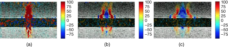
Figure 27.7 Shear wave propagation along the superior wall of an arterial phantom (agar gel) embedded into softer gelatin gel. The axial velocity field (tissue Doppler imaging) is superimposed to the anatomic grayscale image in color (mm/s) at different time steps: (a) t = 0.5 ms, (b) t = 2 ms, and (c) t = 4 ms. The ultrasonic probe is located on the top of the images. The elastic wave propagating along the wall is faster than in the surrounding softer gel [9].

Figure 27.8 In vivo experiment in the carotid artery: propagation of a shear wave generated by acoustic remote palpation and acquired by ultrafast imaging: Color‐coded axial displacements are superimposed to grayscale anatomic B‐mode and represented at (a) t = 0.5 ms, (b) t = 2 ms, and (c) t = 4 ms after the generation of the acoustic radiation force [9].
As the mechanical properties of the arterial wall can vary across the cardiac cycle, Couade et al. also showed the feasibility of generating and measuring shear waves several times per second during the cardiac cycle in order to track these changes, as shown in Figure 27.9 [9].
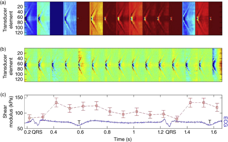
Figure 27.9 Real‐time in vivo measurement of carotid arterial wall shear modulus variation during a single heart cycle (13 values/cycle) with time‐registered ECG. (a) 15 successive space‐time representations of tissue particle velocity in the arterial wall. One clearly notices on each successive set of data the presence of a propagating wave caused by the radiation force generation. (b) The same dataset after filtering of the homogeneous velocity offset as a result of the arterial pulse wave propagation for each ultrafast acquisition. One can clearly notice that this filtering enables discriminating both waves (arterial pulse wave and radiation force‐induced wave). (c) Shear modulus deduced from each ultrafast acquisition owing to the estimation of the wave speed of the radiation force‐induced wave [9].
Additional research has been carried out to estimate the elastic properties of the arterial wall and other thin layered organs. Nguyen et al. proposed a method called shear wave spectroscopy to estimate the viscoelastic properties of organs with thickness smaller than that of the shear wavelength [24]. These types of organs behave as soft plates and therefore the shear wave propagation in these types of tissues is guided and subjected to dispersive effects. Hence, by experimentally measuring the dispersion curves in these organs, the shear modulus can be approximated in viscoelastic plates using an analytic dispersion equation derived from the Lamb wave theory for the zero‐order antisymmetric mode A0

where ![]() is the plate thickness,
is the plate thickness, ![]() is the transverse velocity, and
is the transverse velocity, and ![]() is the angular frequency. This formula provides a reasonable approximation of the shear modulus in the frequency range from 500 to 2000 Hz.
is the angular frequency. This formula provides a reasonable approximation of the shear modulus in the frequency range from 500 to 2000 Hz.
To investigate the influence of viscosity on dispersion curves, Nguyen et al. performed shear wave spectroscopy experiments using two phantoms with viscoelastic characteristics made using 5% gelatin/agar. Xanthan gum (0.5%) was added to one of the phantoms to increase the viscosity of the sample. Nguyen et al. showed that the non‐viscous plate exhibited a dispersive effect because of the guided propagation of the shear waves and no significant differences were observed in the dispersive curves for the two phantoms, indicating that wave guides tend to affect the shear wave propagation significantly and therefore it is necessary to use shear wave spectroscopy to recover the shear modulus.
27.4 Urinary Bladder
Ultrasound bladder vibrometry (UBV) is a noninvasive technique developed by Nenadic et al. that uses Lamb waves to investigate the viscoelastic properties of the bladder wall [25]. An increase in the stiffness of bladder can be associated with pathogenic processes; hence there is a need for methods to monitor the rigidity of the bladder wall to ensure the adequate functioning of the urinary system. UBV allows monitoring the properties of the bladder wall as a function of filling volumes which is analogous to urodynamic studies. Urodynamic studies are the clinical gold standard in assessing bladder function; however, this method is invasive, costly, and can cause infection due to urinary catheterization.
UBV uses an ultrasonic array transducer to generate acoustic radiation force to excite anti‐symmetric Lamb waves in the bladder wall and tracks the motion of the wave using pulse‐echo techniques. To estimate the elastic properties of the bladder using the anti‐symmetric Lamb wave theory described earlier, the bladder is modelled as an isotropic solid plate submerged in an incompressible non‐viscous fluid. Nenadic, et al. performed experiments on formalin treated ex vivo porcine bladders to induce tissue stiffness and untreated excised porcine bladders. An example of a measurement is shown in Figure 27.10. The ex vivo experiments showed that UBV can track changes of the bladder wall's elastic properties, moreover there was a high correlation between the pressure measurements and the shear modulus estimated using UBV [25].
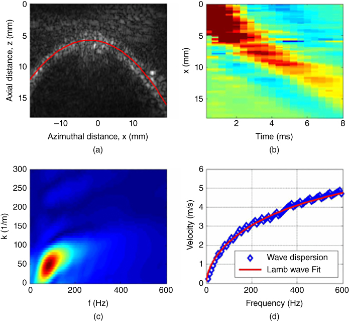
Figure 27.10 Ex vivo measurements of porcine bladder elasticity and viscosity. (a) B‐mode of bladder wall outlined in solid line. (b) Wave propagation as a function of time and distance. (c) A 2D FFT of the time and spatial signals is used to calculate the guided wave propagation dispersion. (d) The resulting phase velocity as a function of frequency is fitted with an antisymmetric wave model (Eq. ) to estimate the bladder elasticity and viscosity. Source: © Institute of Physics and Engineering in Medicine, reproduced by permission of IOP Publishing, all rights reserved [25].
Nenadic et al. also evaluated the feasibility of the UBV method for the assessment of the viscoelastic properties of the human bladder. The UBV method was performed in two patients with at least one of the following conditions: neurogenic bladder, stress incontinence, or benign prostatic hyperplasia and scheduled to undergo UDS and UBV. One of the patients was known to have a noncompliant bladder through clinical documentation while the other had a normal compliant bladder [26]. Figure 27.11 shows the mean and standard deviation of the velocity of Lamb wave propagation along the bladder wall as well as the shear modulus as a function of filling volume. The shear modulus of the noncompliant bladder was higher than that of the normal compliant bladder. The results of the clinical studies performed in in vivo bladder demonstrated that the elastic parameters estimated using UBV closely correlate with the UDS estimated data. UBV could become a potential alternative to the invasive methods for bladder compliance evaluation.
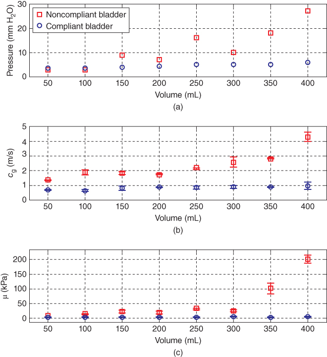
Figure 27.11 Summary of UDS and UBV comparative measurements obtained using the study design shown in Figure 27.4 in patients with a compliant (circles) and incompliant (squares) bladders. (a) UDS measurements of the detrusor pressure versus volume. (b) UBV measurements of the group velocity (c g) versus volume. (c) UBV measurements of elasticity (μ) versus volume. Source: © reproduced by permission of PLOS, all rights reserved [26].
27.5 Cornea
The assessment of the viscoelastic properties of the cornea is important for monitoring the progression of diseases such as the keratoconus, as well as a follow up strategy to evaluate the corneal biomechanical properties after patients undergo vision treatment.
Tanter et al. evaluated the feasibility of dynamic elastography to provide a map of corneal viscoelasticity using SSI. The cornea's boundary conditions can significantly affect the shear wave propagation since it can be characterized by a thin plate compared to the shear wavelength. The fact that the cornea is surrounded by a viscous fluid (aqueous humor) induces partially guided wave propagation due to reflections as the shear wave travels along the length of the cornea.
To estimate the viscoelastic properties of the corneal tissue, Tanter et al. modelled the cornea as a thin elastic plate surrounded by liquid. In this approximation, as the wave propagates along the plate it leaks energy at the wall interfaces on what is known as a “leaky” Lamb wave. Couade et al. derived an approximation for the phase velocity of this type of wave propagating in tissues (Eq. ). This approximation is then used to estimate the viscoelastic properties of the tissue from the dispersion curves, ![]() .
.
Tanter et al. evaluated fresh excised porcine eyes, placed in a positioning cap and immersed in a water bath similar to the setup in Figure 27.1 [27]. The ultrasound probe is driven by an Aixplorer system. Three pushing sequences were performed, which allowed elasticity imaging in the center and edges of the imaged area for a complete mapping of the cornea elasticity. To meet the Food and Drug Administration (FDA) requirements for ophthalmological applications, the acoustic intensity was decreased in comparison to the intensities used for organs such as the breast or muscle. Local tissue particle velocity was estimated using a 1D cross‐correlation of the successive ultrafast echographic images. The shear wave speed was subsequently estimated using a time‐of‐flight method between two points during the shear wave propagation and the shear wave group velocity was estimated over the whole shear wave bandwidth. To estimate the shear wave velocity, Tanter et al. used a shear wave spectroscopy algorithm, a Fourier transform of these signals was computed, and the ratio between wave number and frequency at each frequency peak was calculated to obtain the phase velocity. The Young's modulus is then estimated by reformulating Eq. into the form
The 2D spatial distribution of the excised corneas' relative displacements along the z‐axis as the central push is being applied is shown in Figure 27.12.
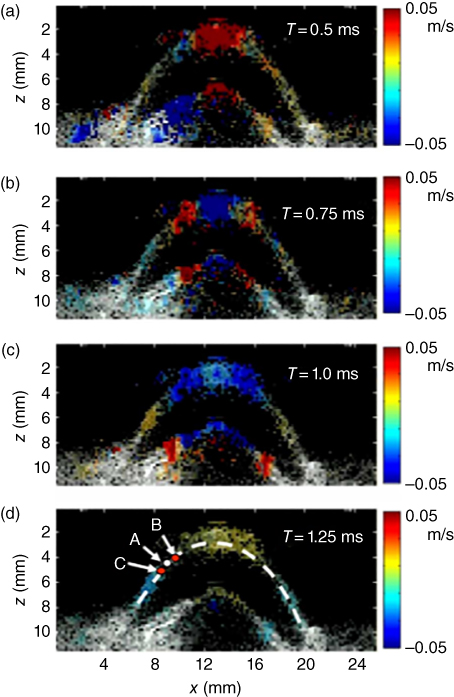
Figure 27.12 Cornea relative displacements between successive echographic images (i.e. particle velocity) at different time steps just after the ultrasonic radiation force generated at the center of the cornea. These color relative displacement images depict the shear wave propagation in the cornea and are superimposed on the echographic gray scale image. The resolution of the displacement map is 150 µm [27].
An estimate of the shear wave speed at point A outside of the pushing zone (Figure 27.13) is obtained by estimating the time delay between time profiles at points B and C surrounding point A. The choice of the distance between B and C is optimized based on the data quality (i.e. the signal‐to‐noise level of tissue displacements estimates) at A. The complete 2D mapping of the cornea using the time‐of‐flight algorithm is shown in Figure 27.13 [27].
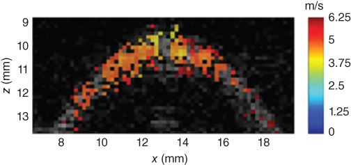
Figure 27.13 2D map of the shear wave speed superimposed on the gray scale ultrasound image of the cornea. From the knowledge of the corneal thickness (mm) and central frequency of the mechanical excitation (1500 Hz), this map can be converted into a quantitative Young's modulus map using Eq. [27].
Using the time profiles of the z‐displacement computed at each location, as shown in Figure 27.13, the Fourier transform is applied to each of them to estimate the phase of each spectral component. Finally, the dispersion curves were deduced from each pushing mode. The data was fitted to obtain the value of the Young's modulus (Figure 27.14).
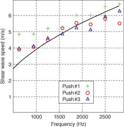
Figure 27.14 Shear wave dispersion curves estimated experimentally for the three successive mechanical waves generated by pushing modes no. 1, 2, and 3 into the porcine cornea. The solid line corresponds to Eq. [27].
This study by Tanter et al. demonstrated the ability to provide a quantitative mapping of corneal elasticity [27]. More recently, Nguyen et al. investigated the potential of corneal elasticity as a biomarker of the effectiveness of the UV‐A/riboflavin‐induced corneal collagen cross‐linking treatment (CXL) for keratoconus, a vision disorder where the round cornea undergoes a progressive thinning resulting in an irregular cone‐like shaped cornea [28]. One of the treatments available for this condition is CXL, which is a minimally invasive method to stop the progression of the keratoconus disorder and it consists of photo‐reticulating the collagen fibers of the cornea to stiffen its structure. Because there is no way to quantify the efficacy of the treatment, Nguyen et al. evaluated the biomechanical effects of CXL using corneal elasticity measured with SSI [28]. Nguyen et al. used the method previously laid out by Tanter et al. to study the biomechanical properties of ex vivo and in vivo porcine eyes using CXL experiments together with SSI. The shear wave imaging sequence consisted of four pushing beams applied along the cornea surface followed by an ultrafast imaging sequence after each push to map the entire cornea. A rubber ring was placed around the eye to enable the cornea immersion during elastography acquisition. Riboflavin 0.1% is dropped on the cornea for 20 minutes, and then the cornea was exposed to UV‐A light for 30 minutes. Anesthetized pigs were used for the in vivo studies. Elastography acquisitions were performed before and after CXL treatment with the probe placed above the cornea, as shown in Figure 27.16. The elastography measurements were triggered with the respiratory and cardiac cycle to avoid physiological displacements. The wave speed maps obtained in two corneas are shown in Figure 27.15.
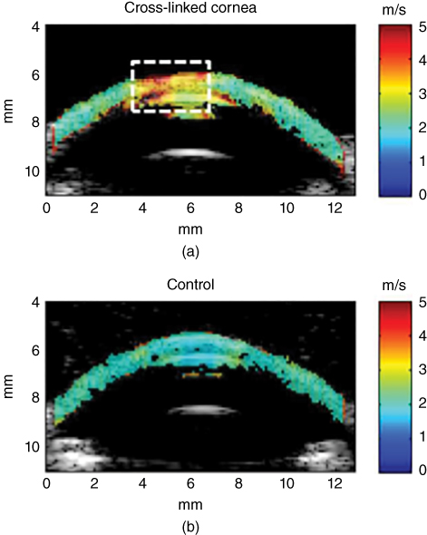
Figure 27.15 Ex vivo elastic maps acquired on porcine corneas superimposed on the echographic image. The color scale corresponds to the shear wave group velocity (m/s). A CXL was performed in vivo on the central part (delineated by the white dashed line) of the left cornea (a), while the right eye (b) of the same animal remained untreated. The color scale corresponds to the shear wave group velocity (m/s) [28].
A map of the shear wave speed of the corneal tissue obtained after the application of the CXL treatment unilaterally on the cornea can be observed in Figure 27.16. The map was obtained from the wave acquisitions in different imaging planes. The superior half of the map was stiffer than the inferior half which matches well the areas of the cornea that were treated and untreated, respectively. The work done by Nguyen et al. demonstrated the feasibility of using SSI to monitor the biomechanical changes during the CXL treatment, and it has the potential to be used immediately after CXL treatment is applied [28].
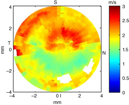
Figure 27.16 Ex vivo elastic map of the surface of the cornea after a CXL had been performed in vivo on the superior half on the cornea. The color scale corresponds to the shear group velocity (m/s). For each point, the shear wave speed has been averaged on the whole cornea thickness [28].
27.6 Tendons
Tendons are structures that attach the muscle to a bone and other structures in the human body. Tendon ruptures are associated with significant morbidity in sports and daily life and therefore it is essential to find a noninvasive technique to evaluate the elastic properties of tendons in order to predict tendon rupture and monitor the recovery.
Tendons can be described as an arrangement of collagen fibers oriented in one main direction, hence they exhibit transverse isotropic characteristics. In other words the mechanical properties of tendons are directionally dependent and the value of elasticity is different along and across the fibers. Moreover, the thickness of tendons (4 mm) is smaller than the wavelength of the shear wave, which can give rise to the propagation of guided shear waves along the tissue in the form of Lamb waves.
Brum et al. evaluated the elastic properties of tendons by studying the wave propagation along and across the fibers as a function of frequency using shear wave spectroscopy. During this study, they evaluated the right and left Achilles tendon of five healthy volunteers. Volunteers were seated with a 90° angle between the foot and the tibia and also between the tibia and the femur. The feet of the volunteers were submerged in water to facilitate the positioning of the ultrasound array. The SSI technique was applied to the tendon in the direction parallel and perpendicular to the fibers. Shear waves were generated and measured using an ultrafast ultrasound scanner. From the measured displacement shear wave, spectroscopy was applied to obtain the dispersion [29]. The results for the measurements performed along and across the fibers are shown in Figure 27.17.

Figure 27.17 Shear wave spectroscopy in the Achilles tendon for the shear wave propagation direction parallel and perpendicular to the fibers. Source: © Institute of Physics and Engineering in Medicine, reproduced by permission of IOP Publishing, all rights reserved [29].
To obtain the elastic properties of the Achilles tendon, Brum, et al. assumed the wave propagation to take place in a transverse isotropic plate surrounded by liquid (leaky Lamb wave). Moreover, Brum et al. demonstrated that guided wave propagation along the tendon fibers can be described as a superposition of anti‐symmetric and symmetric models of a transverse isotropic material. Meanwhile the propagation perpendicular to the fibers is governed by the leaky Lamb wave equation for an isotropic plate. It was found that it is essential to account for the viscosity in the direction perpendicular to the fibers, but in the parallel direction, the elasticity and viscosity are uncoupled due to strong guided wave effects. The dispersion curves obtained for two of the subjects of this study along and across the fibers are shown in Figures 27.18 and 27.19, respectively. It is possible to observe that the elastic plate behavior explains well the wave propagation along the fibers. However, this is not the case for the propagation across the fiber, where it is necessary to account for the tendons' viscosity in order to have a good estimation. Additional work on this topic has been reported by Yeh et al. and Helfenstein‐Didier et al. [30, 31].

Figure 27.18 Shear wave dispersion curves for the propagation direction parallel to the fibers. The black solid line shows the least mean square fit of the transverse isotropic plate model. Source: © Institute of Physics and Engineering in Medicine, reproduced and adapted by permission of IOP Publishing, all rights reserved [29].
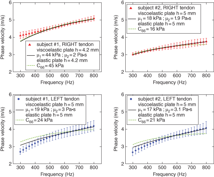
Figure 27.19 Shear wave dispersion curves for the propagation direction perpendicular to the fibers. The black solid line and the dashed line show the fit corresponding to the viscoelastic and elastic transverse isotropic plates, respectively. Source: © Institute of Physics and Engineering in Medicine, reproduced and adapted by permission of IOP Publishing, all rights reserved [29].
27.7 Conclusions
Certain organs, because of their finite thickness with respect to the shear wavelength, produce guided wave behavior. Taking into account the geometry of these organs, myocardium, arteries, bladder, cornea, and tendons, allow for quantitative estimation of the elastic and viscoelastic properties. It is important to note that the wave speed alone may not be sufficient for this full characterization, but may serve to provide some differentiation among different patients. These methods still have yet to be added to clinical machines, but the applied uses of guided waves is growing for clinical evaluation.
References
- 1 Sarvazyan, A., Hall, T.J., Urban, M.W., et al. (2011). Elasticity imaging – an emerging branch of medical imaging. An overview. Curr. Med. Imaging Rev. 7: 255–282.
- 2 Sarvazyan, A.P., Urban, M.W., and Greenleaf, J.F. (2013). Acoustic waves in medical imaging and diagnostics. Ultrasound Med. Biol. 39: 1133–1146.
- 3 Gennisson, J.L., Deffieux, T., Fink, M., and Tanter, M. (2013). Ultrasound elastography: Principles and techniques. Diagn. Interv. Imaging 94: 487–495.
- 4 Urban, M.W., Nenadic, I.Z., Chen, S., and Greenleaf, J.F. (2013). Discrepancies in reporting tissue material properties. J Ultrasound Med. 32: 886–888.
- 5 Nenadic, I.Z., Urban, M.W., Aristizabal, S., et al. (2011). On Lamb and Rayleigh wave convergence in viscoelastic tissues. Phys. Med. Biol. 56: 6723–6738.
- 6 Nenadic, I.Z., Urban, M.W., Mitchell, S.A., and Greenleaf, J.F. (2010). Inversion of Lamb waves in shearwave dispersion ultrasound vibrometry (SDUV). In: 2010 IEEE Ultrasonics Symposium, 1632–1635, San Diego, CA.
- 7 Brum, J., Gennisson, J.L., Nguyen, T.M., et al. (2012). Application of 1‐D transient elastography for the shear modulus assessment of thin‐layered soft tissue: comparison with supersonic shear imaging technique. IEEE Trans. Ultrason., Ferroelectr., Freq . Control 59: 703–714.
- 8 Nenadic, I.Z., Urban, M.W., Mitchell, S.A., and Greenleaf, J.F., (2011). Lamb wave dispersion ultrasound vibrometry (LDUV) method for quantifying mechanical properties of viscoelastic solids. Phys. Med. Biol. 56, 2245.
- 9 Couade, M., Pernot, M., Prada, C., et al. (2010). Quantitative assessment of arterial wall biomechanical properties using shear wave imaging. Ultrasound Med. Biol. 36: 1662–1676.
- 10 Kanai, H. (2005). Propagation of spontaneously actuated pulsive vibration in human heart wall and in vivo viscoelasticity estimation. IEEE Trans. Ultrason., Ferroelectr., Freq . Control 52: 1931–1942.
- 11 Hasegawa, H. and Kanai, H. (2006). Improving accuracy in estimation of artery‐wall displacement by referring to center frequency of RF echo. IEEE Trans. Ultrason., Ferroelectr., Freq . Control 53: 52–63.
- 12 Kasai, C., Namekawa, K., Koyano, A., and Omoto, R. (1985). Real‐time two‐dimensional blood flow imaging using an autocorrelation technique. IEEE Trans. Son. Ultrason. SU‐32: 458–464.
- 13 Nenadic, I.Z., Urban, M.W., Pislaru, C., et al. (2011). In vivo open and closed chest measurements of myocardial viscoelasticity through a heart cycle using Lamb wave dispersion ultrasound vibrometry (LDUV). In: 2011 International IEEE Ultrasonics Symposium, 17–20, Orlando, FL.
- 14 Urban, M.W., Pislaru, C., Nenadic, I.Z., et al. (2013). Measurement of viscoelastic properties of in vivo swine myocardium using Lamb wave dispersion ultrasound vibrometry (LDUV). IEEE Trans. Med. Imaging 32: 247–261.
- 15 Pislaru, C., Urban, M.W., Pislaru, S.V., et al. (2014). Viscoelastic properties of normal and infarcted myocardium measured by a multifrequency shear wave method: comparison with pressure‐segment length method. Ultrasound Med. Biol. 40: 1785–1795.
- 16 Couade, M., Pernot, M., Messas, E., et al. (2011). In vivo quantitative mapping of myocardial stiffening and transmural anisotropy during the cardiac cycle. IEEE Trans. Med. Imaging 30: 295–305.
- 17 Dolan, E., Thijs, L., Li, Y., et al. (2006). Ambulatory arterial stiffness index as a predictor of cardiovascular mortality in the Dublin outcome study. Hypertension 47: 365–370.
- 18 Laurent, S., Boutouyrie, P., Asmar, R., et al. (2001). Aortic stiffness is an independent predictor of all‐cause and cardiovascular mortality in hypertensive patients. Hypertension 37: 1236.
- 19 Kingwell, B.A. and Gatzka, C.D. (2002). Arterial stiffness and prediction of cardiovascular risk. J. Hypertension 20: 2337–2340.
- 20 Cameron, J.D., Bulpitt, C.J., Pinto, E.S., and Rajkumar, C. (2003). The aging of elastic and muscular arteries. Diabetes Care 26: 2133.
- 21 Duprez, D.A. and Cohn, J.N. (2007). Arterial stiffness as a risk factor for coronary atherosclerosis. Curr. Atherosclerosis Rep. 9: 139–144.
- 22 Bernal, M., Nenadic, I., Urban, M.W., and Greenleaf, J.F. (2011). Material property estimation for tubes and arteries using ultrasound radiation force and analysis of propagating modes. J. Acoust. Soc. Am. 129: 1344–1354.
- 23 Bercoff, J., Tanter, M., and Fink, M. (2004). Supersonic shear imaging: a new technique for soft tissue elasticity mapping. IEEE Trans. Ultrason., Ferroelectr., Freq . Control 51: 396–409.
- 24 Nguyen, T.‐M., Couade, M., Bercoff, J., and Tanter, M. (2011). Assessment of viscous and elastic properties of sub‐wavelength layered soft tissues using shear wave spectroscopy: Theoretical framework and in vitro experimental validation. IEEE Trans. Ultrason., Ferroelectr., Freq . Control 58: 2305–2315.
- 25 Nenadic, I.Z., Qiang, B., Urban, M.W., et al. (2013). Ultrasound bladder vibrometry method for measuring viscoelasticity of the bladder wall. Phys. Med. Biol. 58: 2675–2695.
- 26 Nenadic, I., Mynderse, L., Husmann, D., et al. (2016). Noninvasive evaluation of bladder wall mechanical properties as a function of filling volume: potential application in bladder compliance assessment. PLoS ONE 11, e0157818.
- 27 Tanter, M., Touboul, D., Gennisson, J.L., et al. (2009). High‐resolution quantitative imaging of cornea elasticity using supersonic shear imaging. IEEE Trans. Med. Imaging 28: 1881–1893.
- 28 Nguyen, T.‐M., Aubry, J.‐F., Touboul, D., et al. (2012). Monitoring of cornea elastic properties changes during UV‐A/Riboflavin‐induced corneal collagen cross‐linking using supersonic shear wave imaging: a pilot study. Invest. Ophthalmol. Vis. Sci. 53: 5948–5954.
- 29 Brum, J., Bernal, M., Gennisson, J.L., and Tanter, M. (2014). In vivo evaluation of the elastic anisotropy of the human Achilles tendon using shear wave dispersion analysis. Phys. Med. Biol. 59, 505.
- 30 Yeh, C.L., Kuo, P.L., Gennisson, J.L., et al. (2016). Shear wave measurements for evaluation of tendon diseases. IEEE Trans. Ultrason., Ferroelectr., Freq . Control 63: 1906–1921.
- 31 Helfenstein‐Didier, C., Andrade, R.J., Brum, J., et al. (2016). In vivo quantification of the shear modulus of the human Achilles tendon during passive loading using shear wave dispersion analysis. Phys. Med. Biol. 61: 2485–2496.
- 32 Nenadic, I.Z., Urban, M.W., Pislaru, C., Escobar, D., Vasconcelos, L., and Greenleaf, J.F. (2018). In vivo open‐ and closed‐chest measurements of left‐ventricular myocardial viscoelasticity using lamb wave dispersion ultrasound vibrometry (LDUV): a feasibility study, Biomed. Phys. & Eng. Express 4: 047001.