
10
Validation of Quantitative Linear and Nonlinear Compression Elastography
Jean Francois Dord1, Sevan Goenezen1, Assad A. Oberai1, Paul E. Barbone2, Jingfeng Jiang3, Timothy J. Hall4 and Theo Pavan5
1 Department of Mechanical Aerospace and Nuclear Engineering, Rensselaer Polytechnic Institute, Troy, NY, USA
2 Department of Mechanical Engineering, Boston University, Boston, MA, USA
3 Department of Biomedical Engineering, Michigan Technological University, Houghton, MI, USA
4 Medical Physics Department, University of Wisconsin, Madison, WI, USA
5 Departmento de Física, University of São Paulo, São Paulo, Brazil
10.1 Introduction
Over the last few decades elastography, or elasticity imaging, has emerged as a novel imaging modality that may be used to detect and diagnose malignant tumors 1, 2, 3. The premise behind this role for elastography is that disease often alters tissue microstructure, which in turns leads to altered macroscopic tissue properties. Most efforts in elastography have focused on recovering the linear properties of tissues 4, 5, 6 while ignoring their nonlinear behavior which becomes evident at large strains. Recent ex vivo data suggests that the nonlinear elastic behavior may play an important role in differentiating benign and malignant tissue, with the concensus being that malignant tissue tends to stiffen to a larger extent with increasing strain 7, 8, 9. This leads to the intriguing possibility of using the nonlinear behavior of tissue to discern whether a tumor is cancerous. Over the last two‐to‐three years several studies have demonstrated the feasibility of this idea 10, 11, 12, 13, 14.
Motivated by these applications we have developed and implemented an iterative, nonlinear algorithm to determine the nonlinear elastic properties of a tissue from the knowledge of its internal displacement field. We have tested this algorithm in two dimensions in the context of plane‐stress and plane‐strain approximations 15, 16. We have benchmarked its performance using synthetic (computer‐generated) displacement data. We have also applied it to a small set of patient data 27. In this chapter we benchmark the performance of this algorithm on experimentally acquired tissue‐phantom data. This allows us to work with a realistic set of measured displacements, in terms of the noise and bias introduced by the ultrasound equipment and displacement estimation algorithms, and at the same time provides a ground truth with which to compare our reconstructed material properties. We challenged our reconstruction techniques by performing a “blind” test, in that the reconstruction team was provided no information (shape, number, or contrast of inclusions) about the phantom while the modulus images are reconstructed. Once the reconstruction team delivers its “final” answer, it is compared to the experimental measurements. This answer is not modified in light of what is now known to be the correct answer. We also utilize this study as an opportunity to analyze the effect of various algorithmic choices made in our computational strategy. In particular, we examine the effect of assumed boundary conditions and the values of regularization parameters used in the inverse problem.
The layout of the remainder of this chapter is as follows. In Section 10.2 we briefly describe the solution of the inverse nonlinear elasticity problem, the ultrasound data acquisition, and the displacement estimation algorithm. Section 10.3 presents the reconstructions for the linear and nonlinear elastic parameters for the tissue‐phantom. The following section discusses several algorithmic choices for our reconstruction algorithms. Finally in Section 10.5 we discuss these results and end with conclusions.
10.2 Methods
10.2.1 The Inverse Algorithm
The inversion strategy uses a quasi‐Newton optimization algorithm (L‐BFGS‐B 28, 29) coupled with a nonlinear finite element code. The objective function is given by the sum of a data matching term and total variation (TV) regularization terms 11, 15:
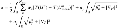
In the equation above ![]() is the
is the ![]() ‐th measured displacement field,
‐th measured displacement field, ![]() is the corresponding predicted displacement field which satisfies the equations of equilibrium for a hyperelastic material,
is the corresponding predicted displacement field which satisfies the equations of equilibrium for a hyperelastic material, ![]() is a diagonal matrix whose values are selected to emphasize the displacement components that are measured accurately, and
is a diagonal matrix whose values are selected to emphasize the displacement components that are measured accurately, and ![]() is a weight related to the amplitude of
is a weight related to the amplitude of ![]() . It is selected so that measurements made at disparate levels of strain contribute in equal measure to the data‐matching terms. The material parameters are denoted by
. It is selected so that measurements made at disparate levels of strain contribute in equal measure to the data‐matching terms. The material parameters are denoted by ![]() and
and ![]() , which denote the shear modulus at zero strain and nonlinear parameter distributions, respectively. Finally,
, which denote the shear modulus at zero strain and nonlinear parameter distributions, respectively. Finally, ![]() and
and ![]() are small constants that ensure the differentiability of the regularization terms at the origin;
are small constants that ensure the differentiability of the regularization terms at the origin; ![]() and
and ![]() are the regularization parameters associated with
are the regularization parameters associated with ![]() and
and ![]() , respectively. These parameters determine the relative importance of the data matching and the regularization terms. We note that a change in the material parameters leads to a change in the predicted displacements
, respectively. These parameters determine the relative importance of the data matching and the regularization terms. We note that a change in the material parameters leads to a change in the predicted displacements ![]() which in turn leads to a chance in the functional
which in turn leads to a chance in the functional ![]() . The goal is to find the distribution of the material parameters that minimizes
. The goal is to find the distribution of the material parameters that minimizes ![]() .
.
We model the material (gel) as an incompressible hyperelastic material. The stress‐strain behavior is thus completely determined by the strain energy density function given by

In the equation above ![]() is the shear modulus at small strains and
is the shear modulus at small strains and ![]() represents the rate of increase of stiffness with strain. In addition
represents the rate of increase of stiffness with strain. In addition ![]() and
and ![]() are the invariants of the two‐dimensional Cauchy‐Green strain tensor
are the invariants of the two‐dimensional Cauchy‐Green strain tensor ![]() . We note that the expression for the strain energy density we have used is the restriction of a simplified Veronda‐Westmann model 15, 30 to plane stress.
. We note that the expression for the strain energy density we have used is the restriction of a simplified Veronda‐Westmann model 15, 30 to plane stress.
At every iteration the quasi‐Newton algorithm requires the gradient vector which represents the change in ![]() corresponding to a change in
corresponding to a change in ![]() or
or ![]() at a spatial location. This vector is computed efficiently by utilizing the adjoint elasticity equations and a continuation strategy in material parameters 15, 16.
at a spatial location. This vector is computed efficiently by utilizing the adjoint elasticity equations and a continuation strategy in material parameters 15, 16.
10.2.2 Phantom Description and RF Data Acquisition
A phantom containing four spherical inclusions was manufactured using previously reported ultrasound phantom materials with nonlinear elastic properties 17. The methods for manufacturing phantoms with coplanar spherical inclusions were also previously reported 18, 19. Sketches of the phantom identifying the background layers and individual targets are provided in Figure 10.1. The assembled phantom is a 100 mm cube. Each spherical target is 10 mm diameter. They are separated by 30 mm (center‐to‐center) and are placed 35 mm (center to phantom edge) from the top and each lateral side of the phantom.

Figure 10.1 Three dimensional depiction of the phantom. (a) Parts that composed the phantom; (b) the phantom in its final form.
When the phantom components were manufactured, a test cylinder of the same material was also cast to provide identical material with simple geometry to independently test the stress–strain behavior of the material. Mechanical tests were performed with an EnduraTEC ELF 3200 (Bose‐EnduraTEC Systems Corporation, Minnetonka, MN, USA) using a 1 kg load cell and ![]() platens larger than the sample surface. Each test cylinder was stored in oil to prevent desiccation, and that oil was used to lubricate the platens for the mechanical testing. During the mechanical testing, the upper platen was first lowered to make contact with the test cylinder. Then, the platen was lowered further (at 0.04 mm/s) to the center of the cyclic deformation range used for material characterization and the platen remained at that deformation for 5 s. A 1 Hz oscillatory compressive load (ranging from 1% to 25% strain) was applied for 5 s before starting data acquisition to precondition the sample 20, 21. Following the preconditioning step, force and displacement data were acquired for the randomized range of displacement magnitudes for each phantom material. Thus, the stress–strain curve of each tissue‐mimicking material (2 backgrounds and 4 inclusions) was obtained and subsequently fitted to the modified Veronda‐Westmann model to estimate the small strain shear modulus
platens larger than the sample surface. Each test cylinder was stored in oil to prevent desiccation, and that oil was used to lubricate the platens for the mechanical testing. During the mechanical testing, the upper platen was first lowered to make contact with the test cylinder. Then, the platen was lowered further (at 0.04 mm/s) to the center of the cyclic deformation range used for material characterization and the platen remained at that deformation for 5 s. A 1 Hz oscillatory compressive load (ranging from 1% to 25% strain) was applied for 5 s before starting data acquisition to precondition the sample 20, 21. Following the preconditioning step, force and displacement data were acquired for the randomized range of displacement magnitudes for each phantom material. Thus, the stress–strain curve of each tissue‐mimicking material (2 backgrounds and 4 inclusions) was obtained and subsequently fitted to the modified Veronda‐Westmann model to estimate the small strain shear modulus ![]() and the nonlinear parameter
and the nonlinear parameter ![]() (see Eq. 10.2).
(see Eq. 10.2).
During phantom experiments, radiofrequency (RF) data were acquired using a Siemens SONOLINE Antares (Siemens Medical Solutions USA, Inc, Malvern, PA) clinical ultrasound system with a linear array ultrasound transducer (Siemens VFX9‐4) pulsed at 8.89 MHz. Details of the URI and bandwidth of the Siemens system are given by Brunke et al. 22. A large (approximately 15 cm by 15 cm) compression plate was attached to the ultrasound transducer to ensure nearly uniaxial deformations of the phantom. More specifically, ultrasound RF data were acquired for every 1.5% increment deformation (after the first few frames of 0.5% strain) up to approximately 20% (with respect to its height). Further details regarding this phantom are reported by Pavan et al. 23.
10.2.3 Displacement Estimation
To obtain large deformations (approximately 20%) required for nonlinear elasticity imaging, we first tracked motion sequentially through multiple frames similar to the multi‐compression technique 24. In the first step, offline motion tracking using RF echo data acquired from the nonlinear tissue‐mimicking phantom was performed between each pair of two adjacent RF echo frames [e.g. from the ![]() ‐th frame to the (
‐th frame to the (![]() )‐th frame] using a modified block‐matching algorithm 25. This modified block‐matching algorithm combines smoothness‐constrained motion tracking with predictive search 26. Specifically, this modified block‐matching algorithm first estimated reliable motion within a small neigborbood to obtain high quality displacement estimates in a sparse grid (e.g. every 5 mm). Then, these reliable high quality displacements were used as seeds to perform predictions for its immediate neighbors. During this process, a small (approximately 0.5 mm [height] by 1 mm [width]) tracking kernel was first used to obtain integer displacements. Then, sub‐sample displacement estimates (necessary for modulus inversion) were obtained with quadratic interpolations. Collectively, this algorithm significantly reduces the occurance of large motion tracking errors between two adjacent RF frames. Once all displacement fields between adjacent RF echo frames were obtained, we mapped all displacement estimates in this sequence (from the first frame to the
)‐th frame] using a modified block‐matching algorithm 25. This modified block‐matching algorithm combines smoothness‐constrained motion tracking with predictive search 26. Specifically, this modified block‐matching algorithm first estimated reliable motion within a small neigborbood to obtain high quality displacement estimates in a sparse grid (e.g. every 5 mm). Then, these reliable high quality displacements were used as seeds to perform predictions for its immediate neighbors. During this process, a small (approximately 0.5 mm [height] by 1 mm [width]) tracking kernel was first used to obtain integer displacements. Then, sub‐sample displacement estimates (necessary for modulus inversion) were obtained with quadratic interpolations. Collectively, this algorithm significantly reduces the occurance of large motion tracking errors between two adjacent RF frames. Once all displacement fields between adjacent RF echo frames were obtained, we mapped all displacement estimates in this sequence (from the first frame to the ![]() ‐th frame) to the coordinate system of the first echo frame by using B‐spline interpolations.
‐th frame) to the coordinate system of the first echo frame by using B‐spline interpolations.
10.3 Results
The displacement data was measured on a ![]() grid with a resolution of
grid with a resolution of ![]() mm. It was found that the data close to the boundaries contained more noise than inside the domain. As a result 39 lines were removed from the axial edge close to the ultrasound probe and 8 lines were removed from the opposite axial edge. In addition 9 lines were removed from each of the lateral edges. We define the axial direction to be the direction along the axis of the ultrasound transducer. The lateral direction is the direction in the imaging plane that is perpendicular to the axial direction. In order to keep the problem small the displacement field was downsampled by a factor of four in each direction. The shear modulus and nonlinear parameter images were generated on a
mm. It was found that the data close to the boundaries contained more noise than inside the domain. As a result 39 lines were removed from the axial edge close to the ultrasound probe and 8 lines were removed from the opposite axial edge. In addition 9 lines were removed from each of the lateral edges. We define the axial direction to be the direction along the axis of the ultrasound transducer. The lateral direction is the direction in the imaging plane that is perpendicular to the axial direction. In order to keep the problem small the displacement field was downsampled by a factor of four in each direction. The shear modulus and nonlinear parameter images were generated on a ![]() mesh with a resolution of
mesh with a resolution of ![]() mm. The displacement measurements were sampled on the same grid. It was recognized that the measured data in the axial direction (
mm. The displacement measurements were sampled on the same grid. It was recognized that the measured data in the axial direction (![]() ) was much more accurate than in the lateral direction (
) was much more accurate than in the lateral direction (![]() ). As a result the latter was dropped from the displacement matching term by selecting
). As a result the latter was dropped from the displacement matching term by selecting ![]() and
and ![]() . The reconstructions were performed by a team comprising of the first four authors of this chapter without any a priori knowledge of the phantom and its properties. Further, once the comparison with experimental data was made, these reconstructions were not revisited or polished.
. The reconstructions were performed by a team comprising of the first four authors of this chapter without any a priori knowledge of the phantom and its properties. Further, once the comparison with experimental data was made, these reconstructions were not revisited or polished.
10.3.1 Description of the Forward Problem
As part of our iterative strategy a forward elasticity problem is solved at every iteration of the optimization algorithm. For the boundary conditions in the forward problem, on every edge, the axial component of the displacement was set equal to the measured displacement while in the lateral direction a traction‐free state was assumed. This implied perfect slip on the axial (the top and the bottom) edges and zero normal traction on the lateral (left and right) edges. This choice was motivated by the experimental set‐up and the fact that the measured lateral displacements were too noisy to be imposed strongly. The effect of other choices for boundary conditions was also explored and is described in Section 10.4.4. The phantom was assumed to be in a state of plane stress, which is appropriate since the phantom was not confined in the elevational direction.
10.3.2 Options for the Optimization Strategy
The material parameters ![]() and
and ![]() were determined sequentially. That is, first
were determined sequentially. That is, first ![]() was reconstructed using measurements at small deformation while keeping
was reconstructed using measurements at small deformation while keeping ![]() fixed at 0.1. Thereafter
fixed at 0.1. Thereafter ![]() was reconstructed using two displacement fields at large strains while
was reconstructed using two displacement fields at large strains while ![]() was held fixed at the previously computed value.
was held fixed at the previously computed value.
Several tests (not reported here) demonstrated that the choice of the initial value for ![]() and
and ![]() did not impact the final reconstructions provided that the initial field(s) were in a reasonable range. In this chapter, the initial fields were chosen to be uniform with a value of
did not impact the final reconstructions provided that the initial field(s) were in a reasonable range. In this chapter, the initial fields were chosen to be uniform with a value of ![]() and
and ![]() . We would like to emphasize that even though the final results are not influenced by the initial field, the rate of convergence is: not surprisingly, the closer the initial choice is to the final solution, the faster the convergence.
. We would like to emphasize that even though the final results are not influenced by the initial field, the rate of convergence is: not surprisingly, the closer the initial choice is to the final solution, the faster the convergence.
The TV regularization used in Eq. (10.1) is a linear function of the magnitude of the gradient of the fields and consequently for a given contrast in material properties it will tend to reduce the mean value of the field. Additionally, the shear modulus is recovered only to a multiplicative constant as we use only displacement data in our inverse problem. Therefore it is necessary to specify a lower bound for the optimization algorithm. In this chapter, the shear modulus and nonlinear parameter are constrained as follows: ![]() and
and ![]() . Note that we ensured that the upper bound was never obtained for both
. Note that we ensured that the upper bound was never obtained for both ![]() and
and ![]() .
.
The convergence criterion plays an important role in determining the final answer. The L‐BFGS‐B algorithm implements two stopping criteria: stop when
- the relative change in the objective function value is less than a prescribed value, or
- when value of the
 ‐norm of the projected gradient is smaller than a prescribed value.
In our experience the iterations terminated due to the first criterion and we set the tolerance to be ![]() , where
, where ![]() is the machine precision. Choosing such a small value for the tolerance leads to results that are convincingly converged. A slightly higher value could have been chosen to reduce the number of iterations.
is the machine precision. Choosing such a small value for the tolerance leads to results that are convincingly converged. A slightly higher value could have been chosen to reduce the number of iterations.
10.3.3 Shear Modulus Images
The shear modulus was reconstructed using the displacement measured with an overall strain of approximately 1.5%. The results are shown in Figure 10.2 and the values of the regularization parameters appear in Table 10.1. The robustness of this strategy was verified by using one or more displacement fields with overall strain in the range of ![]() to
to ![]() in order to recover the shear modulus. It was found that this choice did not significantly change the results.
in order to recover the shear modulus. It was found that this choice did not significantly change the results.
Table 10.1 Values of the parameters for the reconstructions (Eq. 10.1).
| Parameter | set 1 | set 2 | set 3 | set 4 |
|
|
7e‐5 | 4e‐5 | 4e‐5 | 1e‐5 |
|
|
6e‐3 | 6e‐3 | 6e‐3 | 3e‐3 |
|
|
4e‐4 | 4e‐4 | 7e‐5 | 1e‐4 |
|
|
7e‐3 | 7e‐3 | 7e‐3 | 7e‐3 |

Figure 10.2
Shear modulus  reconstructions for sections 1 through 4 (left to right).
10.3.4 Nonlinear Parameter Images
The nonlinear mechanical behavior can only be observed for rather large deformations and therefore it is appropriate to use deformation states where the strain is around ![]() . Figure 10.3 shows the non linear parameter fields obtained when frames 30 (with
. Figure 10.3 shows the non linear parameter fields obtained when frames 30 (with ![]() overall strain) and 36 (with
overall strain) and 36 (with ![]() overall strain) are used. Note that, since these strains are close to each other, the weights
overall strain) are used. Note that, since these strains are close to each other, the weights ![]() in Eq. ( 10.1) are identical and equal to unity. As for the shear modulus, the values of the regularization parameters are given in Table 10.1.
in Eq. ( 10.1) are identical and equal to unity. As for the shear modulus, the values of the regularization parameters are given in Table 10.1.
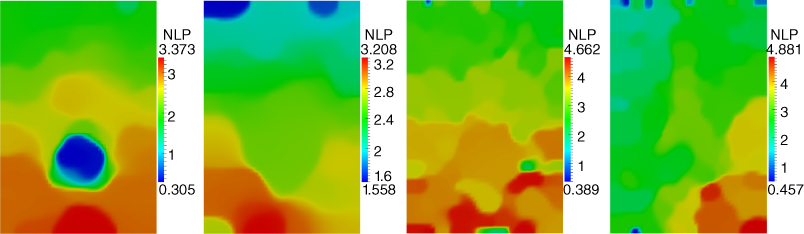
Figure 10.3
Non linear parameter  reconstructions for sections 1 through 4 (left to right).
10.3.5 Axial Strain Images
The displacement data used in generating the shear modulus and nonlinear parameter images was also used to generate axial strain images. This lead to two strain images for each section of the phantom, at approximately ![]() and
and ![]() overall strain which were evaluated using the gradient filter within Paraview 31. These images are shown in Figures 10.4 and 10.5. We observe that at small strain the strain contrast changes somewhat from one section of the phantom to another. Also, for a given section it changes rather dramatically from small to large strains.
overall strain which were evaluated using the gradient filter within Paraview 31. These images are shown in Figures 10.4 and 10.5. We observe that at small strain the strain contrast changes somewhat from one section of the phantom to another. Also, for a given section it changes rather dramatically from small to large strains.

Figure 10.4 Axial strain images at 1.5% overall strain for sections 1 through 4 (left to right).
10.4 Discussion
10.4.1 Analysis of the Shear Modulus Distributions
The shear modulus reconstructions show that every data set contains a circular inclusion in the lower part of the image. We observe that the shape and the sharp boundary of these inclusions have been recovered very accurately. The diameter of these inclusions, measured along the axial and lateral directions, is listed in Table 10.2, where we have also listed the manufactured diameter of these inclusions. We observe very good agreement too, with the maximum error of about ![]() .
.

Figure 10.5 Axial strain images at 20.5% overall strain for sections 1 through 4 (left to right).
Table 10.2 Dimensions of the inclusions after segmentation (thresholding at 30% of the maximum contrast).
| incl. 1 | incl. 2 | incl. 3 | incl. 4 | Manufactured | |
| Lateral diameter (mm) | 9.60 | 9.38 | 9.28 | 9.21 | 10.0 |
| Axial diameter (mm) | 10.87 | 10.94 | 10.74 | 10.61 | 10.0 |
| Area ( |
81.7 | 76.8 | 75.8 | 76.5 | 78.5 |
Table 10.3 Reconstructed and measured values of material properties.
| Source | incl. 1 | incl. 2 | incl. 3 | incl. 4 | backg. 1/ backg. 2 |
| Recontructed |
2.11 | 1.86 | 3.02 | 4.09 | 1 / 1.2 |
| Measured |
2.83 | 2.27 | 3.54 | 5.26 | 1 / 1.16 |
| Reconstructed |
0.35 | 2.6 | 3.8 | 2.9 | 3.4 / 2.7 |
| Measured |
2.2 | 6.5 | 4.9 | 4.5 | 4.7 / 4.3 |
With only measured displacement data, the shear modulus can be determined up to a multiplicative constant and therefore it is interesting to focus on the contrast between the inclusion and the background. The predicted and measured values are compared in Table 10.3. The measured values are obtained as described in Section 10.2.2. That is, a cylinder of each material type was compressed to obtain the uniaxial stress–strain curve, and that curve was matched to the analytical curve for the Veronda‐Westmann strain energy density function in order to determine ![]() and
and ![]() .
.
We observe that in all cases we have underestimated the contrast by about 20%. It is well known that the TV regularization results in diminishing contrast as is apparent here. Further, based on our previous experience with noisy data, a factor of 20 % appears reasonable.
We note that there is a small gradient in the shear modulus reconstruction in the axial direction. In particular the top portion of the phantom appears to be stiffer than the lower portion. We have observed the same effect in all sections and in axial strain images. This is consistent with how the phantom was manufactured in that the top portion of the background was slightly stiffer than the bottom portion (see Section 10.2.2). It is remarkable that the reconstructions are able to pick up this small effect.
10.4.2 Analysis of the Nonlinear Parameter Images
The images for the nonlinear parameter for the sections of the phantoms are shown in Figure 10.3. Here we can clearly see an inclusion only in the first section. For the other sections the inclusion is not clearly seen. This observation is consistent with the actual tissue phantom, where the background material and the inclusion material for inclusions 2, 3, and 4 was constructed to have the same nonlinear behavior. It is remarkable that our reconstructions recover this fact. Additionally, the independent mechanical measurements suggest that top background is slightly more nonlinear than bottom portion; this trend is properly captured in our reconstructions.
The measured and predicted values of the nonlinear parameter are presented in Table 10.1. We observe that, unlike with the values for the shear modulus, there is greater discrepancy between the measured and predicted values. This may be attributed to the following causes:
- In order to quantitatively recover
 and to compare the reconstructed and the measured values, as well as to compare the reconstructed values of
  across different, phantom sections, it is necessary to utilize displacement measurement at two, significantly different, levels of finite strain. In our reconstructions we have utilized displacements at
  and
and  overall strain. These may not be sufficiently different so as to measure
  quantitatively.
 - Using the formula derived in Gokhale et al. 15, see Equation (56) therein, we conclude that we require a strain of about
 in the inclusion in order to measure
  accurately. At
  overall strain we are close to, but still less than, this number. Thus the amount of total strain may not be sufficient to accurately estimate
  for the given problem.
We also note that the images for ![]() display more artifacts than the corresponding images for
display more artifacts than the corresponding images for ![]() . This may be explained by recognizing that in general the measured displacements are less sensitive to changes in
. This may be explained by recognizing that in general the measured displacements are less sensitive to changes in ![]() than in
than in ![]() 16, which makes recovering
16, which makes recovering ![]() from displacement measurements more sensitive to noise. In addition we note that
from displacement measurements more sensitive to noise. In addition we note that ![]() is recovered sequentially, that is it is based on utilizing a reconstructed (and hence noisy)
is recovered sequentially, that is it is based on utilizing a reconstructed (and hence noisy) ![]() distribution. Therefore, in addition to the noise in the measured displacements, it is also influenced by errors in the recovered
distribution. Therefore, in addition to the noise in the measured displacements, it is also influenced by errors in the recovered ![]() distribution.
distribution.
Finally, we note that strain images can be misleading when interpreting nonlinear elastic effects. A quick glance at Figures 10.4 and 10.5 might convince the reader, that relative to the background, the first two inclusions soften with strain. However, a look at the measured and reconstructed values of ![]() reveals that this not the case for the second inclusion. Only the first inclusion behaves this way, a fact that is correctly captured in the reconstruction for
reveals that this not the case for the second inclusion. Only the first inclusion behaves this way, a fact that is correctly captured in the reconstruction for ![]() .
.
10.4.3 Effect of Varying Regularization Parameters
The total variation regularization terms are the last two terms in Eq. ( 10.1). In these terms ![]() and
and ![]() are parameters that determine the importance of the regularization term relative to the data matching term while
are parameters that determine the importance of the regularization term relative to the data matching term while ![]() and
and ![]() are parameters that ensure that the integrand of the regularization terms is twice‐differentiable when
are parameters that ensure that the integrand of the regularization terms is twice‐differentiable when ![]() or
or ![]() . The idea is to select
. The idea is to select ![]() to be small enough so that they do not influence the final result, and at the same time provide the problem with enough smoothness so that quasi‐Newton methods can be used to solve it.
to be small enough so that they do not influence the final result, and at the same time provide the problem with enough smoothness so that quasi‐Newton methods can be used to solve it.
We have thoroughly investigated the effect of varying ![]() and
and ![]() on the corresponding reconstructions. In Figure 10.6 we present one such study for reconstructing the nonlinear parameter of the first specimen. We select three different values of
on the corresponding reconstructions. In Figure 10.6 we present one such study for reconstructing the nonlinear parameter of the first specimen. We select three different values of ![]() (that differ from each other by a factor of
(that differ from each other by a factor of ![]() ) while keeping all other parameters fixed. We observe that changes in the reconstructions, especially between the two images corresponding to the smaller values of
) while keeping all other parameters fixed. We observe that changes in the reconstructions, especially between the two images corresponding to the smaller values of ![]() , are minimal, indicating that we have reached an asymptotically small value for
, are minimal, indicating that we have reached an asymptotically small value for ![]() . We also observe that reducing
. We also observe that reducing ![]() adversely effects the smoothness of the problem which translates to an increase in the total number of iterations to convergence.
adversely effects the smoothness of the problem which translates to an increase in the total number of iterations to convergence.
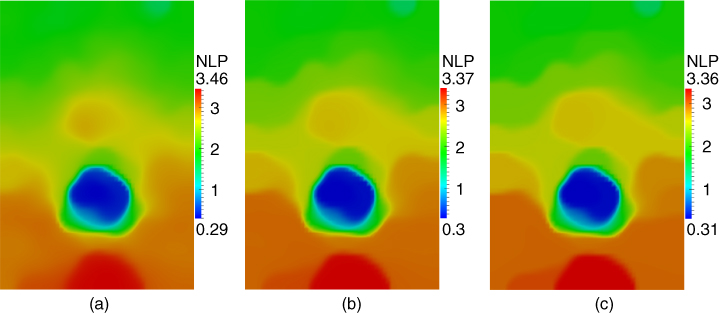
Figure 10.6
Influence of the regularization parameter  on the nonlinear parameter reconstruction for section 1. (a)
  = 4e‐2 (914 iterations to convergence); (b)
  = 7e‐3 (2214 iterations to convergence); (c)
  = 1e‐3 (5977 iterations to convergence)).
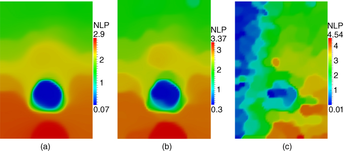
Figure 10.7
Influence of the regularization parameter  on the nonlinear parameter reconstruction for section 1. (a)
  = 1e‐3 (1852 iterations to convergence); (b)
  = 4e‐4 (2214 iterations to convergence); (c)
  = 7e‐5 (1660 iterations to convergence)).
The effect of varying the regularization parameter ![]() is shown in Figure 10.7, where we plot the reconstructed images for
is shown in Figure 10.7, where we plot the reconstructed images for ![]() for section 1 at three different values of
for section 1 at three different values of ![]() . We note that the image on the right (Figure 10.7c) is clearly under‐regularized and displays strong variations even within the homogeneous background region. The center image (Figure 10.7b) gets rid of this artifact while preserving the boundary of the inclusion. The image on the left (Figure 10.7a) has a still higher regularization parameter (around 2.5 times that for the center image). We observe that this image is similar to the center image, although the distribution for
. We note that the image on the right (Figure 10.7c) is clearly under‐regularized and displays strong variations even within the homogeneous background region. The center image (Figure 10.7b) gets rid of this artifact while preserving the boundary of the inclusion. The image on the left (Figure 10.7a) has a still higher regularization parameter (around 2.5 times that for the center image). We observe that this image is similar to the center image, although the distribution for ![]() appears to have shifted to a lower overall value. This is to be expected as this change corresponds to lowering the total variation of
appears to have shifted to a lower overall value. This is to be expected as this change corresponds to lowering the total variation of ![]() .
.
10.4.4 Effect of Boundary Conditions on Lateral Edges
While solving the forward problem we are required to specify a boundary condition in each direction on every edge. In the axial direction the measured displacements are used as boundary conditions on every edge. If we also use the measured displacement in the lateral direction as boundary data we obtain the shear modulus image for section 1 shown in Figure 10.8b. In this image we can clearly see artifacts along the edges due to the noisy lateral displacement estimates that are imposed strongly through the boundary conditions. These artifacts are somewhat mitigated by using a smoothed version of the lateral displacements, as seen in the image in Figure 10.8c. The smoothed displacement field on the boundary is obtained by linearly interpolating between 24 carefully selected points on the boundary. A point is included in this set if its lateral displacement is close to the average lateral displacement on the edge (so as to preclude outliers) and if it is sufficiently far from other points that have already been included in the selected set. Perhaps the best (in terms of a homogeneous background) reconstruction is obtained when homogeneous lateral traction is imposed (see Figure 10.8c). We note that this latter boundary condition is appropriate for our data since the phantom was not constrained along the lateral direction as they were compressed. This is the boundary condition we have used in the reconstructions shown in Figures 10.2 and 10.3.

Figure 10.8 Effect of the boundary condition in the lateral direction on lateral faces for section 1. (a) zero traction; (b) measured lateral displacement; (c) smoothed lateral displacement.
10.5 Conclusions
We have tested the ability of ultrasound based quasi‐static elasticity imaging in creating images of the linear and nonlinear elastic properties of soft materials in two dimensions. For this purpose we have utilized tissue‐mimicking phantoms with tunable linear and nonlinear elastic response as our models. We conclude that we are able to accurately reconstruct the spatial variation of the shear modulus and are able to resolve sharp interfacial changes. We are also able to recover the contrast in the shear modulus with an accuracy of about 20%. For the nonlinear response, we conclude that we are able to distinguish differences in the nonlinear behavior of the constituents of the gelatin phantoms. However, we observe more artifacts and the values of the recovered parameters differ from estimates based on the phantom recipe and independent mechanical tests. We attribute these discrepancies to insufficient overall strain in the phantoms and the lack of displacement measurements at two distinct values of finite strain.
Acknowledgement
The authors would like to acknowledge the support of NIH Grants R21CA133488 and R01CA140271.
References
- 1 Garra, B.S., Cespedes, E.I., Ophir, J., et al. (1997). Elastography of breast lesions: initial clinical results. Radiology 202: 79–86.
- 2 Itoh, A., Ueno, E., Tohno, E., et al. (2006). Breast disease: clinical application of US elastography for diagnosis. Radiology 239: 341–350.
- 3 Regner, D., Hesley, G.K., Hangiandreou, N.J., et al. (2006). Breast lesions: evaluation with US strain imaging – clinical experience of multiple observers. Radiology 238: 425–437.
- 4 Gao, L., Parker, K.J., Lerner, R.M., and Levinson, S.F. (1996). Imaging of the elastic properties of tissue – a review. Ultrasound Med. Biol. 22 (8): 959–977.
- 5 Mariappan, Y.K., Glaser, K.J., and Ehman, R.L. (2010). Magnetic resonance elastography: a review. Clin. Anat. 23: 497–511.
- 6 Khaled, W.A.W. (2007). Displacement Estimation Analyses for Reconstructive Ultrasound Elastography using Finite‐Amplitude Deformations, dissertation. Fakultat fur Elektrotechnik und Informationstechnik an der Ruhr‐Universitat Bochum.
- 7 Krouskop, T.A., Wheeler, T.M., Kallel, F., et al. (1998). Elastic moduli of breast and prostate tissues under compression. Ultrason. Imaging 20: 260–274.
- 8 Wellman, P.S., Howe, R.D., Dalton, E., and Kern, K.A. (1999). Breast tissue stiffness in compression is correlated to histological diagnosis. Technical Report (Harvard BioRobotics Laboratory, Division of Engineering and Applied Sciences, Harvard University).
- 9 O'Hagan, J.J. and Samani, A. (2009). Measurement of the hyperelastic properties of 44 pathological ex vivo breast tissue samples. Phys. Med. Biol. 54: 2557–2569.
- 10 Karimi, R., Zhu, T., Bouma, B.E., and Kaazempu Mofrad, M.R. (2008). Estimation of nonlinear mechanical properties of vascular tissues via elastography. Cardiovasc. Eng. 8 (4): 191–202.
- 11 Oberai, A.A., Gokhale, N.H., Goenezen, S., et al. (2009). Linear and nonlinear elasticity imaging of soft tissue in vivo: demonstration of feasibility. Phys. Med. Biol. 54 (5): 1191–1207.
- 12 Mehrabian, H. and Samani, A. (2008). An iterative hyperelastic parameters reconstruction for breast cancer assessment. In: Medical Imaging: Physiology, Function, and Structure from Medical Images. Proceedings of SPIE, vol. 6916 (SPIE, Bellingham, WA) 69161C.
- 13 Wang, Z.G., Liu, Y., Wang, G., and Sun, L.Z. (2009). Elastography method for reconstruction of nonlinear breast tissue properties. Int. J. Biomed. Imaging 06854, Epub 2009, July 9th, article #6.
- 14 Amooshahi, A. and Samani, A. (2010). A fast breast nonlinear elastography reconstruction technique using the Veronda‐Westmann model. In: 5th Canadian Student Conference on Biomedical Computing and Engineering.
- 15 Gokhale, N.H., Barbone, P.E., and Oberai, A.A. (2008). Solution to the nonlinear elasticity imaging inverse problem: the compressible case. Inverse Problems 24 (4): 045010.
- 16 Goenezen, S., Barbone, P.E., and Oberai, A.A. (2011). Solution of the nonlinear elasticity imaging inverse problem: The incompressible case. Comput. Meth. Appl. Mech. Eng. 200 (13–16): 1406–1420.
- 17 Pavan, T.Z., Madsen, E.L., Frank, G.R., et al. (2010). Nonlinear elastic behavior of phantom materials for elastography. Phys. Med. Biol. 55: 2679–2692.
- 18 Koer, J.M., et al. (2001). Improved method for determining resolution zones in ultrasound phantoms with spherical simulated lesions. Ultrasound Med. Biol. 27 (12): 1667–1676.
- 19 Madsen, E.L., Frank, G.R., Hobson, M.A., et al. (2005). Spherical lesion phantoms for testing the performance of elastography systems. Phys. Med. Biol. 50: 5983.
- 20 Fung, Y.C. (1993). Biomechanics: Mechanical Properties of Living Tissues. New York: Springer‐Verlag.
- 21 Hall, T.J., Bilgen, M., Insana, M.F., and Krouskop, T.A. (1997). Phantom materials for elastography. IEEE Trans. Ultrason., Ferroelect., Freq. Control 44 (6): 1355–1365.
- 22 Brunke, S.S., Insana, M.F., Dahl, J.J., et al. (2007). An ultrasound research interface for a clinical system. IEEE Trans. Ultrason., Ferroelect., Freq. Control 54 (1): 198–210.
- 23 Pavan, T.Z., Madsen, E.L., Frank, G.R. et al. (2012). A nonlinear elasticity phantom containing spherical inclusions. Phys. Med. Biol. 57 (15): 4787–4804.
- 24 Varghese, T. and Ophir, J. (1996). Performance optimization in elastography: Multicompression with temporal stretching. Ultrason. Imaging 18 (3): 193–214.
- 25 Jiang, J. and Hall, T.J. (2011). A fast hybrid algorithm combining regularized motion tracking and predictive search for reducing the occurrence of large displacement errors. IEEE Trans. Ultrason., Ferroelect., Freq. Control 58 (4): 730–736.
- 26 Zhu, Y. and Hall, T.J. (2002). A modified block matching method for real‐time freehand strain imaging, Ultrason. Imaging 24 (3): 161–176.
- 27 Goenezen, S., Sink, Z., Oberai, A.A., et al. (2010). Breast cancer diagnosis using nonlinear elasticity imaging: some initial results. In: Proceedings of the 9th International Conference on the Ultrasonic Measurement and Imaging of Tissue Elasticity, Snowbird, Utah.
- 28 Byrd, R.H., Lu, P., and Nocedal J. (1995). A Limited Memory Algorithm for Bound Constrained Optimization, SIAM J. Sci. Statist. Comput. 16 (5): 1190–1208.
- 29 Zhu, C., Byrd, R.H., and Nocedal, J. (1997). Algorithm 778: L‐BFGS‐B, FORTRAN routines for large scale bound constrained optimization, ACM Trans. Math. Softw. 23 (4): 550–560.
- 30 Veronda, D. and Westmann, R. (1970). Mechanical characterization of skin finite deformations. J. Biomech. 3 (1): 111–122.
- 31 http://www.paraview.org/