From the point of view of performance and capacity management, network has different fundamental characteristics than compute or storage. The key differences are summarized in the following table:
|
Compute or storage |
Network |
|---|---|
|
A relatively high amount of resources available to the VM |
A low amount of resources available |
|
Granular resource allocation at the VM level |
Coarse allocation |
|
Single-purpose hardware |
Multi-purpose hardware |
|
A node |
An interconnect |
Let's understand these differences in more detail, starting from the first one:
At the end of the day, the net resources available to the VMs is what we care about. What the ESXi and IaaS platform use is considered an overhead.
An ESXi host has a fixed specification (for example, two CPUs, 36 cores, 256 GB of RAM, two 10 GE NICs). This means that we know the upper physical limit. How much of that it available to the VMs? Let's take a look:
- For compute, the hypervisor consumes a relatively low proportion of resources. Even if you add a software-defined storage such as VSAN, you are looking at around 10 percent total utilization, but this depends on many factors.
- The same cannot be said about network. Mass vMotion (for example, when the host enters maintenance mode), storage vMotion (in IP storage case), VM provisioning or cloning (for IP storage), and VSAN all take up significant network bandwidth. In fact, the non-VM network takes up the majority of the ESXi resources. If you have two 10 GE NICs, the majority of it is not used by the VMs.
The second difference with network is the resources that are given to a VM itself:
- For compute, we can configure a granular size of CPU and RAM. For the CPU, we can assign one vCPU or two, three, four, and so on.
- With network, we cannot specify the vNIC speed. It takes the speed of the ESXi vmnic assigned to the VM port group. So each VM will either see 1 GE or 10 GE (you need to have the right vNIC driver, obviously). You cannot allocate a different amount, such as 500 Mbps or 250 Mbps, to the Guest OS. In the physical world, we tend to assume that each server has 1 GE and the network has sufficient bandwidth. You cannot assume this in a virtual data center as you no longer have 1 GE for every VM at the physical level. It is shared and typically oversubscribed. While you can use Network I/O Control and vSphere Traffic Shaping, they are not configuration properties of a VM.
The third difference is that the hardware itself can provide different functionalities. Here's how:
- For compute, you have servers. While they may have different form factors or specifications, they all serve the same purpose—to provide processing power and working memory for the hypervisor or VM.
- For network, you have a variety of network services (firewall and load balancer) in addition to the basic network functionalities (switch, router, and gateway). You need to monitor all of them to get the complete picture. These functionalities can take the form of software or hardware.
The fourth difference is the nature of network:
- Compute and storage are nodes. When you have a CPU or RAM performance issue on one host, it doesn't typically impact another host on a different cluster. The same thing happens with storage. When a physical array has a performance issue, generally speaking, it does not impact other arrays in the data center.
- Network is different. A local performance issue can easily be a data center-wide problem.
Because of all these differences, the way you approach network monitoring should also be different. If you are not the network expert in your data center, the first step is to partner with experts. This is why I have asked the NetFlow Logic team to contribute a chapter to this book.
The arrival of software-defined infrastructure services also changes the way you monitor your network. The following diagram shows a simplified setup of an ESXi host:
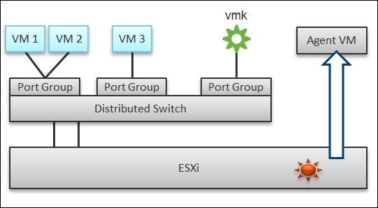
A simplified setup of an ESXi
In a single ESXi host, there are four areas that need to be monitored for complete network monitoring:
- VM network
- The vmkernel network
- ESXi kernel modules
- Agent VMs
In the preceding example, we have three VMs running in the host. VM 1 and VM 2 are connected to the same Virtual Extensible LAN (VXLAN or VLAN). VM 3 is on a different VXLAN, hence it is on a different port group. Monitoring at the Port Group level complements monitoring at the VM level and ESXi level.
Traffic at the Distributed Switch level is more than VM traffic. It also carries vmkernel traffic, such as vMotion and VSAN. Both the vmkernel and VM networks tend to share the same physical uplinks (ESXi vmnic). As a result, it's easier to monitor at the Port Group level.
Sounds good so far. What is the limitation to monitoring at the distributed port group level?
The hint is in the word "distributed".
Yes, the data is the aggregate of all the ESXi hosts using that distributed port group!
By default, VM 1 and VM 2 can talk to each other. The traffic will not leave the ESXi. Network monitoring tools that are not aware of this will miss it. Traffic from VM 3 can also reach VM 1 or VM 2 if an NSX Distributed Logical Router is in place. It is a vmkernel module, just like the NSX Distributed Firewall. As a result, monitoring these kernel modules, and the host overall performance, becomes an integral part of network monitoring.
The fourth area we need to monitor is Agent VMs. An Agent VM is mapped to one ESXi host. It does not need HA protection as every ESXi host has one. It also does not need to reside on a network datastore.
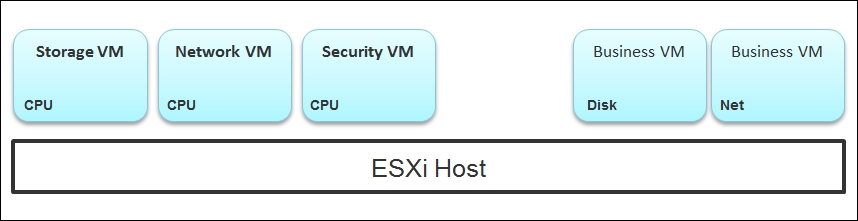
An ESXi Host, Agent VMs, and Business VMs
The diagram shows an ESXi host with three agent VMs. The first VM provides a storage service (an example is Nutanix Controller VM (CVM)), the second VM provides the Network service, and the third VM provides a Security VM.
Let's use the Security service as an example. A popular example here is the Trend Micro Deep Security virtual appliance. It is in the data path. If the business VMs are accessing files on a fileserver on another network, the files have to be checked by the security virtual appliance first. If the agent VM is slow (and it could be due to factors that are not network-related), it will look like a network or storage issue as far as the business VMs are concerned. The business VMs do not know that their files have been intercepted for security clearance, as it is not done at the network level. It is done at the hypervisor level.
A complete monitoring of the network requires you to get the data from five different sources, not just from vSphere. In SDDC, you should also get data from the application, Guest OS, NSX, and NetFlow/sFlow/IPFIX from VDS and physical network devices. For VDI, you need to get data at the application level. I have seen dropped packets at the application layer (PCoIP) when Windows sees no dropped packets. The reason is that the packet arrives out of order and hence is unusable from a PCoIP viewpoint.
The following diagram shows a simplified stack. It shows the five sources of data and the four tools to get the data. It includes a Physical Switch as we can no longer ignore the physical network once we move from just vSphere to complete SDDC.
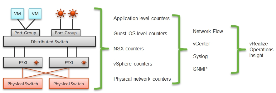
From source to dashboard
Network packet analysis has two main approaches: header analysis and full-packet analysis. Header analysis is certainly much lighter but lacks the depth of full analysis. You use this to provide overall visibility as it does not impose a heavy load on your environment.
vRealize Operations and Log Insight, when coupled with Blue Medora and NetFlow Logic solutions, provides visibility into the physical network and virtual network (NSX).
The impact of virtualization on network monitoring goes beyond what we have covered. Let's add NSX Edge to the mix so that you can see the traffic flow when the edge services are also virtualized. You will see that a network problem experienced by a VM on ESXi A could be caused by another VM running on ESXi B. The following diagram is a simplified setup, showing a single NSX Edge VM residing in another cluster:
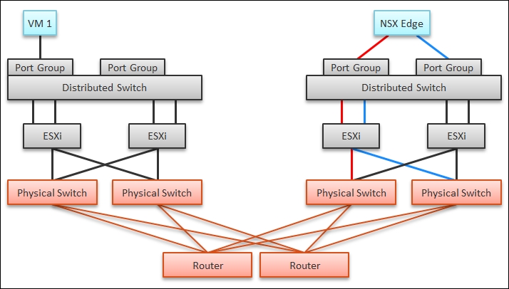
Routing with NSX Edge on a dedicated cluster
In the previous example, let's say VM 1 needs to talk to the outside world. An NSX Edge VM provides that connectivity, so every TCP/IP packet has to go through it. The Edge VM has two virtual NICs, one for each network. If the NSX Edge VM has a CPU issue or the underlying ESXi has a RAM issue, it can impact the network performance of VM 1.
You may be wondering whether an Edge VM does a lot of processing. Let's look at a real-world example. How much traffic do you think this Edge VM is handling?
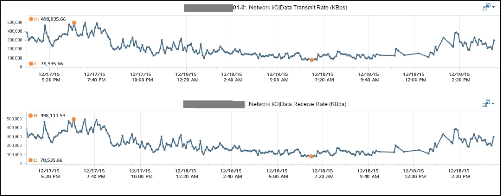
Example of a busy NSX Edge VM
At near 1 million KBPS, the VM is driving nearly eight Gbps' worth of data! This number is the sum of Receive and Transmit, so the theoretical limit is 20 Gbps as this VM uses a 10-Gbps NIC. Notice that the pattern for both Receive and Transmit is identical, as NSX Edge is practically a gateway.
This NSX Edge happens to be the only VM on the host. This means we can expect the data at the host level to mimic that. The host does not run distributed storage (for example, VSAN), so there is no traffic other than this VM. The chart in the following figure confirms this:
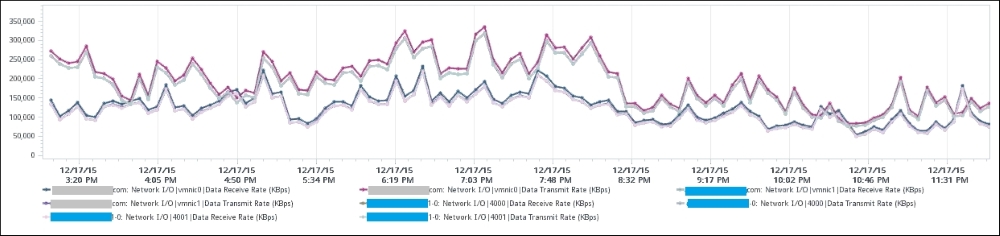
Network utilization at the Edge and ESXi levels
There are practically two lines, even though we've actually plotted eight line charts. What do the two lines map to?
Yes, they map to North-South and South-North traffic. An end user requesting data from a web server would be South-North, while the web server's response would be North-South.
"Wait," you might say, "there should only be four lines! Why do we have eight lines?"
Can you figure it out from the following diagram?
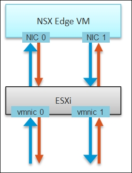
Traffic paths from ESXi vmnics to NSX Edge and back
These eight arrows map to the eight lines. There is one line chart for every arrow. There are four NICs, and each has receive and transmit.
If you use NSX, there is a good chance that you will have multiple NSX Edge VMs. I have a customer with less than 100 VMs. On the same host, you may also run distributed storage (for example, VSAN), as an Edge cluster is typically isolated. I have customers with multiple Edge VMs, and monitoring the health of those Edge VMs becomes an integral part of network monitoring.
vSphere does not provide protocol analysis functionality, which is instead available through a packet analyzer or sniffer program, such as Wireshark and NetFlow Logic's Netflow Integrator. With vSphere alone, you will not know, for example, which VMs are talking to which VMs, the latency they experience, and what protocols are travelling in your network.
NetFlow Logic has developed products that extend both vRealize Operations and Log Insight. Their products also complement the network monitoring solutions from VMware. We will cover this later on in the book.
Good network management is about understanding the application. In a way, we should treat vCloud Suite as an application. There are now two layers of applications in SDDC:
- Infrastructure applications (for example, Virtual SAN, NSX, F5, and Trend Micro)
- Business applications (for example, your company intranet or website)
This is consistent with the fact that you will have two layers of network when it is virtualized. You will use VXLAN for your VM and VLAN for your infrastructure.
When you virtualize your network with NSX, vRealize Operations provides visibility via its management pack for NSX. You can download this complementary product from VMware Solution Exchange at https://solutionexchange.vmware.com.
As of early 2016, most companies have implemented 10 GE technology in their data centers. Network monitoring is both simpler and harder in a 10-Gb environment versus a 1-Gb environment. It is simpler as you have a lot fewer cables and more bandwidth. It is harder as you cannot easily differentiate between traffic types as the physical capacity is now shared.
In 10 GE, you should enable vSphere Network I/O Control (NIOC) because the non-VM network can spike and consume a large bandwidth. The following screenshot shows the default configuration for network I/O control. As you can see, the VM network takes up a small portion. The default value is 100 shares at high priority, with no reservation.
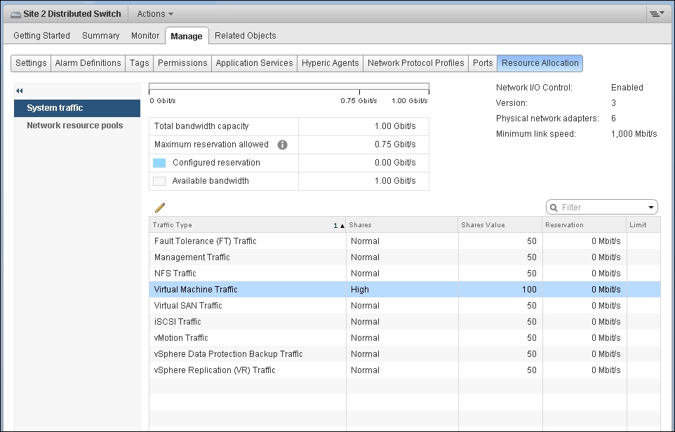
Distributed Switch – the Resource Allocation screen
Relying on load-based teaming to balance the load for performance needs may not provide enough sensitivity to meet SLAs, as it kicks in every 30 seconds. For a discussion about NIOC, review Frank's blog at http://frankdenneman.nl/2013/01/17/a-primer-on-network-io-control and Duncan's blog at http://www.yellow-bricks.com/2013/10/29/virtual-san-network-io-control so that you can configure your settings correctly.
Because the physical capacity of the network is shared, you have a dynamic upper limit for each workload. The VM network port group will have more bandwidth when there is no vMotion happening. Furthermore, each VM has a dynamic upper limit as it shares the VM network port group with other VMs.
In the previous screenshot, we have created a network resource pool and mapped the VM network port group to it. Even if you dedicate a physical NIC to the VM network port group, that NIC is still shared among all the VMs. You do not have a constant number of VMs on a host due to vMotion and DRS, so the upper threshold is dynamic.
The resources available to a VM also vary from host to host. Within the same host, the limit changes as time progresses. Unlike Storage I/O Control (SIOC), NIOC does not provide any counters that tell you that it has capped the bandwidth.
NIOC can help limit the network throughput for a particular workload or VM. If you are using 10 GE, you would want to enable NIOC so that a burst in one network workload does not impact your VM. For example, a mass vMotion operation can saturate the 10-Gb link if you do not implement NIOC. In vCenter 6, there is no counter that tracks when NIOC caps the network throughput. As a result, vRealize Operations will not tell you that NIOC has taken action.
Determining CPU or RAM workload is easy: there is a physical limit. While network has a physical limit, it can be misleading to assume it is available to all VMs all the time.
In some situations, the bandwidth within the ESXi host may not be the smallest pipe between the originating VM and its destination. Within the data center, there could be firewalls, load balancers, routers, and other hops that the packet has to go through. Once it leaves the data center, the WAN and Internet are likely to be a bottleneck. This dynamic nature means every VM has its own practical limit.
Because of this practical consideration, vRealize Operations does not make the assumption that the physical vmnic is the bandwidth available. It is certainly the physical limit, but in most cases, it is not represent the actual bandwidth available. vRealize Operations observes the peak utilized bandwidth and sets this as the upper limit.
The following chart shows that a vCenter 5.5 VM network's usage varies between 18,000 KBPS and 25,772 KBPS during the three days for which the usage has been tracked. vRealize Operations observes the range and sets the maximum network usage to near the peak (25,772 KBPS). This counter is useful in that it tells you that the utilization never exceeds this amount.
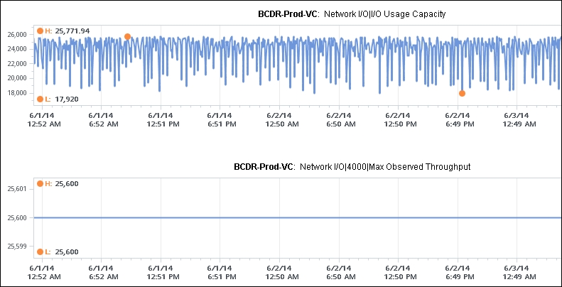
The network workload counter
The Max Observed Throughput number is adjusted dynamically. The following screenshot shows two ESXi hosts in the same cluster. The spike could be due to a mass vMotion in that cluster.
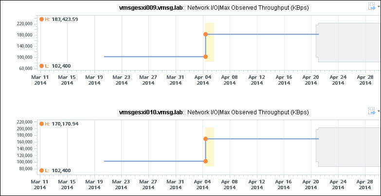
The ESXi network Max Observed Throughput
vRealize Operations does not track the vmnic speed at the individual vmnic level since that's considered a configuration element. It can track at the aggregate level only. Because you normally set the network to auto negotiate, the speed can sometimes drop (for example, from 1 Gbps to 100 Mbps). This is something you need to check manually if you encounter network slowness while your network utilization is below 100 Mbps. In this case, the Max Observed counter can give a clue.
Based on all the preceding factors, the Max Observed counter is a more practical indicator of the network resources available to a VM than the physical configuration of the ESXi vmnic. You should use this counter as your VM maximum bandwidth. For ESXi, you should also use the physical vmnic as a guideline.
vRealize Operations provides the Workload (in percent) counter or Demand (in percent) counter, which are based on this maximum observed value. For example, if the VM Usage counter shows 100 KBPS, and Max Observed Throughput shows 200 KBPS, then the Demand (in percent) counter will be at 50 percent.