
3
Wave Propagation in Structures
3.1 Introduction
In comparison with the wave motion in structures the acoustic wave motion is simple. The equations are isotropic, the speed of sound is (in most cases) not dependent on frequency, and even for complex shapes the Green’s function provides a powerful tool to calculate the wave field. For structural waves the situation is different. In structures there is a variety of wave types described by displacements and rotations in several space dimensions or degrees of freedom. The chance to find a practicable analytical solution is low and solutions are only available for simple systems like straight bars, rectangular thin plates, or membranes. Thus, wave propagation in structures is a natural field for numerics: i.e. finite element methods (FEM) that discretize the real system into many small and simple elements that have an analytical solution or at least an approximation. The dynamics of the full system or the full mesh are defined by the complete set of all these elements.
This book is not about FEM, but we will often use a discrete form of the equation of motion or wave equation. There are two reasons for this:
Complex systems The easiest way to describe the dynamics of a realistic technical system is by numerical methods; thus, there will always by a matrix description of the deterministic system. This is a standard approach in the industrial simulation of structural dynamics.
Formulation There are many ways to describe dynamic wave coupling of different systems, but the discrete formulation is simple, structured, and straightforward.
The various theories to derive the discrete equation are described for example by Bathe (1982). However, the result of this dicretisation process – the matrix presentation of complex structures – will be frequently used. The global structure of the matrices is the same as described in section 1.4 or in Equation (1.89).
There is a large amount of literature dealing with technical mechanics and the statics and dynamics of solid systems. The following deductions are taken from Szabo’s text books Szabo (2013a), (.2013b)or from Lerch and Landes (2012) who used the reference from Cremer et al. (2005). This chapter can only summarize these studies in such a way that the concepts of wave propagation in typical structural systems can be applied for the wave field descriptions in later chapters. Please refer to those publications if more details are required for specific dynamic systems. In order to clarify the principle behavior of waves in representative structures we deal with the wave equations in structures like bars, beams, plates, shells, membranes, and the bulk material. Even if there are not many solutions for real systems available these equations will form the base for all random modelling approaches and provide understanding of the specific characteristics of wave propagation.
3.2 Basic Equations and Definitions
In fluids the state variable of the wave equation was the pressure. In solids there is a similar quantity but with different sign and spatial dependence: the stress. Let us imagine a small block of isotropic material as shown in Figure 3.1. The left hand side depicts a force Fz that pulls a perfectly stiff area connection on top of the block. The force per area is called stress. The nomenclature is such that positive stress is related to an elongation of the block. The normal stress σzz defines the force in the z-direction pulling at the free surface A in the direction normal to it.
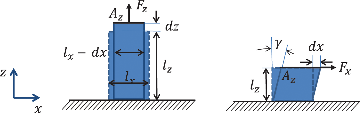
Figure 3.1 Strain and shear of a small solid block. Source: Alexander Peiffer.
We use double indices zz because both the force and the normal vector of the surface point in the z-direction. The ratio of the elongation dz to the unloaded length lz is called the strain in z-direction
The relationship between the stress and strain defines the Young’s modulus E with
The stretching in z is accompanied by a contraction perpendicular to it. The Poisson ratio νxz is defined as the ratio between the strain orthogonal to the stretching e.g. x and the strain in the direction of the elongation..
The surface of the block from Figure 3.1 on the right hand side can alternatively be loaded by a force Fx transverse to the surface normal of Az. This transversal or shear stress is often denoted by τ instead of σ. We stay with σ for all stresses
This shear stress leads to a shear strain γ
The shear modulus is defined as the ratio between the shear strain and shear stress
In this chapter, we will further derive the elastodynamic theory and the related vector conventions to describe the solid wave motion in three-dimensional space.
The displacement d of a point is defined by its coordinates in the three-dimensional space and its displacement components related to a system of unit vectors ex, ey and ez.
 (3.8)
(3.8)A point located at that is displaced by will be located at . In fluid dynamics this would correspond to the Lagrange description (chapter 2). There, the control volume is fixed and the mass and impulse flow are balanced based on this volume. In solid mechanics flow does not occur and we may assume small displacements, e.g. , and stay with the space-fixed convention.
3.2.1 Mechanical Strain
We consider a thin layer of thickness dx in the yz-plane. The displacement of the left point of position x is u. But the displacement of the right point originally located at x + dx is determined by . Thus the strain in the x-direction is given by:
A similar relationship can be found for y and z-directions.
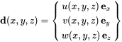
The deformation of a solid can be described by the superposition of the following particular deformations:
- or global volume change into the orthogonal dimensions of space, i.e. strain in ɛii in dimension . (Figure 3.3a)
- deformation with angle . (Figure 3.3b)
- or rigid body motion with rotation angle βi with i being the normal vector to the plane of rotation. (Figure 3.3c)
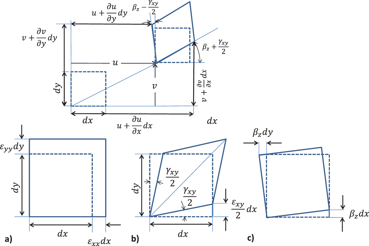
Figure 3.3 Deformation of a two-dimensional element of edge length dx and dy. Source: Alexander Peiffer.
Figure 3.2 One dimensional displacement and strain of a thin layer of thickness dx. Source: Alexander Peiffer.
With those considerations we get the relationship between the shear angle and the rotation angle β to the mechanical displacement. Assuming very small angles so that this leads to
The difference of equations (3.12) and (3.13) gives
and the sum of both equations leads to an expression for the deformation angle
A similar expression can be found for the other shear angles ɛyz and ɛzx
3.2.1.1 Mechanical Strain - Voigt Notation
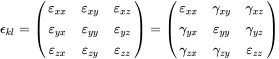
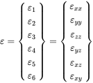
The mechanical strain ɛij in three-dimensional space is the relative displacement of component i along dimension j. This is given by a symmetrical tensor of second order
 (3.18)
We separate out the normal strain in the diagonal ɛii that is defined as the extension into dimension i related to unit length. The shear strain is given be the shearing angle . Thus we can define for , and
Due to its symmetry the tensor in equation 3.18 has only six independent components, so the tensor can be alternatively represented in theVoigt notation
 (3.20)
3.2.1.2 Dilatation dilation – Relative Change in Volume
The relative change of a volume can be found from the linear strains:
3.2.2 Mechanical Stress
According to the introduction of this section every force vector can be separated into two components (Figure 3.4):
- normal stress: A normal force Fn in the direction of the normal vector of the surface.
- shear stress: A tangential force perpendicular to the normal vector.
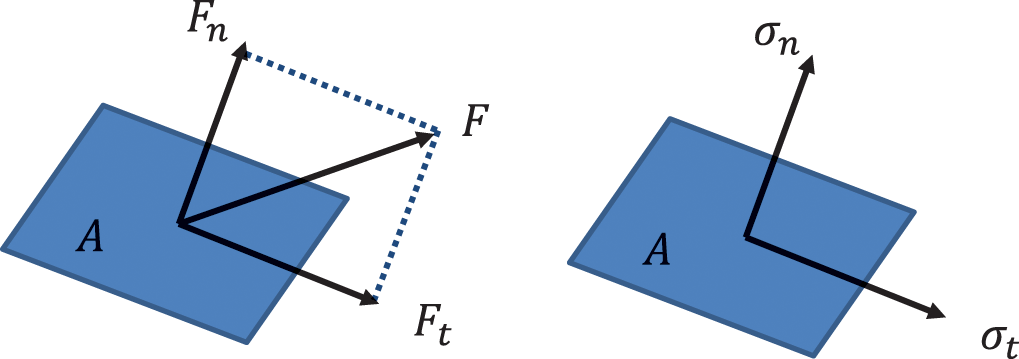
Figure 3.4 Force and unit area A. Source: Alexander Peiffer.
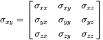
We consider the surfaces of a cube as shown in Figure 3.5 with the axes parallel to the coordinate axes. The symbol for stress is σ; the first index denotes the direction normal vector, and the second index the direction of the force. Thus, σxx, σyy and σzz are the normal stresses. σij with and are the shear stresses. The definition is

Figure 3.5 Stresses at the surfaces of a control volume Source: Alexander Peiffer.
Because of the moment of equilibrium the stresses of exchanged indices must be equal
Finally σij is a symmetric tensor of second order.
 (3.24)
So we have six independent components of the stress tensor, and we can apply the Voigt notation
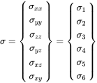 (3.25)
3.2.3 Material Laws
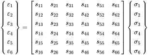
The relationship between the strain and stress tensors is given by the material laws called Hooke’s law for linear elastic media. These laws in their most common form are given by:
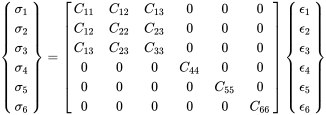
The first tensor is called the stiffness tensor or elasticity tensor and the second is named compliance tensor. They have 81 components that can be reduced to 36 because of symmetry. Using the Voigt notation the stress tensor can be written as a matrix
 (3.28)
Those complex notations and equations are fortunately not that often necessary. For most engineering applications two special cases are applied: (1) Isotropic material, for example (steel, rubber, aluminium) and (2) orthotropic material (carbon fibre reinforced plastic (CFRP), steel enforced concrete, wood, plywood, etc.)
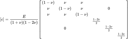
3.2.3.1 Isotropic Materials
Isotropy means, there is no dependency of the Hooke’s law on space dimension or orientation. For the normal stress in the x-direction (or any other) we have
This behavior is valid if the solid may perform lateral contraction. That means the elongation of a rod leads to lateral contraction. If this contraction is not constrained by surrounding solid material the elongation is reduced by the Poisson ratio ν, the negative ratio of transverse motion to axial strain. The strain due to stress in one direction must be corrected by the strain from other normal directions and the Poisson number.
We can also apply shear stresses. There is a similar relationship to Equation (3.29)
Those three material constants are not independent, and they are linked by
Summarising all properties we can write the compliance and stiffness matrices:
 (3.35)
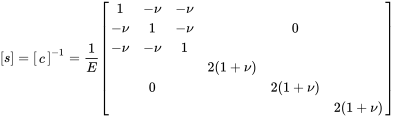 (3.36)
3.2.3.2 Ortotropic Solids
This class of material occurs for example in composites with fibres or layered microstructures. The properties change with the normal axes of the three-dimensional coordinate system. Thus, orthotropic materials have three orthogonal planes of symmetry. If they coincide with the coordinate system we get for the stiffness matrix a common notation.
 (3.37)
This matrix can be derived from the inversion of the compliance matrix. However, this leads to lengthy expressions that will not provide any additional insight, whereas the compliance matrix can be presented in a compact form
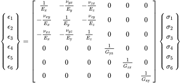 (3.38)
where is the Young’s modulus along axis i, Gij is the shear modulus in direction j on the plane whose normal is in direction i. νij, is the Poisson’s ratio that corresponds to a contraction in direction j when an extension is applied in direction i.
3.3 Wave Equation
In solids there are several modes of wave propagation. In addition the type of wave mode depends on the structure geometry, if it is infinite bulk material, a flat or curved plate, a beam or rod. In the following sections we will go step by step through the different wave equations for several structural configurations. For fluids the wave equation was derived from the linearized versions of the equation of motion or Newton’s law and a combination of the continuity equations and the state law. For solids the wave equation is determined from the equations of motion and the material laws. In this section we will only deal with isotropic materials.
3.3.1 The One-dimensional Wave Equation
The field quantity for solids is the displacement . We start from the control volume as shown in Figure 3.5. If we assume a cut-free cube there is a stress balance at each cube surface: i.e. that the stresses are in balance at each interface and have opposite direction (Figure 3.6). From the stress balance over the cube surfaces the resultant force in the x-direction is:
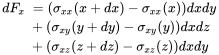 (3.39)
Figure 3.6 Stresses at the surfaces of a control volume (top view) Source: Alexander Peiffer.
From Newton’s law and with we get after division with and the series expansion for
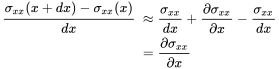 (3.40)
the equation of motion in the x-direction
Similar treatment leads to the two equations of motion in y and z-directions
Thus, for deriving the wave equation in displacement coordinates the stresses must be expressed in terms of the displacement making use of the stress–strain relationship of isotropic solids. We start with the sum of equations (3.30)–(3.32).
With the definition of the dilatation (3.21) and (3.34) this gives:
The goal is to find an expression for σxx depending only on displacements not linked to other stresses. We start with (3.30) solving for σxx and adding on both sides.
With (3.45) this leads to
Eliminating E yields
or
We introduce the Lamé constants
λ is a measure for the extension perpendicular to the stress. Applying these constants we get from (3.50)
The equations for the y and z-directions can be derived similarly:
From the definition of the isotropic shear modulus (3.33) and the shear strains (3.15) the equations for the other components are found:
Using equations (3.53)–(3.58) we get after some algebraic modifications the wave equation for the one-dimensional case in the x-direction
Similar and equivalent derivation can be done for the remaining two dimensions.
3.3.2 The Three-dimensional Wave Equation
Collecting the one-dimensional wave equations and putting them together for the displacement vector d leads to
With the identity we get the wave equation in a different form
This wave equation can only be solved in closed form for simple geometries. In most cases numerical methods like the finite element method must be applied to solve this equation for realistic systems.
There are two differential operators in space on the LHS of Equation (3.63) indicating two wave types in solids. Any vector field can be separated into two independent components. The irrotational and the source-free or zero-divergence component
An irrotational field is characterized by
and a source free field by
Thus
These relationships show that there are two independent wave types in solids, called longitudinal waves (L) and shear or transversal waves (S).
3.4 Waves in Infinite Solids
In order to understand the principle dynamics of both waves we consider an unbounded infinite solid. Practical applications can be found in geophysics or ultrasonics for non-destructive testing. Engineering acoustics and vibroacoustics usually deal with vehicles. Thus, the construction must be lightweight, and bulky solid materials are rarely found. With one exception, some materials for acoustic treatment such as foams have soft bulk material with wavelengths small enough that those wave types occur in practical technical systems.
3.4.1 Longitudinal Waves
Longitudinal waves are rotation free, thus and the wave equation (3.63) simplifies to
cL is called the longitudinal wave speed. In isotropic materials this is the wave with the highest speed. When we calculate cL for typical materials like iron, aluminium, wood etc., it becomes obvious why the practical relevance in vibroacoustics is quite low. For example, for iron the wavelength at f = 1 kHz equals 5 m, extending by far beyond the typical dimension of bulk parts in a car. In order to illustrate the propagation of a longitudinal wave we calculate the solution for propagation into the x-direction. That means and . The longitudinal wave equation reduces to
The wave motion is characterized by particles oscillating in the direction of propagation. All shear stresses are zero, and a plane of constant dilatation propagates in the wave direction. Thus, those waves are also called dilatation or density waves. Equation (2.34) from chapter 2 can be applied, and the harmonic solution is
In the upper part of Figure 3.7 the particle motion is shown for this wave type.

Figure 3.7 Displacement of solid particles for the different wave types. Source: Alexander Peiffer.
3.4.2 Shear waves
In contrast to the longitudinal wave the shear wave is source free, thus . In that case the wave Equation (3.63) leads to
The wave motion is iso-voluminous. It can be shown by the introduction of a rotation vector that the particle motion is orthogonal or transversal to the wave propagation (Graff, 1991). This is the reason why this wave type is also called transversal wave. A simple plane wave equation for w is
A solution in the positive x-direction is for example
In the lower part of Figure 3.7 the particle motion for one fixed time is shown. From (3.34) it follows that shear waves are slower than longitudinal waves.

Figure 3.8 Beam in x-direction with cross section A. Source: Alexander Peiffer.
3.5 Beams
Beams are one-dimensional structures that have a cross section small compared to their length. Due to the large wavelength derived for the bulk material we can assume that there is no wave propagation perpendicular to the main axis of the beam. There are a variety of wave types, but we will deal only with two in this section.
3.5.1 Longitudinal Waves
Longitudinal waves are associated with normal stresses in the direction of the beam axis. We consider a free cut small layer of the beam and take the stress balance (3.32). There are no constraints for y and z surfaces and therefore . Thus, the stress strain relationship in the x-direction reads
Using this we get with Newton’s law from Equation (3.41)
or in harmonic form for
The solution of this one-dimensional wave equation is
Due to the fact that the bar is stress free in the direction normal to the bar axis, the wave speed in bars cLB is slower than the longitudinal wave speed in infinite solids. This lead to displacement in y and z that can be calculated from the first column of (3.36):
The only information related to the cross section that is required for the determination of the longitudinal wave speed is that the dimensions of the cross sections must be small compared to the wave length.
3.5.2 Power, Energy, and Impedance
When exciting a half beam as shown in Figure 3.9 we create a wave propagating in the positive direction leaving out the e−jkx from (3.78)

Figure 3.9 Excitation of longitudinal waves in half infinite beam. Source: Alexander Peiffer.
The stress in x is with (3.75):
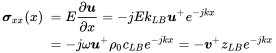 (3.82)
So, there is a longitudinal characteristic impedance of the longitudinal wave in beams. Assuming a force Fx exciting the beam in the x-direction via a stiff plate at the beam cross section leads to the boundary condition at x = 0 with
The mechanical impedance follows from this
The power introduced into the system is, when we assume without loss of generality
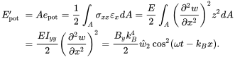
This power propagates into the beam and creates an energy density per length , because the power per time unit is distributed with velocity cLB over the related length unit. This can also be proven in a more complicated way by deriving the kinetic and potential energy density per length
For the potential energy we have to integrate the stress over the strain
with we get for the potential energy density per length
So we find . With (3.83) we get for the total energy expressed for the velocity
Integrating over one wavelength λ gives the total length specific energy
proving the above arguments regarding power and speed of sound.

Figure 3.10 Various quantities for longitudinal wave propagation in structures. Source: Alexander Peiffer.
3.5.3 Bending Waves
The bending stiffness depends on area and shape of the cross section. In Figure 3.11 the cross section, forces, and moments of a cut-free slice of the beam are shown. We assume that there is a neutral axis without any dilation and pure bending. That means that each cross section of the un-loaded straight beam remains orthogonal to the neutral axis as shown in Figure 3.12. This is called the Bernoulli assumption.
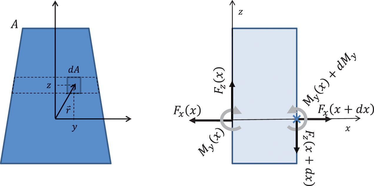
Figure 3.11 Cross section and segment of a beam. Source: Alexander Peiffer.

Figure 3.12 Bernoulli bending of beams. Source: Alexander Peiffer.
Geometrically this assumption means that all fibres stay orthogonal to the cross section. The stress is linear with the bending radius R as depicted in Figure 3.12. The stress in the direction of the neutral axis vanishes at the neutral axis1. The strain out of the neutral axis can be derived from Figure 3.12.
and therefore
Due to Equation (3.29) it can be shown, that the stress is a linear function of the distance from the neutral axis z and the curvature .
The moment vector is given by the integral over all small moment contributions at r with . Thus:
and due to the assumptions the stress is symmetrical to the z-plane
We call
the second moment of area, in most literature called moment of inertia2. The moment
that vanishes in our special case is called the product moment of area. There are axes of the cross section where this product moment is zero. They are called the main axes and are for example the symmetry axes of a symmetrical section. Using (3.94) we can write (3.92) as
Using the following differential equation for the curvature
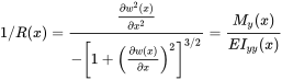 (3.97)
We assume small displacements , and we get approximately
and with that
For the z-axis we get accordingly
The force in the z-direction can be derived from the moment equilibrium at the position x + dx in Figure 3.11.
Now, we set up the force balance at the control segment from Figure 3.11.
Performing the limiting process for dx → 0 gives
with mʹ being the mass per length or length specific density. The prime specifies units per length in this section. Using the harmonic wave solution we get the bending wave equation in the frequency domain
with the beam bending stiffness and for the principle y and z-axes of the cross section. Neglecting the time dependence and performing the spatial derivatives we get for the bending wavenumber
with two real and two complex solutions
Thus the solution includes two propagating waves and two decaying
We neglect the complex wave numbers leading to exponential decaying waves and calculate the wave speed from the fourth root of (3.105)
Here, we have the effect of dispersion, and the wave speed depends on the frequency. The main effect is that the propagation of energy is different from the propagation of constant phase in the wave. This was not the case for fluids where the speed of sound is constant over frequency. The consequences of this will be discussed in section 3.8.
If we calculate the bending wave speed for a typical system we see that we have a wave speed of similar order of magnitude as in air. Let us consider a rectangular cross section as shown in Figure 3.13. The moments are

Figure 3.13 Rectangular cross section. Source: Alexander Peiffer.
Assuming aluminium with isotropic material properties Pa, kg/m3 and ν = 0.34 the rectangular cross section with and yields the following wave speed for bending in the z and y-directions (Figure 3.14).

Figure 3.14 Bending wave speed of rectangular aluminium beam (b = 3 cm,h = 2 cm). Source: Alexander Peiffer.
3.5.4 Power, Energy, and Impedance
The frequency dependence of the wave speed leads to a different propagation speed, point of constant phase, and energy stored in the wave. For the power considerations we summarize the following relationships from the above calculations
One power component in beams is the force–velocity product as in (1.47). In addition the product of moment My and the rotational speed must be taken into consideration
with
We keep the oscillating part of the power in order to show a characteristic effect for wave propagation in beams. We will use the positively propagating part of the harmonic solution (3.107) and neglect the evanescent wave that is not relevant for power transport. For further simplifications of the expressions we assume a real displacement amplitude and we get for the force and the velocity
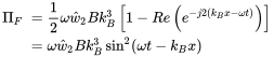 (3.116)
Force and velocity are in phase and the same is true for moment and rotational velocity, but with a phase shift of
 (3.119)
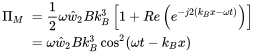
Thus, both contributions sum up to the constant value
The same must be true for the energy. If we multiply the kinetic energy density ekin by the beam area we get for the translational energy per length
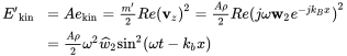 (3.121)
The rotational component can be neglected, as we can see from
 (3.122)
The averaged ratio between both kinetic energies is
 (3.123)
The so called radius of gyration is the perpendicular position of a point mass which gives the same rotational inertia. As we stated in the beginning, one main assumption was that the cross sectional dimensions must be small compared to the wavelength λB. Consequently we can neglect the rotational part of the energy, too.
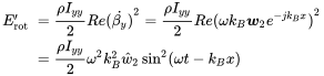
Due to the Bernoulli assumption only in-plane stress and strain must be considered. Here the stress and strain in the x-direction. Therefore, the potential energy per length is given by
 (3.124)
Figure 3.15 Various quantities for bending wave propagation in beams. Source: Alexander Peiffer.
Both kinds of energy oscillate between 0 and the maximum value similar to the power. Using the dispersion relation (3.105) the sum of both gives
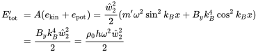 (3.125)
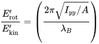
So, we have a constant energy distribution in the wave. There is no energy oscillation as was the case for fluid waves. If we relate the power transport (3.120) to the above energy we get
The power transportation is given by twice the phase speed cB, which is fine in this case, because the uniform distribution of power and energy allows this effect. This is not an error and comes from the dispersion of the bending waves as we will see in section 3.8. The power transport in dispersive media is not given by the phase velocity but by the group velocity for bending waves in beams.
A force exciting the beam radiates waves into the beam. In order to describe the source performance we come back to our impedance concept. As the force shall excite waves in the direction the bending occurs we apply a harmonic force in the z-direction.
We start with a half infinite beam that is excited at x = 0, Figure 3.16. From the boundary condition it follows that as it is an open end. From the origin only waves that propagate in the positive x-direction occur. Thus, we use the following part of Equation (3.107)

Figure 3.16 Force exciting a half infinite (top) and infinite beam at x = 0. Source: Alexander Peiffer.
So we get for for My and Fz
At x = 0 the first condition leads to and with this we get for the second equation balancing the force :
and hence
For the mechanical impedance at x = 0 we get now:
For the infinite beam we assume a mirrored wave at x = 0 propagating away from the point of excitation, but now the moment does not need to be zero. For symmetry reasons the the rotation βy must vanish at the exciting force position. Thus, with Equation (3.16) used in the y-direction and vanishing displacement the condition is
The force is now driving two half beams, thus
and
This gives for the impedance of the full beam:
The full beam impedance is four times higher than the impedance of the half infinite beam. With growing frequency the impedance decreases, but we must keep in mind that for higher frequencies the Bernoulli beam assumptions are no longer valid. The impedance is complex with a phase of . The driving force experiences a reactive and a resistive part. In Figure 3.17 three time or phase slots of an infinite and half infinite beam excited by a force are shown in combination with the solution without the evanescent part. We see that this part contributes only to the near field at the point of excitation and therefore contributes only to the impedance.

Figure 3.17 Beam displacement w for certain phases (). The dotted line is without the evanescent part e−kx. Source: Alexander Peiffer.
3.6 Membranes
Membranes don’t have an inert bending stiffness from their mechanical properties. The stiffness comes solely from the tension Tmem in the membrane. Though membranes don’t occur frequently in technical systems, it helps predefining the effect of pressurisation in a closed cabin, e.g. in an aircraft. The pressurisation leads to an additional bending stiffness coming from the tension.
If a small plate in the xy-plane is displaced in the z-direction by w the force due to the tension per length is only determined by the slope θ of the membrane as shown in Figure 3.18. For small displacement w we get for the force per length in the z-direction acting on the membrane element edge of length dy

Figure 3.18 Membrane forces in the x-direction. Source: Alexander Peiffer.
The total force from tension acting on a membrane element along dy and due to the slope in x is
Using the similar equation in the y-direction we get with Newton’s law the membrane wave equation
Here, mʹʹ is the mass per area for the membrane, and we have assumed . The membrane wave equation does not have any dispersion effects. This is the reason why drums should be made from membranes and not plates. Plates have dispersion effects as with beams, and this does not allow the wanted multiple harmonics as desired for musical instruments.
3.7 Plates
The theory of thin plates is summarized here according to Ventsel and Krauthammer (2001). The usual nomenclature distinguishes between plates that are flat, and thin structures and shells that can be curved. In terms of technical relevance plates and shells are the most important structure in many vibroacoustic investigations. Plates provide high stiffness at low weight. Thus, most means of transportation vehicles are created by enclosures made of plates and shells. For example the body of a car is made out of several sheets of steel that are stamped and point welded. The following assumptions for thin plates are made:
- The plate is thin: the thickness h is much smaller than the other physical dimensions.
- The in-plain strains are small compared to unity.
- Transverse shear strains ɛxz and ɛyz are negligible.
- Tangential displacements u and v are linear functions of the z coordinate.
- The transverse shear stresses vanish at the surfaces at ().
3.7.1 Strain–displacement Relations
Using the fourth assumption the tangential displacements are of the form
u0 and v0 are the tangential displacements of the middle plane. Entering these equations into the related strain–displacement relationships (3.16) and (3.17) and using assumption three yields
Therefore.
This result is illustrated in Figure 3.19 for a pure bending configuration.

Figure 3.19 Deformation of a small plate element in the xz-plane. Source: Alexander Peiffer.
The strain displacement relation (3.19) leads to
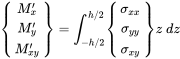
We consider an infinitesimally and cut-free small plate element as shown in figure 3.20. For the plate dynamics it is convenient to integrate over the plate thickness to get quantities defined per length instead of area. The integration over the normal stresses reads:
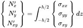 (3.148)
Figure 3.20 Plate element with stresses on the free faces. Source: Alexander Peiffer.
3.7.2 In-plane Wave Equation
From Figure 3.19 it becomes obvious that the bending is decoupled from the in-plane motion of shear and stress in case of homogeneous thin plates. Bending leads to symmetric stress and strain, and the integrals in Equation (3.148) are thus decoupled from the in-plane motion.
From assumption five it follows that the strains ɛx and ɛy can be given according to equations (3.30) and (3.31)
With the above equations and component xy in Voigt notation from (3.33) corresponding to the xy index in (3.19) we get
Entering equations (3.151)–(3.153) into (3.148) provides
because the last term in Equation (3.145) vanishes due to symmetry. We get for and accordingly
In Figure 3.21 the force balance of a plate element is shown. The balance in the x-direction is
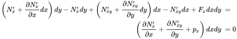 (3.157)
Figure 3.21 In-plane stress and shear force balance of cut-free plate element. Source: Alexander Peiffer.
Division by area dxdy gives
and accordingly for the y-direction
With (3.154)–(3.156) we get finally, setting and :
 (3.160)
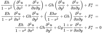
Equalising the force per area to the external pressure plus inertia forces and using
leads to the wave equation for in-plane waves. Together with the following abbreviations
we get
and in a similar way for the y-direction:
The motion in the in-plane direction is coupled: a displacement in u leads to motion in v and vice versa. The solution of both equations leads to two waves analogical to the longitudinal and shear waves of the solid material in section 3.4.
3.7.3 Longitudinal Waves
In longitudinal waves the wave motion is in the direction of propagation. Without loss of generality we choose the x-direction as propagation direction. Thus, there is no change of u over y and v is zero.
Using these assumptions in (3.163) we get
and the wavenumber yields
We see that this third longitudinal wave speed for plates is valued between the solution for the longitudinal waves in solids and beams.
The more constrained the bulk material is the stiffer it becomes due to the lateral contraction. The strain in thickness can be calculated from (3.32).
Integrating the strain over the thickness delivers the shape of the wave motion.

Figure 3.22 Shape of longitudinal wave in plate. Source: Alexander Peiffer.
3.7.4 Shear Waves
Shear waves have displacement perpendicular to their direction of propagation. For shear wave propagation in the x-direction we assume:
Using (3.164) with these conditions gives the shear wave equation in the x-direction for plates:
The shear wave speed in plates or solid material is similar, because this wave type is free of dilatation due to condition 3.169 and thus not dependent on geometrical constraints.
3.7.5 Combination of Longitudinal and Shear Waves
The combined dynamics of in-plane wave motion is found by entering the ansatz
with being the index for both wave types. Entering this into (3.163) and (3.164) leads to the following system of equations
We used following from (3.167) and (3.171). Equation (3.174) can be seen as a generalized eigenvalue problem with eigenvalue . Dividing the above equation by S leads to a form that is more practical for the next steps
With the relationship
This can be further modified to
For non-trivial solutions of this matrix the determinant must vanish, and this leads to the equation
This is of the form . So the two solutions are
using relationship (3.176) again. Finally, we have derived the above wavenumbers for shear and longitudinal waves in a more formal way. Entering and for into (3.177) provides the solution for the shape of the wave propagation. With we get:
So , and when we choose we get ; finally the displacement due to the shear wave motion is given by
With the same equation reads as:
providing the longitudinal wave motion
The in-plane wave propagation is given by the superposition of both waves with:
The displacement of longitudinal waves is parallel to the propagation direction given by , and the shear wave displacement is perpendicular to the propagation direction orientation kS as shown in Figure 3.23

Figure 3.23 Propagation direction of in-plane waves and orientation of displacement. Source: Alexander Peiffer.
Similar to solids the wavelengths of longitudinal and transversal waves are very high. Thus, in-plane waves can be neglected in many technical acoustics problems at audible frequency, but they are required for a full understanding of the physics when plates are coupled.
3.7.6 Bending Wave Equation
For the derivation of the bending wave dynamics we define the moments per length Mʹ parallel to the edges and as a torsional moment.
 (3.185)
The thickness integration over the shear stresses gives the shear forces per length:
With those definitions and according to Figure 3.24 we can now set up the relationships for the required equilibrium of the total forces in the z-direction

Figure 3.24 Moments and shear forces balance of cut-free plate element. Source: Alexander Peiffer.
and for the moments around the x-axis,
and the y-axis accordingly:
Neglecting terms of second order and with the moment equilibrium we get
Entering and from (3.188) in (3.191) gives
As mentioned above the bending motion is decoupled from the in-plane motion. So, we assume and get with (3.145) for the displacement in the thin layer an approximately linear dependency from z
Entering (3.193) into (3.151)-(3.153) leads to the in-plane stresses as function of w and z
This is applied in the definitions (3.185) and reads for
with the bending stiffness B of the plate
With equations (3.191) and (3.197)–(3.199) the shear forces can also be expressed as functions of w .
From (3.192) and with equations (3.197)–(3.199) we can derive the plate equation
In order to get the wave equation for plates we set the force per area equal to external pressure plus the inertia force
Hence.
Now we are prepared to determine the wave speed for bending waves in plates using the solution in frequency domain
Considering waves in the x-direction without loss of generality the results for kB are similar to the results of the beam bending waves
and the wave speed
Equation (3.206) can be written in Helmholtz form
We get again two real and two complex solutions:
Thus the solution includes four propagating waves. Using only the positive absolute values per definition with
we can write for the four waves in the x-direction
The dispersion effects discussed in the beam section are also valid.

Figure 3.25 Shape of bending wave of a plate. Source: Alexander Peiffer.
3.7.6.1 Cylindrical Solution of Bending Wave Equation
In order to derive the mechanical impedance for a plate we must agree on a certain set of boundary conditions and assumptions that allow for a solution:
- The solution is rotationally symmetric.
- The point of excitation is rotation free.
- The solution fulfils the Sommerfeld condition: i.e. that the wave decays in large distances.
Starting with (3.206), using the wavenumber result from (3.207) and rewriting it to
gives the following system of equations:
The first Equation (3.213a) is similar to the Helmholtz equation for fluids but for two dimensions. The solution is the Hankel function of second kind:
With r being the distance from the point of excitation. For the far field properties and the behavior at the excitation point we use the asymptotic behavior for small and large values of x
The solution of the second Equation (3.213b) can be found by replacing kBr with , hence
For large kr we get
Thus, Equation (3.215) represents the exponentially decaying near field, as in (3.106). The total solution is
With the assumption that the rotation
must vanish at r = 0, so that
we finally get
3.7.6.2 Power, Impedance, and Energy
The value at r = 0 follows from the asymptotic expression for small values:
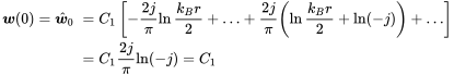 (3.219)
So C1 equals the displacement amplitude at the excitation point.
Some shapes at specific phases of the force are shown in Figure 3.26.

Figure 3.26 Bending wave forms of plate excited by a force Fz at r = 0. Source: Alexander Peiffer.
In order to derive the displacement amplitude we consider a small circle around the the point of excitation and use equations (3.201)–(3.202) in cylindrical coordinates
Entering this into (3.218) leads to:
Using the approximation of the Hankel function for small arguments gives
Multiplication of (3.223) with the perimeter of a small circle finally provides the force

Figure 3.27 Force excitation at a small disc of radius r0. Source: Alexander Peiffer.
Entering this into (3.220) we get the shape of the plate due to force excitation
With the velocity at the centre we get a surprisingly simple expression for the mechanical impedance at r = 0:
Regarding the energy in the plate, we rely on the considerations of bending waves in beams in section 3.5. The property characterising bending for beams was the Young’s modulus times the second moment of area, e.g. . For plates this must be replaced by the bending stiffness that is defined per length as given in equation 3.200. Thus, after adjusting Equation (3.125) to this length reference we get area energy density
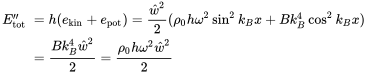 (3.227)
The equality of kinetic and potential energy, as far as the fact that the energy is not pulsating but constant over time, is also similar to beams. The expression for the power flow has to be adjusted to power per length or length intensity with
Note that the energy is transported with twice the phase wave speed, which is not in contradiction to the energy conservation because of the fact that the energy is equally distributed over the phase cycle. For the point force excitation the introduced energy flows through the edge of a circle of radius r with the circumference .
The input power is known through the point impedance (3.226)
Combining equations (3.228) to (3.229) we get an expression for the displacement amplitude derived from energy considerations:
The same expression can be derived from Equation (3.225) when using the asymptotic expression for the Hankel function for .
Damping
The damping of wave propagation is related to energy or the transport of energy. This complicates the treatment for dispersive waves. To overcome this issue we use the damping loss as the complex ratio of stiffness related quantities from (1.62). For plates this is the complex Young’s modulus E:
impacting linearly the bending stiffness:
When we introduce this into Equation (3.207)
and
In contrast to Equation (2.59) this is one-fourth of the wavenumber. The reason for this is that due to dispersion of bending waves the energy propagates twice as fast as the phase.
3.8 Propagation of Energy in Dispersive Waves
The bending wave considerations have shown that the phase velocity does not represent the speed for energy transportation. It is twice the phase wave speed as in Equation (3.126). An illustrative way to present the relationship between group and phase velocity is to investigate the interference of two one-dimensional waves.
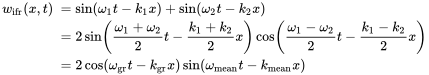 (3.235)
The interference of the two sine waves leads to a carrier wave with mean frequency and wave number whose amplitude is modulated by a much lower frequency and the much lower wavenumber .
The energy in the wave is proportional to the squared amplitude of the wave. Thus, the energy is transported with the speed of the amplitude modulation:
In the limit of the group velocity will be
In Figure 3.28 an example for bending waves is depicted. We see how the envelope propagates with the group velocity cgr. If we follow one phase value of the carrier we would notice that it propagates with a slower speed. This can also be recognized by inspecting the relative location of the carrier in the envelope. The maxima are located at different positions in the envelope.

Figure 3.28 Group and phase velocity of two sine waves with similar frequency. Source: Alexander Peiffer.
We conclude that the speed of energy propagation in waves is the group velocity. If there is no frequency dependence phase and group velocity are the same. We have found this relationship already in the context of power flow for bending waves in beams in Equation (3.126).
The consequence of the fact that energy travels with group velocity is that the relationship between energy density and intensity (2.53) must consider the group velocity.
3.9 Findings
With chapters 2 and 3 we have described several modes of wave propagation with different properties. Those modes are different in terms of sound speed, excitation impedance, and the relationship between energy density and the wave property. In Table 3.1 those properties are summarized.
Table 3.1 Wave speeds of structural waves
| Mode type | Group velocity | Phase velocity |
|---|---|---|
| Longitudinal waves in bars | ||
| Torsional waves in bars | ||
| Bending waves | ||
| Longitudinal waves in plates | ||
| Shear waves | ||
| Waves in elastic solids |
Bibliography
- Klaus-Jürgen Bathe. Finite Element Procedures in Engineering Analysis. Prentice-Hall Civil Engineering and Engineering Mechanics Series. Prentice-Hall, Englewood Cliffs, N.J, 1982. ISBN 978-0-13-317305-5.
- Lothar Cremer, Manfred Heckl, and Björn Petersson. Structure-Borne Sound: Structural Vibrations and Sound Radiation at Audio Frequencies. Springer Verlag, Berlin, Germany, 3rd edition, December 2005. ISBN 978-3-540-26514-6.
- Karl F. Graff. Wave Motion in Elastic Solids. Dover Publications, New York, 1991. ISBN 978-0-486-66745-4.
- Reinhard Lerch and H. Landes. Grundlagen der Technischen Akustik, September 2012.
- I. Szabo. Einführung in Die Technische Mechanik: Nach Vorlesungen. Springer Verlag, Berlin, Germany, 2013a. ISBN 978-3-662-11624-1.
- I. Szabo. Höhere Technische Mechanik: Nach Vorlesungen. Klassiker Der Technik. Springer Verlag, Berlin, Germany, 2013b. ISBN 978-3-642-56795-7.
- Eduard Ventsel and Theodor Krauthammer. Thin Plates and Shells: Theory: Analysis, and Applications. CRC Press, August 2001. ISBN 978-0-8247-0575-6.
Notes
- 1 The direction convention differs from the plate theory. The main reason for that is that the moments are defined in such a way that the curvature for positive moment is also positive
- 2 There are many wordings used for the second moment of area: moment of inertia of plane area, area moment of inertia, or second area moment. There is no mass involved in the definition, so the expression “inertia” might be misleading.