5.1 Introduction

The complex situation of wave propagation in structures becomes even worse for closed structural systems. When specific features like holes, rigs, beading or any complicated shape is given, this is definitely the world of numerical methods. Current finite element methods (FEM) in combination with pre and post processors can handle very complex and large systems as for example trains or aircraft. But, the modelling procedure, the creation of the mesh, and the population of the property and material database are time consuming. Analogous to fluid systems we stay with academic cases to work out the full frequency range.

Even though we are not dealing with the details of FEM we will rely on the discrete representation of systems as introduced in section 1.4. Some of the following treatments rely on the discrete matrix formulation of structures, that is the dynamic stiffness matrix. Thus, the principle definitions are given without description of the finite element method. Please rely for example on the textbook from Bathe (1982) for more details. In Chapter 3 the equations of motion are expressed in displacements $u,v,w$, the components of the stress tensor for the bulk material ${\sigma }_{ij}$ and forces and moments $F_i,M_i$. Rotations ${\beta }_i$ are approximated as the derivative of displacement components.

In finite element theory the rotational components are considered as dedicated degrees of freedom. Thus, in this chapter the natural coordinates will therefore be the displacements $u,v,w$, the rotations ${\beta }_x,{\beta }_y,{\beta }_z$ and the according forces $F_x,F_y,F_z$, and moments $M_x,M_y,M_z$.

Consequently all discrete structural subsystems are described using a dynamic stiffness matrix of the form:

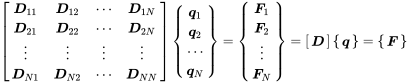  (5.1)

$\left\{\begin{array}{c}\mathit{q}\end{array}\right\}$ is the vector of generalised displacement degrees of freedom including rotations. The vector is called generalised because the displacement can be represented in any base coordinate system, for example modal coordinates, wavelets or wavenumber. Consequently, $\left\{\begin{array}{c}\mathit{F}\end{array}\right\}$ is the generalised force vector including forces and moments of the accompanying displacements.

Due to the fact that the displacement is the natural degree of freedom we switch from the impedance to the dynamic stiffness concept. In the complex notation we may easily change between velocity and displacement using the $j\omega$ factor for the derivative.

However, even if structure systems are very complicated it is necessary to elaborate some solutions for representative systems in order to be prepared for random methods, and the modal density is one of those quantities where analytical solutions yield results for the full frequency range that can later be used for a class of random systems.

5.2 One-dimensional Systems

5.2.1 Longitudinal Waves in Finite Beams

Rods are beams without bending capabilities or with exclusive treatment of dilatation of longitudinal waves. Thus, the solution is similar to the propagation of fluid waves in one-dimensional systems but with different physical quantities. We solve the equation

  (3.77)

for the given boundary conditions. Using the solution of the one dimensional wave Equation (3.78) and relationship (3.81)

  (5.2)

  (5.3)

With the following boundaries regarding the connections at both ends expressed in discrete degrees of freedom

  (5.4a)

  (5.4b)

Comparing the above Equations to (4.1) and (4.2) we see that all solutions are provided by section 4.1 when we exchange the following variables:

  (5.5)

This leads to the dynamic stiffness matrix for the rod

  (5.6)

It is worth mentioning that for $k\ll 1$ all denominators are approximately $\sin (\mathit{k}L)\approx \mathit{k}L$ and hence

  (5.7)

with $k_s$ being the stiffness constant of the spring realised by a rod – it is the same as (1.95). The matrix can be used in a mechanical network representation. All expressions derived for power and impedance can also be used. For example the mechanical input impedance of a rod at port one and with a given mechanical impedance $\mathit{Z}={\mathit{F}}_x/\mathit{v}$ at port two after some lengthy exchange operations is

  (5.8)

All considerations regarding system response, power input, etc. are also equivalent to section 4.1.

5.2.1.1 Modes

The expressions for the mode shapes can be derived using the same variable exchange from (5.5). The modes can be fixed or free. In technical systems, beams and plates are fixed at the ends, and an excitation is only possible for free DOFs. The normalized mode shapes for fixed boundaries ($u(0)=0,u(L)=0$) are

  (5.9)

or for free boundaries ($\sigma (0)=0,\sigma (L)=0$)

  (5.10)

both with the modal wavenumbers $k_n=\frac{n\pi }{L}$. The free modes allow for excitation on both ends, the fixed modes only at inner DOFs. Entering the modes into the harmonic inhomogeneous wave equation for longitudinal waves (3.77)

  (5.11)

and writing the force density per length expression with the use of the delta function

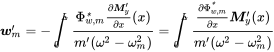
yields the response shape

  (5.12)

The modal coordinates ${\mathit{u}}_n^{\prime }$ are derived by entering this into (5.11) and using the orthogonality of the shape functions providing

  (5.13)

Obviously, the modal density is equal to the pipe solution as it depends only on $c_{LB}$ and $L$.

5.2.2 Bending wave in Finite Beams

In beams, bending waves can propagate with elongation to the direction of the main axes. We skip the analytical closed solution for bending wave motion and stay with the modal shape description for the calculation of bending motion response.

5.2.2.1 Modes

We choose bending motion around the $y$-axis with displacement $w$ in the $z$-direction. The boundary conditions are

  (5.41a)

  (5.41b)

When entering these conditions into the global solution (3.107)

this leads to ${\mathit{w}}_1={\mathit{w}}_2$ and ${\mathit{w}}_{1D}={\mathit{w}}_{2D}=0$. Thus, the mode shape function is

  (5.15)

with $k_n=n\pi /L$. There are also free modes; the solution is a combination of cosine and hyperbolic cosine functions, however, because coefficients ${\mathit{w}}_{1D}$ and ${\mathit{w}}_{2D}$ are not vanishing in that case. The modal wavenumber is similar to the known one-dimensional formulas, but there is a difference for the modal frequency

  (5.16)

The distance between each modal frequency is not constant. So, it is convenient to use the constant wavenumber count of modes that are below $k$

  (5.17)

With this equation we can derive the modal density by applying the chain rule

  (5.18)

This is the same formula as (4.41) but with the group velocity.

5.2.2.2 Modal Response

The displacement in the $z$-direction in modal coordinates is given by

  (5.19)

Entering this into the inhomogeneous form of (3.104a)

  (5.20)

gives for the force distribution

  (5.21)

Multiplication from the right with ${\mathrm{\Phi }}_{w,m}^{*}$ and integration along the beam gives

  (5.22)

A point force ${\mathit{F}}_z$ located at $x_0$ is represented by

  (5.23)

and thus

  (5.24)

From (3.110) we know that ${\mathit{F}}_z=-\frac{\mathrm{\partial }{\mathit{M}}_y}{\mathrm{\partial }x}$, so we can deal with moment excitation using the same modal base

  (5.25)

using the law of partial integration. With the moment ${\mathit{M}}_y$ at $x_0$ described as

  (5.26)

we get

  (5.27)

As moments are linked to the rotations, the derivative of the mode shapes is used.

In Figure 5.2 the response of a beam excited at specific modal frequencies (top) and for a high frequency at different positions is shown.

The spectrum of the point impedance in Figure 5.3 approaches the value for infinite beams (3.136), but has many more peaks than the tube example for high frequencies. This results from the dispersion and the speed of sound that increases with frequency and therefore has fewer modes than rods or tubes.

5.3 Two-dimensional Systems

We deal with plates as an example for a realistic and representative two-dimensional system. In section 3.7 the equation of motion was given for in-plane displacement (longitudinal and transversal) and out-of-plane displacement (bending). The in-plane displacement is characterized by dispersion-free and high-speed wave propagation. Thus, the practical relevance of such systems is not very high as wavelengths stay large in the audible frequency range. For example, a steel plate has longitudinal wave speed of $c_{LP}=4600$ m/s, meaning that we have a wavelength of $\lambda =4.6$ m at 1000 Hz. We would need very large systems to catch the first resonance of this wave type in the audible frequency range and in technical systems as for example a car. Thus, we stay with bending waves for the investigations on two-dimensional systems.

5.3.1 Bending Waves in Flat Plates

For the description of plate waves of finite systems we have to solve the homogenous form of (3.206)

with the following boundary conditions:

  (5.28a)

  (5.28b)

  (5.28c)

  (5.28d)

One can show using the same procedures as Sec. 5.2.2.1 that the function

  (5.29)

is a solution of Equation (3.206) with the modal frequencies

  (5.30)

and

  (5.31)

where $n$ is a double index $n=(n_x,n_y)$. These mode shapes are orthogonal and should be normalized for the product below the surface integral

  (5.32)

leading to the normalised shape functions

  (5.33)

Some shapes are shown in Figure 5.6. The mode count is estimated by the area method but in the wavenumber domain due to dispersion as shown in Figure 5.5. Without tangential modes there are no additional correction areas required.

5.3.1.1 Modal Density

We estimate the number of modes that occur below the wavenumber $k$ by comparing the areas of the quarter wavenumber circle $\pi k^2/4$ to the area covered by one wavenumber rectangle ${\pi }^2/(L_x{L}_y)$

  (5.34)

The modal density of the dispersive bending waves depends on the group velocity {modal density ! plate}

  (5.35)

The dispersion of bending waves leads to the surprising effect that the modal density is constant over frequency.

5.3.1.2 Modal Response

The response of an excited plate can be given by the double sum running over both modal indexes $n=(n_x,n_y)$.

  (5.36)

Entering this into (3.206) we get the modal expression

  (5.37)

and multiplication with mode shapes ${\mathrm{\Phi }}_m^{*}$ and surface integration over the plate gives

  (5.38)

With modal forces

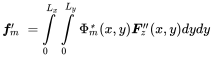  (5.39)

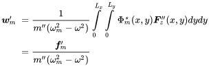
A point force at $(x_0,y_0)$ is represented by a double delta function to create the required force per area function

  (5.40)

leading to

  (5.41)

The mechanical point impedance is

  (5.42)

In Figure 5.7 an example for a point impedance is shown. The boundary impact can also be be neglected here for high frequencies and the impedance value for infinite values is reached. In the case of plates the shape of the impedance curve contains fewer peaks than the beam example. The higher dimensionality of the system provides more “space” for modes. Thus, the dynamic complexity of the system is reached earlier.

5.4 Reciprocity

Similar to the argument in Chapter 4, the reciprocity relationship also holds for structural equations. Inspecting (5.41) it becomes obvious that the quantities force at position 1 (and into direction 1) and the velocity at position 2 (and into direction 2) can be exchanged. Thus, reciprocity in structural dynamics reads as

  (5.43)

The same relationship can be found for displacement and acceleration, even though these quantities are not conjugate. But, they are power related, and a $j\omega$ argument in Equation (5.41) does not change the above arguments. When proving the global principle, it can also be shown that this is also true for coupled systems. Thus, a volume source at position 1 generating a velocity at position 2 is equal to the force excitation at position 2 and the pressure response at position 1. This is of high practical use when the pressure signal of multiple force excitations at the engine mounts of a car are needed. A volume source with accelerometers at all mount positions replaces the experiment with one microphone at the head position and force excitation at every mount position. In complex geometries it may be hard to precisely excite the forces at positions that are not accessible. Placing accelerometers there is usually much easier.

5.5 Numerical Solutions

Due to the fact that we started with mechanical systems of point masses, dampers, and springs, the formulation of the physical interpretation of the mass and stiffness matrices of structural finite elements is clear. In section 5.1 of this chapter, the global dynamic equation in discrete form was formulated. However, even without a deeper understanding, some global properties of finite element models should be given in order to understand the properties and the limits of finite element formulation.

5.5.1 Normal Modes in Discrete Form

In the previous sections of this chapter we learned that modal condensation is a useful tool to calculate the response of mechanical system. The modal method is intensively used in numerical or finite element methods, too. For investigations in later chapters, we will use a discrete variant of the analytical mode shapes from Equation (5.33). The discrete degrees of freedom are $\left\{\begin{array}{c}{\mathit{q}}_i\end{array}\right\}$ defined as shown in Figure 5.9 using a regular mesh. The node with index $i$ is located in the $xy-$plane with nodal position ${\mathbf{r}}_i={\left\{\begin{array}{c}{x}_i,y_i\end{array}\right\}}^T$ and the degree of freedom is the displacement in $z$, hence ${\mathit{q}}_i=\mathit{w}(x_i,y_i)$

Thus, the modal vectors are defined by the nodal position and Equation (5.33)

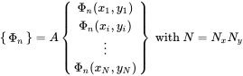  (5.44)

In order to ascertain mass normalization, the mass matrix is required. We assume that the mass of the discretized plate is given by the related lumped mass and thus derived from the specific mass $m^{″}$ times the element surface element that belongs to the specific node. So, we get a diagonal matrix with mass entries $m_i=\mathrm{\Delta }S{m}^{″}$ for inner elements, $m_e=\mathrm{\Delta }S{m}^{″}/2$ for the edges, and $m_v=\mathrm{\Delta }S{m}^{″}/4$ for the vertex nodes.

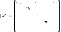  (5.45)

With this assumption the factor $A=\sqrt{\frac{L_x{L}_y}{M}}$ with $M$ as total mass of the plate provides mass normalised modeshapes that can be used for modal frequency analysis or modal condensation

  (5.46)

Due to the fact that the analytical solution is only sampled and the mesh doesn’t have to be fine enough to allow a precise numerical solution, quite coarse meshes can be used, e.g. four elements per wavelength. For a finite element model of the same plate, at least six (linear) elements or nodes per wavelength would be necessary for precise results Bathe (1982).

Bibliography

1. Klaus-Jürgen Bathe. Finite Element Procedures in Engineering Analysis. Prentice-Hall Civil Engineering and Engineering Mechanics Series. Prentice-Hall, Englewood Cliffs, N.J, 1982.