
Appendix A
Basic Mathematics
A.1 Fourier Analysis
We will start our introduction to the Fourier analysis with the series representation of periodic signals. The next step is moving towards the Fourier transform by the application of a limit process. We start with the analytical formulation of the theory: i.e. all signals are continuous, and we will later switch to digital signals in section A.2.
A.1.1 Fourier Series
Imagine a function
This function shall be synthesized by a series of sine and cosine functions, reading
If (A.2) is integrated over the time interval
The first coefficient
Obviously the mean is zero
In Figure A.1 the function and several Fourier series with an increasing number of coefficients are shown. We see that the function is better and better represented, but due to the infinite slope of the rectangular function, an infinite number of Fourier coefficients would be required for a perfect match.

Figure A.1 Rectangular function and its Fourier series representation using up to four non-zero coefficients. Source: Alexander Peiffer.
An entirely equivalent representation can also be formulated by a series of complex Euler functions, this time running from
The coefficients
It is quite illustrative to link these expressions to a harmonic signal with angular frequency
Thus, for a given frequency
An alternative and instructive derivation of this equation can be found by applying an integration over the period for (A.8) multiplied by
If we integrate (A.12) over the period
We see that the right hand side is only non-zero for
This shows in an instructive way how the orthogonality relation is used to derive an alternative expression for
If we replace
With (A.8) we get
Performing the integration and using the orthogonality relationship giving zero for
A.1.2 Fourier Transformation
For stationary periodic processes the Fourier series is the perfect tool to investigate the harmonic content of a signal. The frequency resolution – the difference between two frequencies – is restricted by
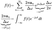
In practical applications many nonperiodic or transient signals occur. For the frequency analysis of such signals we require a finer resolution and a different approach. This can be achieved if we perform the limit process for
Now we let
 (A.20)
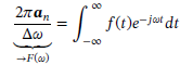 (A.21)
where we have also used
Obviously, the Fourier transform (FT) of a harmonic signal does not converge because the infinite integration requires
with the following Fourier transform
A.1.3 Dirac Delta Function
Based on this rectangular pulse the


Figure A.2 Rectangular pulse function and its Fourier transform. Source: Alexander Peiffer.
The delta function is not a function in the classical sense, because is has infinite values
If the delta function is centred at
The use of the delta function is given by its so-called sifting property that extracts any function if it occurs in the integral over a product with the delta function, such as
The first term of the above equation is called the convolution of
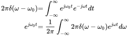
Thus, the frequency content of the delta function extends from negative to positive infinity with a constant value. On the other hand the inverse Fourier transform of the exponential function gives
Exchanging
 (A.32)
A.1.4 Signal Power
The signal power in the time domain is related to the FT similar to (A.18). With
and change of the integration order we get
Using (A.30) enables us to replace the parentheses by
This is known as Parseval’s formula. The total energy in the signal is associated with the integral over all frequency components. If we switch back to the frequency
A.1.5 Fourier Transform of Real Harmonic Signals
Even if the FT of harmonic signals will not provide a finite result, the delta function enables us to apply the FT even to harmonic signals. The cosine function is linked to the exponential function by
Using (A.32) we get for the FT of the cosine function
Applying the infinite integration interval of the FT to the cosine function leads consequently to infinity spectra in the frequency domain, here given by two symmetric delta functions with peaks at
A.1.6 Useful Properties of the Fourier Transform
Working with Fourier transforms is much easier when specific relationships are used that link the time domain with the frequency domain. We start with the partial derivative with regard to time.
Thus, the derivative in time domain corresponds to the multiplication by a factor of
Time reversal in the time domain means complex conjugate in frequency domain.
A further important theorem is the shift theorem which states
This can be easily proven by exchanging variables. A time delay
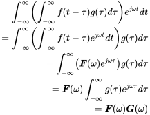
A very important relationship results from the FT of the convolution of two time signals. This is the infinite integral over the product with time delay
The Fourier transform of the convolution gives:
 (A.44)
or
Thus, the Fourier transform of the convolution of two signals is the product of the Fourier transform of each function. It can be further shown that the inverse Fourier transform of a product of spectra is also a convolution in frequency domain.
A.1.7 Fourier Transformation in Space
The Fourier presentation of time signals can be converted to the wave forms in space. We apply the pair of Fourier transformations from (A.22a) and (A.22b) to the space domain
This can be further extended to multidimensional applications, for example two dimensional surfaces
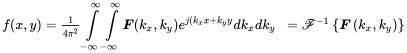 (A.48a)
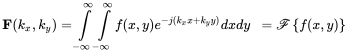 (A.48b)
A.2 Discrete Signal Analysis
Today, most acquisition systems and consumer electronics are based on digital systems. The digital representation of analog or continuous signals is advantageous, because the information can be easily stored and transmitted without losses. This is not the case for analog systems such as, for example, the transmission of frequency modulated radio signals. In addition the results of numerical simulation are also digital. However, the digital analysis and especially the spectral analysis of discrete signals leads to specific effects that must be carefully considered if you would like to avoid mistakes or misinterpretations. The most popular and well known effect is the under-sampling of high frequency data that creates artefacts, e.g. wheels in movies that rotate in the wrong direction. The impact of digital signal analysis is separated into two steps:
- What is the impact of sampling?
- What is the impact of limited signal length or limited number of samples?
We will not consider the discretization effect of sampling. Analog to digital (AD) converters cannot present the samples in a continuous way. However, due to the vast development of AD converters and digital systems, 24 bit is used even for consumer electronics. This corresponds to a dynamics larger than 16 million or 140 dB, which is often higher than the signal to noise ratio of the sensor–amplifier system.
A.2.1 Fourier Transform of Discrete Signals
For dealing with this phenomena, a mathematical formulation of the sampling process is required. The sampling can be represented by multiplying the continuous signal by a sum of delta functions
called a delta comb. Here,
and get with the sifting property
In Figure A.3 the results of Equation (A.49) are presented graphically. The continuous function is now represented by an infinite train of delta functions. The area of each delta peak at
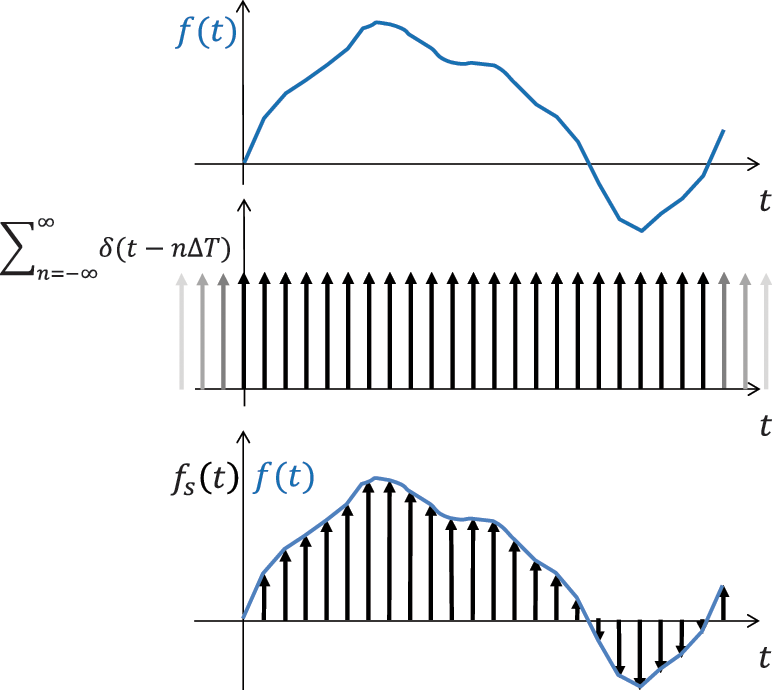
Figure A.3 Process of sampling by a delta comb function. Source: Alexander Peiffer.
The sampling has a very peculiar effect on the Fourier transform. Note that the discrete FT has an argument of the form
In the Equation (A.15) for the complex Fourier coefficients
With these coefficients the Fourier series of the delta comb is given by
Entering this into (A.50)
as far as rearranging sum and integration of the Fourier spectrum of the sampled signal leads to the following expression
This term in parentheses is the Fourier transform with frequency argument
Thus, the sampling of the function

Figure A.4 The Fourier transform of the sampled signal with its periodically repeated continuous spectrum at intervals of
In Figure A.5 the spectrum of the sampled signal is shown when the analog signal has frequency contributions above the maximum frequency

Figure A.5 The Fourier transform of a sampled signal with overlapping spectra due to spectral content above the maximum sampling frequency. Source: Alexander Peiffer.
We can conclude on the first question: What is the effect of sampling? The sampling process gives a discrete set of data values approximating the continuous signal. The frequency domain of the original spectrum is converted into a periodic spectrum with frequency interval
A.2.2 The Discrete Fourier Transform
As digital signals will not contain an unlimited number of samples, the infinite sum has to be replaced by a sum over
From this formula all continuous values of
and the discrete Fourier transform reads
It can be proven (see e.g. Oppenheim et al., 1999) that we can exactly recover the samples
To conclude, the finite number of samples (and not the sampling procedure) causes a finite number of samples in the Discrete Fourier transform. In numerical tools the above formulas of the DFT are implemented in a numerically more efficient way: the Fast Fourier transform (FFT). A special algorithm is implemented that recursively calculates the DFT but only for
A.2.3 Windowing
In principle we have all the means to investigate time signals and their spectral content numerically. There is one remaining issue that is worth mentioning. The spectrum is sampled at discrete values. What happens when we analyze a harmonic signal of frequency
In order to illustrate this, we switch back to continuous signals. The finite number of samples of the DFT can be interpreted as a rectangular window function. So we multiply the time signal with a function
According to (A.46) this results in a convolution in frequency domain
In other words, the spectrum of a windowed function is the convolution of the FT with the FT of the window function. The FT of a rectangular window that is defined as follows
has the FT in the form of a sinc function
Consider now the spectrum of a cosine function (A.38) that consists of two symmetric peaks. When convoluted with the FT of a window function, the spectrum looks as shown in Figure A.6 where the FT of the window appears at the positions of the delta function. The peak of the window function is given by
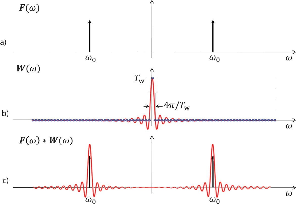
Figure A.6 Effect of windowing on the spectrum of the cosine function. Source: Alexander Peiffer.
being
In Figure A.6b the shape of the windows FT is shown, and the sampling of the related discrete FT is denoted by blue dots. The sampling occurs exactly at the zeros of the sinc function. Thus, when the frequencies of the cosine function fit exactly to one spectral sampling value, you get a single peak. What happens if this is not the case? In this case the sampling occurs at the sides of the window peak that is very steep so that the amplitude is underestimated. This is called spectral leakage.
For avoiding this there are two options:
- We increase the spectral sampling rate by extending the time interval artificially by adding zero values to the time signals, the so-called zero-padding.
- We use a window function with a broader peak in the frequency domain to mitigate the leakage effect.
An often used window function is the Hanning window given by
The effect of this broader window is sketched in Figure A.7. The leakage is reduced, but a certain underestimation of the amplitude is still possible.

Figure A.7 Cosine function spectrum with Hanning windowing function. Source: Alexander Peiffer.
Mitigating spectral leakage requires compromises; either you need fine spectral resolution, but then you accept high leakage. When choosing a broad peak you reduce the leakage but you loose spectral resolution. A further option is to take a higher number of samples or increase the time length
The sample interval in the spectrum is
A.3 Coordinate Transformation of Discrete Equation of Motion
The conversion between coordinate systems is a useful means to reduce the size of the numerical problem, for example to change from global coordinates to local dynamic coordinates with an easier formulation of the dynamics.
The equation of motion in discrete form
shall be converted into the coordinates
Here,
and multiplying from the left with
So, the matrix and force are converted into the new system by
Note that from Equation (A.69), the matrix must be invertible and therefore consist of linear independent vectors.
Bibliography
- M. Frigo and S. G. Johnson The Design and Implementation of FFTW3. Proceedings of the IEEE, 93(2): 216–231, 2005. ISSN 0018-9219.
- Alan V. Oppenheim, Ronald W. Schafer, and John R. Buck. Discrete-Time Signal Processing. Prentice Hall Signal Processing Series. Prentice-Hall, Upper Saddle River, NJ, second edition, internat. 1999. ISBN 978-0-13-083443-0.
Notes
- 1 This is not the length of the delta peak, because this is infinite