
9
Deterministic Applications
In technical acoustics deterministic systems are usually treated by numeric methods like the finite element method or the boundary element method. Those methods require complex and powerful solvers as far as pre and post-processors to handle large and detailed models. Even though such models are extremely useful for the simulation of vibroacoustic systems, it is hard to develop a deep understanding of the dynamic phenomena with these numeric models and to draw the right conclusions.
In this book we will treat deterministic systems as far as possible by analytical approaches or by models that consist of sub-elements that can be described by analytical formulas. This allows the reader to follow and understand the details of the theory and may help to provide a deeper understanding of typical vibroacoustic systems. However, even with such constraints, the examples in this chapter are about several deterministic subsystems that are used in real technical systems and create the basement for later SEA or hybrid FEM/SEA examples.
9.1 Acoustic One-Dimensional Elements
One-dimensional acoustic elements are used in the simulation of mufflers, ventilation systems, or hydraulics. The wavelength is assumed to be much larger than the dimension of the cross section. Such systems can become very complex, and they are also used as a designed network in audio systems, for example, the housing and resonators of loudspeakers. In the context of this book, these elements are presented as typical deterministic applications in order to explain the different effects of filters, resonators, and absorbers.
9.1.1 Transfer Matrix and Finite Element Convention
When dealing with one-dimensional systems, the literature often refers to the transfer matrix theory (Pierce, 1991; Mechel, 2002). This approach is useful when the full system is also one-dimensional, meaning that it is a linear chain of subsystems without additional branches.
In Figure 9.1 the convention for both is shown. When the pressure (or the velocity) is used as state variable the mobility matrix reads as (4.11)

Figure 9.1 Convention for stiffness matrix and TMM. Source: Alexander Peiffer.
or the impedance matrix
The velocity in equation (9.2) is a shared internal degree of freedom, and the pressure corresponds to an external pressure as discussed in Xue (2003). Thus, due to the continuity of pressure (or force), we assume for the external pressure on the right hand side.
In the transfer matrix method theory the situation is different – here the pressure is the internal pressure or the state variable, and .
To conclude, when we switch from the transfer matrix method presentation to FE, the right hand side internal pressure is the negative internal pressure: . In the following we will use in the mobility presentation and in the transfer matrix approach. The transfer matrix representation of the same system is:
Both representations can be easily exchanged. Solving the above equation for each different state variable gives
When the system consists of a cascade of one-dimensional systems, the transfer matrix method is very convenient
because the total transfer matrix is the product of all transfer matrices
This makes the calculation fast and simple, because no matrix inversion is involved. However, the FE approach is more straightforward and allows for branches in the total system.
9.1.2 Acoustic One-Dimensional Networks
Acoustic networks consist of systems with specific cross sections at both ends. Thus, it is useful in accordance with the finite element formulation from section 4.3.2 to switch from velocity to volume flow. This is the continuous quantity at connections as shown in Figure 9.2
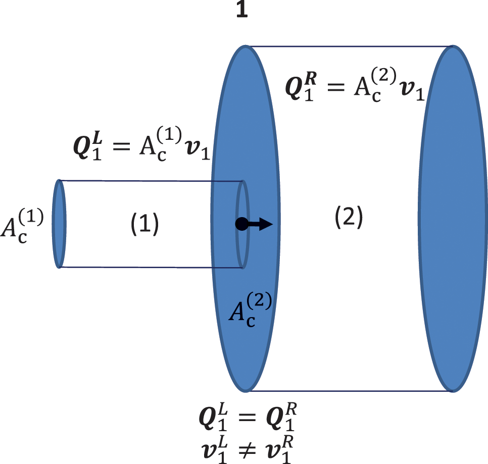
Figure 9.2 Connection of one-dimensional acoustic systems of different cross sections. Source: Alexander Peiffer.
The appropriate matrix equation to describe this would be the radiation mobility matrix with the pressure as internal state variable and the volume flow as external excitation quantity.
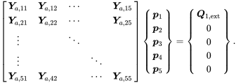
An example for an acoustic network is shown in Figure 9.2. Here the net flow into the nodes is zero when no external volume source is applied. In the final matrix equation, the state variables are calculated and must be derived from the impedance of the connected and cut-free subsystems. So, the flow into each node determines the nodal pressure as state solution. We use the following convention: The flow denotes the volume flow into the node from the system .
The equation of motion for the acoustic system as shown in Figure 9.3 is
 (9.9)
(9.9)
Figure 9.3 Acoustic network with nodal volume flow, volume sources, and radiation impedance at open ends. The numbers in circles denote the system numbers. Source: Alexander Peiffer.
Equation (9.9) is derived by using the element mobility from (9.8) and adding each element mobility to the total system matrix similar to the procedure described in section 4.3.1 but with a different source term.
This finite element formulation is efficient when used as a numerical solution but not when analytical expressions are required. The network equation must be solved or inverted to get the system response. Inverting the analytical formulas is not easily done or possible in many cases, and the transfer matrices are more useful.
According to the discussions regarding the transfer matrices in section 9.1.1, we can change easily between the different formulations. The transfer matrix reads as:
and the conversion between each representation is
Thus, for one-dimensional acoustic networks with changing cross section, equation (9.10) may be the best choice.
9.1.2.1 Properties of the System Matrices
From the reciprocity principle some useful properties can be derived. Reciprocity states
Entering this into the two port equation gives for this mobility matrix
Hence, they are symmetric. The transfer matrix is obviously not symmetric which can be seen from equations (9.5) and (9.12). From the same equations it can be derived that the determinant of the transfer matrix equals 1
9.1.3 The Acoustic Pipe

Figure 9.4 Properties of an acoustic pipe. Source: Alexander Peiffer.
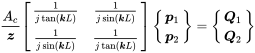
We take the acoustic pipe from section 4.1 and switch to the volume flow using ; we get the radiation mobility matrix formulation with pressure as state variable and the volume flow as external source from equation (4.11):
 (9.16)
The transfer matrix representation reads as:
 (9.17)
9.1.4 Volumes and Closed Pipes

Figure 9.5 Closed volume and pipe. Source: Alexander Peiffer.
The closed volume was derived in section 4.3.1 leading to equation (4.98). We divide this equation by in order to get the mobility version with as source term
The bulk modulus can be replaced using (2.18), giving
The volume formulation assumes a volume extension to be much smaller than the wavelength. For thin cylinder shaped volumes, the one-dimensional pipe formulation with rigid end (4.16) leads to
This equation is more appropriate for volumes that have only cross section dimensions that are small compared to the wavelength but can have large dimensions in the direction of sound propagation. However, when , the tangent can be approximated by , and equation (9.20) leads to
This is exactly corresponding to expression (9.19). We conclude with the mobility of the volume and tube, namely
and the according impedances from the reciprocal.
9.1.5 Limp Layer
This generic model describes a lumped element in the pipe flow, representing mass, stiffness, or damping effects. The condition for the validity of lumped elements is that the wavenumber must be much larger than the dimension of the element. Thus, we assume .
As shown in Figure 9.6, the lumped element presentation has in common that the volume flow or velocity is equal on both sides. Thus, the dynamic behavior can be described by transfer impedances

Figure 9.6 Mass and stiffness element in a pipe of cross setion . Source: Alexander Peiffer.
The transfer impedance can be written in the following way:
The real and imaginary parts represent the reactive and dissipative parts, respectively. The transfer matrix of such an element is then determined by reshuffling the above equations to an appropriate set
and the transfer matrix of the generic layer reads as:
According to the transformation in (9.11) the radiation mobility matrix representation is
In the literature the transfer matrix is often used to describe the acoustics of specific layers.
9.1.5.1 Mass
Mass layers can be limp membranes that are closing the pipe or plates that are in the pipe where friction can be neglected. For example, a thin fluid layer of small thickness can also be approximated by a mass layer. Following Newton’s law , the equation of motion is
Similar to the discussion concerning volume and pipe end the mobility expressions can also be derived as an approximation of equation (9.16) for small values of .
9.1.5.2 Stiffness
A stiffness in the pipe can be thought of as an infinitely stiff plate supported by a spring of stiffness or a specific stiffness . The equation of motion for a spring leads to

Figure 9.7 Cylindrical membrane exposed to pressure. Source: Alexander Peiffer.
9.1.5.3 Viscous Damping
The viscous damping is determined by , and hence
We see that the damping results in the real resistance , whereas the imaginary part considers mass and stiffness effects . The total transfer impedance is hence
9.1.6 Membranes
A practical implementation of a system with mainly mass and stiffness is a membrane with tension mounted in a circular cross section . From the membrane equation of motion (3.139)
and using the cylindrical Laplace operator we get
When we assume a circular membrane with boundary condition , the solution is
When we derive the limp parameter, we have to use the surface averaged quantities. The stiffness can be defined based on the volume change due to the static pressure:
The area specific stiffness is defined by and the volume is given by
Thus, the stiffness of the membrane is
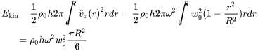
The membrane is displaced non-uniformly. For the efficient mass estimation we use the displacement and calculate the kinetic energy based on this
The velocity maximum occurs at zero displacement position
This energy must be equal to the kinetic energy of the membrane movement integrated over the given velocity shape
 (9.40)
Setting both kinetic energies equal leads to the efficient mass
or the specific mass
which corresponds to of a mass layer. Thus, the final reactance of the membrane is:
9.1.7 Perforated Sheets
Perforated sheets are a major device for acoustic treatment in engineering acoustics. Consider for example the ceiling of typical offices showing perforated surfaces or surfaces with a regular grid of holes. Such systems provide control over the parameters mass, stiffness, and damping. As a first attempt one might consider the volume in the hole as a mass with plus a specific end correction resulting from a fluid volume partition that is moving on both ends of the channel. But, the channels are supposed to be so small that the wave motion is affected by friction at the walls, and we have a certain flow profile in the hole. A detailed treatment of this theory would go too far, but an established model is derived by Maa (1998) and extended with further details by Fuchs and Zha (1995).
In order to get more insight, only the basic concepts of Maa’s model are given here. The pore is assumed to be cylindrical and so small that friction is affecting the flow profile in the fluid. Maa derived that the velocity profile is given by
with
and as shear or dynamic viscosity. In order to get the average or efficient velocity we have to integrate over the cross section
When we assume small hole depth compared to the wave length we can assume and thus:
So, we found the right expression for a single hole. The holes are covering only part of the surface. Thus, when averaging the velocity over the surface we have to consider this. The ratio of hole surface to total surface is the surface porosity , and the efficient velocity related to the total surface S is
and finally we get
The surface porosity can be derived from the distance of the hole in a square grid as shown in Figure 9.8.

Figure 9.8 Geometry of a perforated plate with square grid. Source: Alexander Peiffer.
In principle we have found the transfer impedance that is required to describe the dynamics of a perforated layer. But, there are some modifications required:
- The flow outside in the nearfield of the pore must be considered.
- The Bessel functions are quite unwieldy and should be simplified.
The first item is addressed by the so called end corrections. They consider the mass of the fluid above and below the pores and the additional friction at the pore edges. The second item is address by an approximation of the Bessel functions that leads to a maximal error of 5% (Fuchs and Zha, 1995).
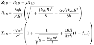
Finally, the approximation derived by Maa and extended by the nearfield corrections in FreeFieldTechnologies (2015) is:1
 (9.50)
with being a constant that is considered to be for sharp edged holes and for round edges; depends on the porosity and the grid pattern and is given by
For a squared grid .
9.1.7.1 Example for a Micro Perforated Grid
The task of perforate is to provide specific acoustic mass and flow resistivity for absorber applications. In Figure 9.9 the normalized transfer impedance of a perforate with thickness mm, hole radius mm and squared grid distance mm is shown. The porosity is .

Figure 9.9 Normalized transfer impedance of perforate mm, mm, mm and . Source: Alexander Peiffer.
The normalized resistance is near 1 thus equal to the impedance of air. This means the perforate is well adapted to plane waves in air. The reactance shows an increase in mass by the nonlinear slope or the reactance curve resulting from viscosity effects in the pores.
9.1.8 Branch Lumped Elements
Additional to the transfer impedance, we define a branch element with radiation impedance . The situation is contrary to the transfer impedance. As shown in Figure 9.10, the pressure is constant at both ports, but the volume flow is not.

Figure 9.10 Branch impedance configuration of the pipe network. Source: Alexander Peiffer.
This leads to the transfer matrix presentation:
Any expression for this branch equation can be used – for example, the piston radiation impedance or the results from section 9.1.5.
9.1.9 Boundary Conditions
The boundary conditions in the network descriptions are required to define end conditions by the ratio of pressure and velocity. For the volume flow as state variable, an open end corresponds to zero pressure. When pipe systems are given, they may be excited by sources with an inner impedance, and one end might radiate into the free field. Thus, for realistic systems an impedance end condition must be defined. This could be the characteristic impedance of one-dimensional wave propagation or the radiation impedance of a piston (9.95).
The single node expression for the impedance in the finite element expression is
When we assume the free field boundary condition, the mobility values are
or in case of the pipe ending in a semi infinite space, the radiating piston would be more appropriate; in this case must be replaced by the impedance from equation (9.95). For unbaffled configurations the radiating sphere would be more realistic, using equation (2.84) for .
In case of the transfer impedance description, we set one value of the state to 1, say the velocity. In the cascade transfer matrices, the inputs of the first state vector are
9.1.10 Performance Indicators
Evaluating such networks aims at a certain effect on the noise propagation. So, we need parameters that describe the effect or performance of such networks. In general the above described systems can be set up and solved for any source and receiver configuration. There are two kinds of indicators: one is a comparative criteria given by the pressure or transmitted power with and without the device, and the other parameter is a local absorption criteria.
9.1.10.1 Transfer and Insertion Coefficients
The performance indicator results from the comparison of a reference system to the newly designed system. The ratio of squared result variables is called the insertion loss as defined in equation (2.169)
A further quantity for system performance is the transmission coefficient.
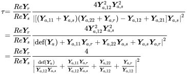
In Chapter 8 the transmission coefficient definition results from diffuse field reciprocity and the coupling of semi infinite systems. Equations (8.8a) and (7.27) can be used to calculate the transmission factor for a one-dimensional system by adjusting the mobility of impedance degrees of freedom to the stiffness coordinates. In the literature there are several derivations using the transfer matrix approach, for example Allard and Atalla (2009), Tageman (2013), or Jacobsen (2011). Here, the mobility matrix approach will be used.
As can be seen in Figure 9.11, an arbitrary system is extended by the radiation mobilities and for sender and receiver, respectively. The input power is given by

Figure 9.11 Reference and test system configuration for the definition of the transmission. Source: Alexander Peiffer.
because the pressure and the (internal) volume flow are given by the entry boundary condition. The reference system is described by two connected equal mobilities , so an external source leads to the pressure
and finally:
The power radiated to the receiver mobility is:
In a complex network with many nodes, the network matrix equation (9.9) must be solved to calculate the output pressure of the network and the radiation mobilities. In order to cope with an input and output description, the network matrix must be condensed to the external degrees of freedom. Thus, the assumption of a 2x2 matrix is not a constraint of generality, and the result can be compared to the transfer matrix theory. A general one-dimensional system as shown in Figure 9.11 with radiation impedance endings is described by:
Matrix inversion gets from , and we consider that there is no source at port 2 hence :
So, the pressure is given by
Entering this into (9.62) gives
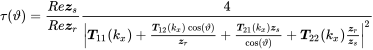
This reads for the transmission factor
When we have condensed the network, this expression defines the transmission through the network. We rearrange the details of the total matrix determinant
 (9.68)
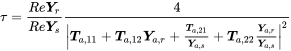
and convert this into the transmission values using equation (9.12)
 (9.69)
corresponding to expressions in the literature. When both media are the same, , then
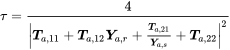 (9.70)
9.1.10.2 Absorption
The absorption is also derived in Chapter 2, namely by equation (2.105) for . The relevant quantity in this context is the input impedance. In the network context we have to solve the FE equation for loads at the input, say . The input impedance follows from the resulting pressure
leading to the selected absorption depending on the impedance of the connected system.
9.2 Coupled One-Dimensional Systems
In Section 9.1 the finite element representation of typical systems was developed to simulate acoustic networks. In the following we will elaborate some examples created by such subsystems.
9.2.1 Change in Cross Section
The changes in cross section motivated the selection of the volume flow as state variable. As a consequence the cross section element is supposed to be very simple, and the transfer matrix is the unit matrix
Assuming the same fluid on both sides, the transfer coefficient reads, with and :
 (9.74)
9.2.2 Impedance Tube
The impedance tube is a device to measure the surface impedance of a specimen, for example a layer of foam, an absorber, or natural wall surfaces. In Figure 9.12 the impedance tube set-up is shown.

Figure 9.12 Impedance tube for measuring the surface impedance of a flat probe. Source: Alexander Peiffer.
We search for the dependency of the two measured pressures at positions and from the contact impedance at the end. In principle equation (4.15) can be applied directly, but in order to present the use of the transfer matrix method, we use it here.
The transfer matrices between and as far as and are given by
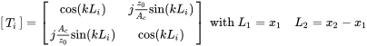 (9.75)
The end condition is given by (9.57) with . The pressure follows from
and from
Using the pressure ratio and solving for gives:
9.2.3 Helmholtz Resonator
The Helmholtz resonator is the acoustic network representation of a tuned vibration absorber. Spring, mass, and damper are realised as fluid devices. The construction is as shown in Figure 9.13 on the left hand side.

Figure 9.13 Helmholtz (LHS) or quarter wave resonator (RHS). Source: Alexander Peiffer.
This cascade of involved subsystems can be readily described by transfer matrices. The neck of length works as a mass of and thus with transfer impedance and resulting in the transfer matrix
For the neck we follow the same argumentation as for the pores in the perforate absorber. We may have different situations as shown in figure 9.14. When there is no perforate at the opening, the resonator may use an end correction representing a fluid cylinder of length on both sides if the jump in cross section is very high, thus . As shown for the low frequency approximation for the piston in the wall (2.156), this length is with being the radius.

Figure 9.14 Neck tube with different end corrections. Source: Alexander Peiffer.
If the opening is covered by a perforate, this end correction can be replaced by the transfer impedance of the perforate. The correction length at the connection of the volume is taken into account by the length correction adjusting . The end correction at the opening is included in the general transfer impedance term.
The end condition at the degree of freedom 2 is given by the volume form equation (9.22) and (9.57):
The classical Helmholtz resonator is open, but in some applications the neck is covered by a perforate. In order to keep the option free, we represent the perforate by the generic transfer impedance
In case of an open neck, the reactance is determined by the end correction as discussed before:
When covered by a perforate, the transfer impedance is given by equation (9.50) converted into a radiation impedance
The total transfer matrix follows from
and the surface impedance is given by
Thus,
The system is in resonance when the imaginary part is zero, and for the pure resonator without porous sheet we get
At resonance the input impedance is . Thus, for specific frequencies the Helmholtz resonator creates a matching end that would not be possible at low frequencies with such small dimensions. In Figure 9.15 the radiation impedance of one example resonator is shown. At resonance () the reactance curve crosses zero creating a purely resistive impedance at resonance frequency.

Figure 9.15 Radiation impedance of Helmholtz resonator of parameters mm, cm3 and mm. Source: Alexander Peiffer.
When we need a perfectly matched end at a specific frequency, the Helmholtz resonator is the best choice for restricted space. Using the perforate of section 9.1.7.1 at the ending, the resonance moves to higher frequencies. This is because the upper mass is missing, but the resistance matches perfectly . The results are shown in Section 9.2.4 in combination with the quarter wave absorber.
9.2.4 Quarter Wave Resonator
The quarter wave resonator is similar to the Helmholtz resonator except the fact that the resonator does not clearly separate between the mass (neck) and spring (volume) part. It consists of a tube with length with rigid end and the same end correction as for the Helmholtz resonator neck. From section 4.1.1 and equation (4.17), we know the input impedance of the resonator.
The impedance is zero for with so the resonance frequencies are
With the transfer impedance for end correction of perforate consideration
Deriving the input impedance from this we get
We may consider the transfer matrix of both end correction (9.82) and (9.83). Quarter wave resonators are rarely used without cover. They are covered in most cases by perforate, for example in the liner absorber of turbofan engines. The perforate from the last section can be used together with a resonator length of mm.
In Figure 9.16 the impedances of both resonators are shown. The resonance frequency of the Helmholtz resonator is lower as for the quarter wave version. This results in better low frequency absorption as shown in Figure 9.17.

Figure 9.16 Radiation Impedance of Helmholtz resonator of parameters mm, cm3, and mm and quarter wave resonator mm and perforated sheet. Source: Alexander Peiffer.

Figure 9.17 Absorption coefficient of Helmholtz resonatorand quarter wave resonator. Source: Alexander Peiffer.
9.2.5 Muffler System
Mufflers are applied to reduce, for example, the noise of combustion engines or other machinery that creates pulsating volume flow in the audible frequency range. Here, we neglect any flow component by assuming that the flow speed is much lower than the speed of sound. More details for realistic mufflers can be found in Munjal (1987).
9.2.5.1 Expansion Chamber
A simple muffler consists of a combination of three tubes as shown in Figure 9.18. A pipe of cross section is expanded in the middle to a specific cross section ; this leads to 3 tube sections. As this is a cascaded set-up the transfer matrix method can be applied.

Figure 9.18 Expansion chamber arrangement a) reference system b) expansion system. Source: Alexander Peiffer.
The system is described by the matrix product of all sub pipes using equation (9.17) with according length and cross section
or we use the mobility form setting up the system matrix.
9.2.5.2 Open end Conditions
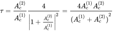
We start with the case that source impedance and end impedance are considered as one-dimensional free field . In this situation the first and third pipe in Figure 9.18b can be neglected, and the total system performance is defined by the expanded chamber in the middle. From equation (9.70) we get
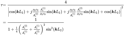 (9.93)
or expressed as transmission loss
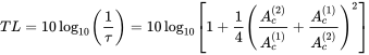 (9.94)
In Figure 9.19 different transmission losses are shown. The higher the change in cross section, the better the performance. We see that for sources in a well defined frequency range, a transmission loss of more than 30 dB can be achieved. However, when the center chamber is in resonance the transmission loss is zero, and the muffler does not work.

Figure 9.19 Transmission loss of expansion chamber with various cross section ratios; cm. Source: Alexander Peiffer.
9.2.5.3 Realistic End Conditions
Every muffler pipe radiates finally into the three-dimensional space. Thus, the pipe end will have the piston radiation impedance. In this case the first and third pipe of the system must be included, because reflections will occur at both ports.
The radiation impedance of the piston, according to equation (2.152), is:
When the matrix is built up as explained in section 9.1.2, we can consider each detail of the setup. We still assume an open condition at the source and compare the muffler to the reference pipe of same total length. The parameters of the expansion chamber are given in Table 9.1; the given center radius corresponds to an area ratio of 10.
Table 9.1 Expansion chamber geometry parameter
| Tube | Length | Radius |
|---|---|---|
| 1 | cm | 5 cm |
| 2 | cm | 15.8 cm |
| 3 | cm | 5 cm |
The pressure magnitude at the end of the reference tube and expansion chamber is shown on figures 9.20 and 9.21. In the reference chamber the piston end condition leads to reflections that are seen at the entry. The expansion chamber shows several resonances coming from the the different pipe sections. Globally the pressure is reduced, but there are still some resonances where the muffler has a weak performance.

Figure 9.20 Pressure at entry (node1) and end (node4) of the reference tube with flanged end. Source: Alexander Peiffer.

Figure 9.21 Pressure magnitude of expansion chamber at entry (node 1) and end (node 4), and at entry (node 2) and end (node 3) of the expansion chamber. Source: Alexander Peiffer.
The performance is qualified by the insertion loss comparing the pressure of reference and muffler system. The result is shown in figure 9.22. We see that at some frequencies, there are negative values, meaning that the reference system is more efficient than the muffler. Thus, real mufflers require additional damping, realized for example by steel wool, to take care of the resonances.

Figure 9.22 Insertion loss of expansion chamber. Source: Alexander Peiffer.
9.2.6 T-Joint
This system makes use of the Helmholtz resonator as a resonant damper in the one-dimensional propagation path. Such devices are called T-joints and are applied in hydraulic pipes to fight pulsation from hydraulic pumps or to reduce noise in the engine air intake. In Figure 9.23 a typical set-up is shown. The Helmholtz resonator is located in the middle, hence cm, the source impedance is open, and the end dynamics is given by the piston radiation impedance. The system can be described both ways: either the FE method using the Helmholtz resonator impedance as boundary condition at the center node, or by applying the transfer matrix method with a branch impedance.

Figure 9.23 Pipe with t-joint and connected Helmholtz resonator. Source: Alexander Peiffer.
In this example we use Helmholtz resonators of the following parameters: , cm3, and cm. We use the pure Helmholtz resonator configuration and with a perforate cover in order to show the effect of damping. The perforate parameters are thickness mm, hole radius mm, and porosity . Such radiation impedance of both resonators is shown in Figure 9.24; we see a relative moderate resistivity of approximately , and the resonance of both is at Hz.

Figure 9.24 Transfer impedance of T-joint perforate mm, mm, and . Source: Alexander Peiffer.
With the pure Helmholtz resonator, the insertion loss can be very high, as can be seen in Figure 9.25, but showing some negative loss at some resonances. The perforate version is not as effective but avoids the negative insertion loss.

Figure 9.25 Insertion loss of T-joint system with and without perforate. Source: Alexander Peiffer.
9.2.7 Conclusions of 1D-Systems
In the last section a set of system and tools was developed to deal with one-dimensional fluid systems, namely pipes or tubes. Besides the practical use of such systems, the idea was to present means of noise control that are based on deterministic and coherent devices. From the point of view of the vibroacoustics engineer, the design and layout means adjusting the different resonances correctly.
9.3 Infinite Layers

Figure 9.26 Wavenumbers in x and z-directions for infinitely extended layers. Source: Alexander Peiffer.
Infinite layers are one-dimensional systems which are infinite in the other two dimensions. The infinity guaranties that plane waves can propagate in all directions, and the projection of the wave propagation normal to the plane is a one-dimensional wave motion. From the space vector definition in section 8.2.3, it is clear that the components of the wavenumber determines the in-plane state, whereas defines the propagation through the layer. For homogeneous layers we set without loss of generality. We take an infinite layer of fluids and a plane wave impinging at angle ; the wavenumber parallel to the surface is . The coordinate in the -direction is given in wavenumber space by . In case of infinite layers – and only then – remains constant in each layer, and only varies. The in-depth wavenumber depends on the speed of sound in the layer. Thus, it is . The transfer matrix method is converted to an infinite layer by adding a wavenumber argument to the transfer matrix.
9.3.1 Plate Layer
The mass layer can be enriched by bending stiffness effects using the results from section 8.2.4.3. Using the Ansatz of plane waves again this reads
For infinite plates the displacement must have the same wavenumber
entering this into the wave equation of the plate (3.206) leads to
and the transfer impedance is
After some modification the transfer impedance reads as:
For zero bending stiffness , the transfer impedance is showing that the limp behavior does not depend on the wavenumber . As there is no in-depth wave propagation, the transfer matrix has the same form as (9.27) with the above given transfer impedance.
9.3.2 Lumped Elements Layers
In general, the parameters of lumped elements don’t change due to the wavenumber argument. So, mass layers and perforates can be used as is. The given transfer impedances according to (9.27) or specifically for the mass layer (9.29) or the perforate (9.50) are still valid.
9.3.3 Fluid Layer
The transfer matrix method of one layer excited by a plane wave of follows from the solutions of the wave equation in the -direction. We slightly modify equation (4.1)
keeping in mind that
is a function of . We get in accordance with the one-dimensional fluid transfer matrix method
 (9.106)
9.3.4 Equivalent Fluid – Fiber Material
Fiber materials are used for acoustic isolation and absorption. The acoustic fluid motion in the fiber network leads to losses in the flow and wave propagation. The deceleration of the fluid motion acts on the fiber matrix and accelerates the fibers. A model for such porous materials is mandatory for noise control application, but the required theory is out of scope for this book. Allard et al. (2005) provides a comprising overview about the acoustic theory and application of porous material.

Figure 9.27 Sketch of fiber absorber. Source: Alexander Peiffer.
We use the model of the limb equivalent fluid that was developed by Champoux for the rigid or fixed matrix Champoux and Stinson (1992) and extended by the limb frame model as described, for example, by Paneton Panneton (2007). The useful thing with this model is that the acoustics in the fiber material are still described by acoustic fluid parameters. They become complex and frequency dependent, but the existing models of fluid layers or tubes can still be used. A thorough description by complex models – as for example Biot models Biot (1962) – considering the two coupled waves in the solid and fluid phase, require a completely different approach handling several degrees of freedom and connectivity conditions. In order to keep the efforts reasonable, we leave it with the simple presentation of the final formulas:
 (9.107d)
There is a confusing variety of parameters that are not all independent as shown by Horoshenkov et al. (2019). A heuristic explanation of the parameters is given in tables 9.2 and 9.3.
Table 9.2 Fiber parameters of the equivalent fluid model
| Symbol | Description |
|---|---|
| Volume porosity, fraction of fiber and total volume | |
| Tortuosity, ratio of average path through the absorber to straight path, | |
| a measure for the diversion of the fluid | |
| Viscous characteristic length | |
| Thermal characteristic length | |
| Static air flow resistivity | |
| Apparent total density of fluid and fiber | |
| Equivalent density of the fluid in a rigid/fixed fiber matrix | |
| Equivalent density of the limp equivalent fluid |
Table 9.3 Fluid parameters
| Symbol | Description |
|---|---|
| Fluid density | |
| Dynamic viscosity | |
| Prandtl number |
Table 9.4 Material parameters of soft fiber material. Source: Panneton (2007).
| Symbol | Value | Units |
|---|---|---|
| 0.98 | ||
| 25 000 | N s/m4 | |
| 1.02 | ||
| 90 | m | |
| 1.208 | kg/m3 | |
| 31.1 | kg/m3 | |
| 1 For fibrous material can be assumed. | ||
The soft fibrous material from Panneton (2007) is taken as an example. In figures 9.29 and 9.28 the results for the complex speed of sound and the density show a strong dependency on frequency. The are two major versions of equivalent fluid models: the rigid frame model, assuming a fixed fiber matrix with no participation of the fibers to the motion, and the limp frame model that considers forced motion of the frame inertia. One can easily switch from the rigid to the limp model by using equation (9.107)c. For low frequencies the real density of the limp model reaches values near the bulk density of the material, because the material moves with the inertia of the bulk material. The rigid frame model does not catch this effect. In the high frequency limit, both models provide the same result. According to Panneton the high frequency limit is

Figure 9.28 Dynamic complex density of limp and rigid fiber material. Source: Alexander Peiffer.

Figure 9.29 Dynamic complex sound speed of limp and rigid fiber material. Source: Alexander Peiffer.
A similar effect can be seen for the speed of sound. For high frequencies the real value of the limp model reaches the real value of the rigid model. At low frequencies the speed of sound of the fiber material is below the fluid sound speed because of the additional density from the bulk material. In Panneton (2007) the results are compared to tests, showing that the rigid frame model fails for low frequencies.
To conclude, for the calculation of fiber material sound propagation, we presented a useful model that is, for example, used frequently in aerospace applications (Moeser et al., 2008).
9.3.5 Performance Indicators
The performance indicators from the last section are reused here but with wavenumber or angle as argument and now formulated for the impedance instead of radiation mobility. The source and receiver impedances of the fluids are also dependant on the angle of attack due to equation (2.116). With we get
 (9.109)
The diffuse field performance is derived by equations (8.13) or (8.14). The above formula is often used with an empirical maximum angle leading to the formula shown in (8.103). When we are interested in the absorption, we have similar modifications for (9.72)
 (9.110)
getting an according diffuse field absorption by angular averaging
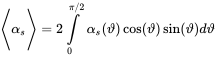 (6.72)
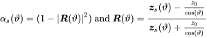
For normal irradiation the perfect absorption is achieved for , thus a perfectly matching impedance with zero reactance and resistance equal to the characteristic impedance of air. However, this condition cannot be met for all angles of incidence. In the diffuse field integration the most important angle is , because the -term in equation (6.70) has its maximum at this angle.
In Figure 9.30 the diffuse field absorption is calculated for different values of the real surface impedance. We see that highest diffuse field absorption can be achieved by with . So, the design goal for a best diffuse field absorbing device is given by this rule.
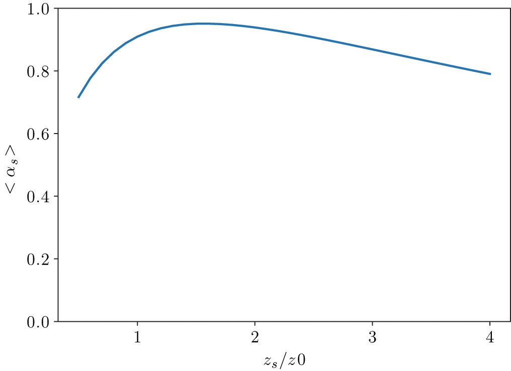
Figure 9.30 Diffuse field absorption for varying values of . Source: Alexander Peiffer.
9.3.6 Conclusions on Layer Formulation
The above derived transfer matrices are useful for the determination of transmission (and therefore also coupling) of large area junctions. Energy is removed from the reverberant field by absorption taking place at every reflection. The approximation of infinite layer is the more valid the larger the areas are. In any case this formulation is a powerful tool to derive properties of so-called acoustic treatments, layers of different materials that are used as noise control treatment in many applications.
9.4 Acoustic Absorber
Acoustic absorbers are used to reduce the noise levels in cavities and rooms. The task is to create a lay-up that maximizes the absorption in a specified frequency range with the least space and weight requirements. The target value is , because this leads to perfect matching at an angle of that contributes most to the diffuse absorption coefficient. We start with a simple absorber created by a single layer of fiber material. The next step will be a combined absorber consisting of a fiber absorber plus perforated sheet.
9.4.1 Single Fiber Layer
When placing an absorbing fiber layer in front of a rigid wall, the transfer matrix is connected to a rigid wall, meaning that in equation (9.96)
For the surface impedance this leads to
For first evaluation of our fiber material described in section 9.3.4, we use the fluid transfer matrix (9.106) with the material parameters from (9.107a)–(9.107)g. In figure 9.31 the impedance spectrum for is shown for materials of different thicknesses.

Figure 9.31 Perpendicular surface impedance of single fiber layer in front of a rigid wall. Source: Alexander Peiffer.
The reactance of the 20 cm layer shows a first resonance at but with no clear peak. The 10 cm version has a local maximum around the double frequency. As damping increases with frequency, the 10 cm resonance is weaker and does not reach zero reactance. When we consider equation (2.104), at higher frequency both layers coincide, because the high damping in the material prevents any feedback from reflected waves.
We see that zero reflection requires a real for normal incidence. So, the material shown before seems to be a performing fiber absorber, as resistance is near the impedance of air. In Figure 9.32 the absorption due to normal wave incidence is shown for both layers. The early resonance of the 20 cm layer leads to better performance at lower frequencies with a dip afterwards. At ω = 400s−1, there is weak absorption for the 10 cm layer, whereas the 20 cm layer provides already . However, a 20 cm layer requires a lot of space that is not always available. Thus, we look for an option to reduce the thickness but keep the low frequency performance.

Figure 9.32 Perpendicular surface absorption of a single fiber layer in front of a rigid wall. Source: Alexander Peiffer.
The low speed of sound in the fiber material leads to a large wavenumber in the fiber. The consequence is that even oblique waves are diffracted to the surface normal, and the angle dependence to the impedance is quite low. Thus, the normal and diffuse absorption are not that different (figure 9.33).
Figure 9.33 Diffuse absorption of a single layer in front of a rigid wall. Source: Alexander Peiffer.
9.4.2 Multiple Layer Absorbers
In many cases there is not enough space for large thickness absorbers available; or, the environment does not allow for porous materials, because the surface will be exposed to dirt and humidity. we must protect the absorber by a thin layer (thin and soft plates) or use perforate that can be cleaned.
9.4.3 Absorber with Perforate
A perforate with micro absorption may have a transfer impedance with resistance on the order of magnitude of air and with additional mass generated by the neck effect as described in section 9.1.7. This mass can be used to lower the resonance of the total system and therefore to reduce the thickness of the absorber.
The advantage of this concept is that we can separately tune the resistance of the front sheet to air and the thickness of fluid or fiber layer to create zero reactance. Let us assume that the layer generates a surface impedance of . The state vector is then given by
The state vector of the front layer follows from matrix multiplication with the limp layer transfer matrix
so the final surface impedance reads
This is why limb elements that are characterised by are well represented by a transfer impedance that simply adds to the backing impedance. Coming back to our design problem, we can select an air layer that provides zero reactance at thickness and choose a perforate with the matching resistivity. In Fuchs and Zha (1995) some micro-perforate absorbers with the desired quantities are given. We use the absorber of figure 6 of Fuchs and Zha and the parameters shown in Table 9.5.
Table 9.5 Absorbers with different perforate plates and constant surface porosity. Source: Fuchs and Zha (1995).
| Mesh | mm | mm | mm | mm | |
|---|---|---|---|---|---|
| 1 | 3.0 | 1.5 | 22.5 | 50 | 0.014 0 |
| 2 | 3.0 | 0.225 | 3.37 | 50 | 0.014 0 |
| 3 | 3.0 | 0.075 | 1.13 | 50 | 0.013 8 |
In figures 9.34 and 9.35 the resistance and reactance of the perforates are shown. One can recognize that the resistance of the second mesh fits best to our above condition for best absorption. The resistance of mesh 1 is too low and mesh 3 too high. Mesh 2 nearly meets the requirements over a large frequency range.

Figure 9.34 Transfer resistance of three different micro-perforates. Source: Alexander Peiffer.

Figure 9.35 Transfer reactance of three different micro-perforates. Source: Alexander Peiffer.
From the three reactance curves, we conclude that the high inertia from mesh 1 and 2 might reduce the frequency range of the absorber, because the reactance of the mesh is added to the reactance of the air spring as shown in Figure 9.35. A pure resistive absorber would have best absorption for ; with the mass effect, the resonance is lower. This is because the stiffness of the air spring sees the mass of the perforate, and the resonance frequency is reduced. In Figure 9.35 this can be seen by the intersection point of and .
The normal impedance of the full absorber is shown in Figure 9.36. The normal and diffuse field absorption is shown in figures 9.37 and 9.38. The result does not fit perfectly to Fuchs’ test results, but the global tendency and resonance frequency is well met.

Figure 9.36 Surface impedance of micro-perforate absorber. Source: Alexander Peiffer.

Figure 9.37 Normal incidence absorption of micro-perforate absorber. Source: Alexander Peiffer.

Figure 9.38 Diffuse field absorption of micro-perforate absorber. Source: Alexander Peiffer.
9.4.4 Single Degree of Freedom Liner
The micro-perforate absorber is a perfect candidate for building absorbers. In aerospace applications the absorber must withstand strong aerodynamic load, pressure, and heat. Thus, the perforate is fixed to a carrier structure. This is usually a honeycomb material made out of aluminium or aramid fiber paper (Figure 9.39). Such liners are used in the inlet section of turbo-fan nacelles but also inside engines in cold and hot streams. In these absorbers the waves cannot propagate in in-plane directions, and we must use the normal incidence impedance of an air layer as surface impedance of the honeycomb layer. This means we set the wave number in the -direction in equation (9.105) and neglect the volume fraction of the honeycomb wall material.

Figure 9.39 Single degree of freedom liner with (a) hard backing, (b) honeycomb core and (c) perforated sheet. Source: Alexander Peiffer.
With the configuration from Table 9.6, we get the transfer impedances as shown in figure 9.40. We see that the resistance condition and the resonance occur at the same frequency. In Figure 9.41 we see that the absorption is nearly 1 at a certain frequency band around this regime. This is acceptable, because in turbofan engines the absorption is optimized for specific tones in the engine. It must be noted that in real aircraft liner designs, the airflow must be considered, because the high Mach number current changes the neck correction (Hubbard and Acoustical Society of America, 1995).

Figure 9.40 Transfer resistance and reactance of liner perforate. Source: Alexander Peiffer.

Figure 9.41 Surface impedance and absorption of liner. Source: Alexander Peiffer.
Table 9.6 Aerospace liner set-up
| mm | mm | mm | mm | |
|---|---|---|---|---|
| 1.5 | 0.2 | 3 | 30 | 0.022 |
9.5 Acoustic Wall Constructions
9.5.1 Double Walls
Inspecting wall configurations that aim at high acoustic isolation at reasonable weight leads to the conclusion that many engineering systems are enhancing the acoustic isolation of a single wall by simply adding a second wall with some absorbing material in the middle. Examples are the interior lining in aircraft covering layers of glass fiber blankets (Peiffer et al., 2007, 2013), gypsum plasterboards in buildings, or mass-spring layers in the automotive industry used, for example, to increase the isolation of the firewall in cars.
The generic setup is shown in Figure 9.42. The walls consist of panels that may be considered as limp mass or plates. In both cases they are described by thin layer transfer equation (9.27) with different transfer impedances and

Figure 9.42 Double wall lay-up of panel–cavity–panel. Source: Alexander Peiffer.
The cavity or fluid layer is given by (9.106).
The transfer matrix of the full system is given by
In this case the result can be derived analytically and we get after some math
 (9.118)
Applying equation (9.109) gives the transmission coefficient for the double leaf configuration
 (9.119)
For low frequencies the wavelength in the double wall cavity is much larger than the thickness, and equation (9.118) can be simplified to
Thus, at low frequencies the layers are supposed to be stiffly connected.
9.5.1.1 Double Wall of Limp Mass
For further insight we use the ideal case of two limp mass layers with transfer impedance and . The fluid gap can be a fluid like air, other gases, or an equivalent fluid, hence . The double wall transmission loss reads with this assumption
 (9.121)
We can show that at low frequencies , eq. (9.121) gives the mass law of infinite single walls (8.96) with total mass . The same conclusion follows from (9.120) when we assume the mass transfer impedance . In figure 9.43 the transmission coefficients are shown for and . There is a first minimum of the transmission loss that is called the double wall resonance and will be dealt with later. Below this resonance the result coincides with the mass law curve of a single wall of the same total mass.

Figure 9.43 Transmission coefficient for plane waves transmission. Double wall of two limp layers of kg/m2 and air cavity of cm thickness. At the axis the resonance frequencies of perpendicular waves are denoted. Source: Alexander Peiffer.
In the regime above the double wall resonance, there are several dips that correspond to resonances of the cavity for , and the tangent in equation (9.121) becomes infinite. In other words the thickness of the cavity equals integer multiples of the half wavelength. The cavity resonances are denoted by in figure 9.43. When damping in the cavity is not too high (which is definitely the case for air), the anti-resonances for
lead to a decoupling and equation (9.121) is approximated for high frequencies by:
Note that high damping means a complex wavenumber and the condition cannot be met, and the above estimation is not valid. Writing the above expression as transmission loss, we see that above the double wall resonance, the single transmission loss of each wall is summed up, plus an extra term
The best use of available mass for high transmission loss is given for a distribution of two walls. This is the reason why double leaf constructions are the power weapons for acoustic isolation in many fields of technical acoustics.
However, at the resonances the isolation performance of the double wall can be low, lower than the mass law. Thus, the resonances must be reduced by damping in the cavity, and we must understand what determines the frequency of the double wall resonance. This can be found by determining the minimum of the denominator of equation (9.121) as shown, for example, by Fahy (1985). We apply the transfer matrix expression (9.118). Perfect transmission is given when the transfer matrix becomes a unit-matrix, thus and . In general the thickness of a double wall is much smaller than the wavelength at low frequencies, so and we use and .
The diagonal components of (9.118) are, with
and are close to unity for typical wall dimensions. The approximation of reads
This matrix coefficient is zero at
 (9.126)
The result is the natural frequency of a spring with masses at both ends. The approximation corresponds to a massless spring. However, in double wall construction, the filling of a double wall is lightweight. Figure 9.44 shows the diffuse field transmission loss determined from angle integration. The cavity resonances are smeared out due to the integration but the double wall resonance is still visible.

Figure 9.44 Diffuse field transmission coefficient. Double wall of two limp layers of kg/m2 and air cavity of cm thickness. Source: Alexander Peiffer.
9.5.2 Limp Double Walls with Fiber
As the excellent performance of a double wall is partly compensated by the cavity or double wall resonances, those must be damped by absorbing material, and due to equation (9.122), the characteristic impedance should not be too high. The fiber material of section 9.3.4 is an appropriate candidate for such an application. The air of the double wall cavity is replaced by the fiber material by using the material data of the equivalent fluid. First, we see in Figure 9.45 that the double wall resonance is lower than in air. This results from the lower speed of sound in the fiber material. Second, the transmission loss is much higher than for the air filled cavity, and the notches due to the thickness resonances are not existing. This is a result of the high damping in the fiber material.

Figure 9.45 Transmission coefficient for plane waves transmission. Double wall of two limp layers of kg/m2 and fiber cavity of cm thickness. Source: Alexander Peiffer.
It must be kept in mind that this is infinite layer theory. Thus, the calculated transmission loss is slightly overestimated compared to real systems. Every wall must be connected to the other wall by mounts that jeopardize the high isolation; secondly, the finite size of panel and absorber is not taken into account as it is already shown for single walls in section 8.2.4.5. However, for a principle understanding of double wall phenomena, the infinite layer theory is excellent. In Chapters 10 and 11, we will see how the finite size can be considered.
9.5.3 Two Plates with Fiber
Large areas cannot be realized by limp heavy layers, because a certain stiffness is necessary to mechanically hold the plate. The consideration of bending stiffness is done by using the transfer impedance of plates (9.101) in equation (9.119). Figure 9.46 shows a similar shape as for the limp double wall with fiber material. In addition there are the coincidence peaks from the bending waves of the aluminium plates. It is clear that plate materials with similar coincidence frequencies should be avoided, so that only one plate coincides with the exciting or radiating fluid wave.

Figure 9.46 Transmission coefficient for plane wave transmission. Double wall of two aluminium plates of thicknesses 3 and 5 mm and fiber cavity of cm thickness. Source: Alexander Peiffer.
9.5.4 Conclusion on Double Walls
The results from Section 9.5 are some of the most relevant results for passive noise control and acoustic isolation of enclosures or walls. Therefore, we recapitulate the most important conclusions.
Below the double wall resonance, the system behaves as a single wall of the same mass with no benefit regarding noise isolation. Above the double wall resonance, the system performs much better, likely 20 dB and more, because the single transmission coefficients are multiplied and not added.
Thus, design rule number one is: Try to keep the double wall resonance as low as possible. For further details we introduce the reduced mass by
and the frequency is then given by
Weight is a critical parameter in most technical systems. So, we need the best mass distribution for given total mass per area . Let us assume that is the fraction of the total mass giving the first mass.
and the reduced mass reads for
The maximum is at so the lowest double wall frequency is given for a symmetric mass distribution. This ideal condition cannot always be achieved, because the main structure has to provide certain stability and is the heavy part of the wall, for example fuselage panels (Peiffer et al., 2013), walls of buildings, or the body-in-white of a car. In those cases the weight of the second wall is lower than for the main structure . In this case the reduced mass is approximated by

Figure 9.47 General shape of the double wall transmission and the relationship to main parameters. Source: Alexander Peiffer.
Thus, the light part determines the frequency. As a further consequence it does not make much sense to use a much heavier structure as the first structure, because the resonance is no longer efficiently decreased. So, rule number one under these constraints means to distribute the mass symmetrically if possible. If one wall structure is given, don’t use a mass that is much higher than the first leaf, because this will not be efficient.
For high frequencies the performance according to equation (9.122) is
that becomes also maximal at .
The next important parameters are the cavity thickness and stiffness, given by . Thus, a possible trade off can be space to weight. However, this can be difficult for lower frequencies, because the thickness can, for example, reach more than 15 cm in case of the first blade, passing the frequency of turbo-props around 100 Hz for fuselage noise control.
The stiffness of the centre cavity or layer can be reduced by using fiber material with low speed of sound, but this is partly compensated by the effective higher density. Double walls are also often realized by soft foams with Young’s modulus around kN/m2. Those systems are called mass-spring treatments. We should keep in mind that the lowest reasonable Young’s modulus is near 90 kN/m2, because this is the stiffness per area of the air spring in the material, as kN/m2.
Rule number two: The space between the layers must be damped. At least there must be some damping; more damping will further increase the performance, but not much. The necessity for damping depends on how much transmission is allowed near the double wall resonance.
Rule number three: Don’t forget the coincidence. If possible use wall properties that lead to different frequencies, or use a lining that is limp.2
To conclude, an efficient double wall system is designed by two panels of similar weight and thick space filled with soft and damped material. One remark concerns the impermeability of the walls. This must be guaranteed to exploit the advantages of double walls. Due the high performance of the total system, small leakages may have a tremendous effect. So, if leakage cannot be avoided due to technical reasons, eg. cable, ventilation, or pipe cut-outs, put special care on the design of sealing systems at those critical areas.
Bibliography
- Jean-F. Allard and Noureddine Atalla. Propagation of Sound in Porous Media. Wiley, second edition, 2009. ISBN 978-0-470-74661-5.
- Jean F. Allard, Michel Henry, Laurens Boeckx, Philippe Leclaire, and Walter Lauriks. Acoustical measurement of the shear modulus for thin porous layers. The Journal of the Acoustical Society of America, 117(4): 1737–1743, April 2005. ISSN 0001-4966.
- M. A. Biot. Generalized Theory of Acoustic Propagation in Porous Dissipative Media. The Journal of the Acoustical Society of America, 34(9A): 1254–1264, September 1962. ISSN 0001-4966.
- Yvan Champoux and Michael R. Stinson. On acoustical models for sound propagation in rigid frame porous materials and the influence of shape factors. The Journal of the Acoustical Society of America, 92(2): 1120–1131, August 1992. ISSN 0001-4966.
- Frank Fahy. Sound and Structural Vibration: Radiation, Transmission and Response. Academic Press, London, The United Kingdom, 1985. ISBN 0-12-247670-0.
- FreeFieldTechnologies. Actran 16.0 User’s Guide. Mont-Saint-Guibert, Belgium, two thousand, sixteenth edition, October 2015.
- H. V. Fuchs and X. Zha. Einsatz mikro-perforierter Platten als Schallabsorber mit inhärenter Dämpfung. Acta Acustica united with Acustica, 81(2): 107–116, March 1995.
- Kirill V. Horoshenkov, Alistair Hurrell, and Jean-Philippe Groby. A three-parameter analytical model for the acoustical properties of porous media. The Journal of the Acoustical Society of America, 145(4): 2512–2517, April 2019. ISSN 0001-4966.
- Harvey H. Hubbard and Acoustical Society of America, editors. Aeroacoustics of Flight Vehicles: Theory and Practice. Published for the Acoustical Society of America through the American Institute of Physics, Woodbury, NY, 1995. ISBN 978-1-56396-407-7 978-1-56396-404-6 978-1-56396-406-0.
- Finn Jacobsen. PROPAGATION OF SOUND WAVES IN DUCTS. Technical Note 31260, Technical University of Denmark, Lynby, Denmark, September 2011.
- Dah-You Maa. Potential of microperforated panel absorber. The Journal of the Acoustical Society of America, 104(5): 2861–2866, November 1998. ISSN 0001-4966.
- Fridolin P. Mechel, editor. Formulas of Acoustics. Springer, Berlin; New York, 2002. ISBN 978-3-540-42548-9.
- Clemens Moeser, Alexander Peiffer, Stephan Brühl, and Stephan Tewes. FEM Schalldurchgangsrechnungen einer Doppelwandstruktur. In Fortschritte der Akustik, pages 593–594, Dresden, Germany, March 2008.
- M. L. Munjal. Acoustics of Ducts and Mufflers with Application to Exhaust and Ventilation System Design. Wiley, New York, 1987. ISBN 978-0-471-84738-0.
- Raymond Panneton. Comments on the limp frame equivalent fluid model for porous media. The Journal of the Acoustical Society of America, 122(6): EL217–EL222, 2007.
- Alexander Peiffer, Stephan Tewes, and Stephan Brühl. SEA Modellierung von Doppelwandstrukturen. In Fortschritte der Akustik, Stuttgart, Germany, March 2007.
- Alexander Peiffer, Clemens Moeser, and Arno Röder. Transmission loss modelling of double wall structures using hybrid simulation. In Fortschritte Der Akustik, pages 1161–1162, Merano, March 2013.
- Allan D. Pierce. Acoustics - An Introduction to Its Physical Principles and Applications. Acoustical Society of America (ASA), Woodbury, New York 11797, U.S.A., one thousand, nine hundred eighty-ninth edition, 1991. ISBN 0-88318-612-8.
- Karin Tageman. Modelling of sound transmission through multilayered elements using the transfer matrix method. Master’s thesis, Chalmers University of Technology, Gothenburg, Sweden, 2013.
- Huiyu Xue. A combined finite element–stiffness equation transfer method for steady state vibration response analysis of structures. Journal of Sound and Vibration, 265(4): 783–793, August 2003. ISSN 0022-460X.
Notes
- 1 The third term corresponds to the moving mass in front of a piston as discussed in section 2.7.3.
- 2 This is why the lining is often called trim, because in historic aircraft the second wall was realized by a trimmed membrane