13.3.1 Transfer Path Analysis

The transfer path analysis (TPA) is based on the measurement of the frequency transfer function of vibroacoustic systems. Hence, the dynamics of the systems is reduced to specific points of interest: mount connection, passenger ear positions, or excited locations. This transfer function is measured for multiple inputs (forces, moments, and acoustic volume strength) and responses (acceleration, displacement, and pressure). A good overview about the history and state of the art can be found, for example, in (van der Seijs et al., 2016).

The system is subdivided into subsystems that are connected via specific point shaped connections so that the transfer functions of the main paths are included. Those transfer functions are similar to the matrix (1.198) as introduced in section 1.7.

Both response and excitation are measured. For structural excitation this is done with piezoelectric transducers that measure the force generated by impact hammers or shakers and accelerometers for the response. Instead of accelerometers a scanning laser vibrometer can be used. Acoustic sources with given source strength $\mathit{Q}$ are realized by special loudspeaker systems sometimes connected to long tubes in order to establish a point source. The pressure response is determined by microphones.

The determination of the transfer functions is performed using broadband signals (white noise, sweeps, or the given hammer impact history) and by applying equation (1.194). Hammer measurements are usually averaged over several impacts.

The transfer function of the subsystem is then inverted to get the stiffness or mobility matrix of the subsystems of interest. Especially this inversion is the critical point in TPA because noisy signals and test errors may lead to badly conditioned matrices and erroneous results. Many papers deal with methods to increase the robustness of this inversion by using pseudo inverses and additional reference sensors to create overdetermined systems.

In combination with an operational analysis, the TPA determines the forces occurring at the interface connections. From the forces and the local stiffness, the power input to the system can be calculated, and transfer paths are rated in terms of significance. The precision of these and power forces depends strongly on the quality of the matrix inversion and the test result in general.

When the systems become random, phase and magnitude of the system responses become uncertain. In this case the TPA can no longer be applied.

13.3.2 Experimental Modal Analysis

The mode shapes of structural or fluid systems can be measured directly. The tests and the related analysis methods are called experimental modal analysis(EMA). The system of interest is either equipped with a sufficient number of sensors to capture the modal shape and excited at one or a few excitation points. Instead, few response sensors and a large number of excitation positions can also be used. Due to reciprocity both methods provide the same result.

The are several methods to analyze measured frequency response functions and to extract the modal properties. A comprising overview about the existing methods is given by He and Fu (2001). The measured mode shapes can be used in modal frequency analysis similar to numerics, or the shapes are used as experimental reference. In this case the simulated modes are compared to the experimental shapes.

The major challenge is to estimate clean transfer functions for precise mode shapes, in particular for higher order modes. One advanced method is to estimate these functions by a best fit to a fraction of polynomial functions named PolyMAX parameter estimation (Peeters et al., 2004).

13.3.3 Correlation Between Test and Simulation

It is common practice that test and simulation results are compared based on point responses, e.g. pressure at driver’s ear from simulation and test. This might work for low frequencies and deterministic systems but may be misleading for complex systems. It is much better to compare the system responses for many positions distributed over this full system.

It does not make much sense to compare hundreds of response curves in one diagram. Thus, specific criteria are introduced to compare shapes, for example shapes of modes or frequency responses. Here, the most used criteria for mode comparison is given, the so called modal assurance criteria (MAC):

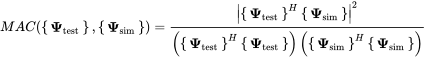  (13.1)

Under the condition of normal modes and perfect agreement the MAC is supposed to be orthogonal, hence $MAC=1$ for equal mode shapes and $MAC=0$ for different shapes. For the global agreement of the dynamic behavior the modal frequencies must also be equal.

The application of this criterion is state of the art in model updating methods and included in many test software packages. Nevertheless, there are many practical pitfalls. Note, that structural modes are mass normalized as given by equation (1.119) and that the mass matrix is usually not available in experimental modal analysis. So, for systems with very irregular system and mass distribution, this must be considered. This affects the orthogonality of the modes; thus, different modes don’t have zero MAC. See Allemang (2001) for more details. In addition the shape might be undersampled, meaning that the selected sensors are not dense enough to catch all details of the high frequency shapes.

There are several approaches besides engineering judgement to overcome such issues. One option is to check the so called AUTOMAC first. This is the MAC when the modes are correlated to themselves. If the result is the unit matrix, the selected test mesh and the mass distribution are supposed to be correct. A further issue is the case when modes have the same frequency and thus cannot be identified as distinct modes in the test. Obviously, only deterministic systems can be compared by this criterion.

When it comes to correlation of an SEA simulation with tests, things are getting more complicated. The SEA result is the average result of an ensemble of systems. Thus, curve comparison of single tests are reasonable when the systems are clearly random, as it is the case, for example, in the academic test cases of Chapter 10.

For the correlation of SEA models to tests, the system responses must be measured at many locations to get a good spatial average. Theoretically, even an ensemble of systems should be tested, which is not possible in most cases. Especially, single point response comparison are definitely no solution. However, when automatic test systems such as laser scanning systems or robots are used, a certain average can be achieved, and the comparison of physical units or the energy is possible. The investigation of the structure borne wave propagation along the aircraft fuselage in Chapter 12 is one example of this practice (Weineisen, 2014). A detailed correlation of the fuselage sidewall to SEA models is dealt with in Wang (2015).

13.3.4 Experimental or Virtual SEA

The experimental SEA can be considered as a transfer path analysis of random systems. The concept of virtual SEA is to measure the input power (from force and acceleration) at several excitation points on each subsystem and the velocity or pressure response on several locations of the connected and responding subsystems. The energy of such systems is estimated from (6.116) and (6.118). For the latter equation assumptions for the mass distribution must be made.

We start from the nonsymmetric version of the SEA equation (6.102), so the the modal density is not required. When we assume that the power introduced into the $n$th subsystem is given by ${\mathrm{\Pi }}_{\mathrm{i}\mathrm{n}}^{(n)}$ and the energy response of the $m$th subsystem due to this excitation is denoted by $E_{mn}$ we get the following equation system for three systems

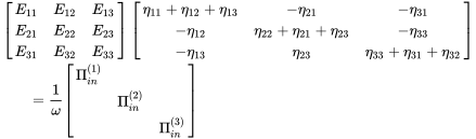  (13.2)

The subsystem energy is derived with (6.116) or (6.118). This can become a complicated task for irregular shapes and mass distribution, e.g. a ribbed plate of a fuselage panel (Bouhaj et al., 2017).

In equation (13.2) there are nine equations for nine parameters when we write the power load and energy matrices in one column. This system of equations is solved for ${\eta }_{ij}$. There are several investigations on experimental SEA, for example Lalor (1987), (1990), (1997), continued by the investigations on practical systems from Borello (2009), (2015)and Borello and Gagliardini (2007). Similar to the transfer path analysis, the determination of the coupling loss factors require an invertible matrix that is not always provided by tests. One key measure to overcome this is the method of averaging. Lalor proposed calculating the coupling loss factor from every measurement and average the coupling loss factors. Other authors average all excitation positions over one subsystem. Bouhaj et al. (2017) propose a statistical method to bring more robustness into the matrix inversion. In any case, virtual experimental SEA can be a promising tool to create SEA models from test data.

In addition the same method can be applied using FE simulations. In this case the introduced power and the energy estimation is determined from simulations. The biggest advantage here is, that the amount of sensors is nearly unlimited. The global analysis procedure is exactly the same. Such studies can be used to investigate, for example, very complicated junctions where no simplified equations for the radiation stiffness are available.

Note that the general decision how the substructuring is made is the duty of the experimentalist. Hence, also experimental SEA requires decisions about the SEA model set-up namely on the separation of the system into subsystems. This is further evidence for the fact that experimental people need theoretical knowledge.

13.4.1 Advances in SEA and Hybrid FEM/SEA Methods

Further reading on SEA is provided by Le Bot (2015) who introduces many aspects of the statistical concept of SEA and constitutes the link to statistical physics. Langley (2007), (2016)developed an extended version of the diffuse field reciprocity (7.19) based on a modal approach and for subsystems that don’t carry a perfectly diffuse wave field. An interesting field of research is the automatic recognition of components of a hybrid FEM/SEA model as developed by Langley and Kovalewski (2012).

Some research projects aimed at developing or collecting methods for the “mid frequency” range. One example is the Marie Curie project “MID-Frequency”– CAE-Methodologies for Mid-Frequency-Analysis in Vibration and Acoustics (Atak et al., 2012). A text book on current research in vibroacoustic simulation and many practical examples was edited by Hambric et al. (2016).

13.5.1 More Realistic Systems

In the initial chapters of this book we stayed with canonical and simple systems, such as homogenous plates and cavities. They were perfect for the exemplification of the method. Unfortunately, reality is neither canonical nor simple. Thus, a next step is to include more realistic but usually also complicated subsystems into the determination of modal density, wavenumber, and damping. Typical candidates are specific lay-ups, for example composite or sandwich plates. Integrated structures can be corrugated or beaded plates, rib-stiffened plates, or extruded profiles as shown in Chapter 12.

In many cases an analytical formulation of such materials or shapes does not make sense. The required equations may become more complicated and computationally even more demanding than numerical models. However, some more advanced descriptions of subsystems are available that can be managed with reasonable effort. Note that the thin shell is not correct for high frequencies, too. Here, thick plate theory must be applied, introduced, for example, in Cremer et al. (2005).

13.5.2 Anisotropic Material

All examples in this book are using isotropic materials, meaning that the mechanical or acoustical properties are independent from the orientation. The mechanical strength and superiority of carbon fiber or glass fiber reinforced plastics comes from the fact that highest strength is designed into the direction of the highest load. Hence, those materials must be anisotropic to fulfill this specification. Anisotropic materials are used in plates, shells, or beams. So, they are mostly used for example in plate theory.

13.5.3 Porous Elastic Material

In section 9.3.4 the limp fiber model was introduced, which is a useful description for porous material without frame dynamics. One reason for using this model was that the theory is not too complex. For some foam materials that are used in the automotive industry, for example as firewall mass-spring noise control treatment, the Biot (1962) model must be used. The consideration of such layers makes special layer formulations necessary plus interface conditions. The topic of porous materials is a research subject of its own and still an ongoing field especially in the experimental field. The book from Allard and Atalla (2009) gives a comprehensive treatment of this topic. There are many recent formulations (Horoshenkov et al., 2019; Lafarge et al., 1997) of the thermal and viscous dissipation during the wave propagation in the porous frame showing that the topic is still a field of basic research.

The simulation of coupled fluid structure models in combination with porous finite elements is still in the process of being implemented as standard procedure.

13.5.4 Composite Material

In section 3.7 we dealt with the in-plane forces (3.148) and moments (3.185). The linear laminate theory is well established in structural lightweight design and specific equations for bending and in-plane waves are elaborated, for example, in Baker and Scott (2016). Basically the behavior of a plate wave doesn’t change; the main difference to isotropic plates is that stiffness ratios between bending and in-plane strain can be different. In addition, the line moments and stresses can be coupled in case of unsymmetrical lay-ups.

13.5.5 Sandwich

More optimised plate structures in terms of lightweight design are sandwich plates that put most of the strength in the skin layer. The task of the very lightweight core material is to keep the distance between both skins. The dynamics of sandwich panels is special because the skin layers decouple from a certain frequency, so sandwich panels may be statically stiff and dynamically soft. This was shown by Kurtze and Watters (1959) and further detailed in (Moore and Lyon, 1991). This effect of decoupling depends mainly on the shear modulus of the core material. Note that due to the high stiffness and low weight, sandwich structures have the potential to become a vibroacoustic disaster because of a low and extended coincidence frequency range. However, by careful selection of the shear stiffness, this can be mitigated by dynamical decoupling.

In addition sandwich plates with heavy layers can constitute double walls due to the symmetric mode of wave propagation. In (Moore and Lyon, 1991) the transfer impedance for symmetric and nonsymmetric modes is given and can be used in the transfer matrix method to calculate the transmission loss.

13.5.6 Shell Theory

In this book we dealt with flat plates. In most engineering applications shells with curvature are used. There are several detailed textbooks dealing exclusively with shells of isotropic material, for example the books from Leissa (1993) and Ventsel and Krauthammer (2001). Special shapes often used in analytical SEA are cylindrical shells, also called singly curved, or spherical shells called doubly curved. A treatment of natural modes of cylindrical (and ribbed) shells is given by Szechenyi (1971). The work of Koval deals with the transmission loss and extends this treatment from cylinders of isotropic material (Koval, 1976) including pre-stress from internal pressure (aircraft fuselage) to composite cylinders.

13.5.7 Wave Finite Element Method (WFE)

The wave finite element method can be considered as a bridge between FEM and SEA in that sense that small FE models are used to calculate the parameters of SEA. Please note that this doesn’t mean the EFM or virtual SEA methods. The idea of the WFE is to take a representative unit cell and apply periodic boundary conditions. With these assumptions quantities such as speed of sound, wavenumber, and damping can be calculated from this unit cell.

This is a perfect method for simple systems as plates (Manconi et al., 2013) but especially for periodic systems such as rib-stiffened shells or extruded profiles (Cotoni et al., 2008; Orrenius et al., 2014).

In addition the WFE can be extended to the calculation of coupling loss factors as shown by Mitrou et al. (2017). This further opens the path to a systematic derivation of the coupling loss factor.

13.5.8 The High Frequency Limit

In section 6.3.1.5 it was shown that there is an upper limit for SEA. This is the case when the dissipation along the wave path is so large that a diffuse field cannot exist, because the waves are damped out and reverberation is not possible. The frequency limit for systems with the maximum length $L$ with this condition is

  (13.3)

This is the domain of methods that include the energy distribution in the systems. One option to take care of this is ray tracing, also called geometrical acoustics, as presented in (Pierce, 1991; Kuttruff, 2014). Examples for the application of ray tracing in the SEA context are presented by Gardner and Macarios (2014).

A different approach is introduced by Tanner. He developed an element based ray tracing method called dynamic energy analysis (DEA). In Tanner et al. (2012) the method is applied to plate systems.

Bibliography

- Jean-F. Allard and Noureddine Atalla. Propagation of Sound in Porous Media. Wiley, second edition, 2009. ISBN 978-0-470-74661-5.
- Randall J. Allemang. The Modal Assurance Criterion (MAC): Twenty Years of Use and Abuse. In Proceedings, 2001.
- Onur Atak, Bert Pluymers, Wim Desmet, and Katholieke Universiteit te Leuven (1970-). MID-Frequency- CAE Methodologies for MID-Frequency Analysis in Vibration and Acoustics. 2012. ISBN 978-94-6018-523-6.
- A. A. Baker and Murray L. Scott, editors. Composite Materials for Aircraft Structures. AIAA Education Series. AIAA/American Institute of Aeronautics and Astronautics, Inc, Reston, Virginia, third edition, 2016. ISBN 978-1-62410-326-1.
- M. A. Biot. Generalized Theory of Acoustic Propagation in Porous Dissipative Media. The Journal of the Acoustical Society of America, 34(9A): 1254–1264, September 1962. ISSN 0001-4966.
- Gerard Borello. Analysis of Vibroacoustic Systems using Virtual SEA, June 2009.
- Gerard Borello. SEA+ for Aerospace Applications, 2015.
- Gerard Borello and L. Gagliardini. Virtual SEA: Towards an industrial process. SAE Technical Paper, 2007-0123-02, 2007.
- M. Bouhaj, O. von Estorff, and A. Peiffer. An approach for the assessment of the statistical aspects of the SEA coupling loss factors and the vibrational energy transmission in complex aircraft structures: Experimental investigation and methods benchmark. Journal of Sound and Vibration, 403: 152–172, September 2017. ISSN 0022460X.
- V. Cotoni, R.S. Langley, and P.J. Shorter. A statistical energy analysis subsystem formulation using finite element and periodic structure theory. Journal of Sound and Vibration, 318(4-5): 1077–1108, December 2008. ISSN 0022460X.
- Lothar Cremer, Manfred Heckl, and Björn Petersson. Structure-Borne Sound: Structural Vibrations and Sound Radiation at Audio Frequencies. Springer Verlag, Berlin, Germany, 3rd edition, December 2005. ISBN 978-3-540-26514-6.
- Bryce Gardner and Tiago Macarios. Combining Ray Tracing and SEA to Predict Speech Transmissibility. In Proceedings 8th International Styrian Noise, Vibratoin & Harshness Congress : The European Noise Conference, June 2014.
- Stephen A. Hambric, S. H. Sung, and D. J. Nefske, editors. Engineering Vibroacoustic Analysis: Methods and Applications. Wiley, Chichester, West Sussex, United Kingdom, 2016. ISBN 978-1-119-95344-9.
- Jimin He and Zhi-Fang Fu. Modal Analysis. Butterworth-Heinemann, Oxford; Boston, 2001. ISBN 978-0-7506-5079-3.
- Kirill V. Horoshenkov, Alistair Hurrell, and Jean-Philippe Groby. A three-parameter analytical model for the acoustical properties of porous media. The Journal of the Acoustical Society of America, 145 (4): 2512–2517, April 2019. ISSN 0001-4966.
- L.R. Koval. On sound transmission into a thin cylindrical shell under “flight conditions”. Journal of Sound and Vibration, 48 (2): 265–275, September 1976. ISSN 0022460X.
- G. Kurtze and B. G. Watters. New Wall Design for High Transmission Loss or High Damping. The Journal of the Acoustical Society of America, 31 (6): 739–748, June 1959. ISSN 0001-4966.
- Heinrich Kuttruff. Room Acoustics, Fifth Edition. 2014. ISBN 978-1-4822-6645-0 978-0-203-87637-4.
- Denis Lafarge, Pavel Lemarinier, Jean F. Allard, and Viggo Tarnow. Dynamic compressibility of air in porous structures at audible frequencies. The Journal of the Acoustical Society of America, 102(4): 1995–2006, October 1997. ISSN 0001-4966.
- N. Lalor. The Measurement of SEA Loss Factors on a fully assembled Structure. Technical Report ISVR Technical Report Np. 150, Southampton, U.K, August 1987.
- N. Lalor. Practical Considerations for the Measurement of Internal and Coupling Loss Factors on Complex Structures. Technical Report ISVR Technical Report Np. 182, Southampton, U.K, June 1990.
- N. Lalor. The practical implementation of SEA. In Proceedings of the IUTAM Symposium, pages 257–268, Kluwer Academic Publishers. Southampton, U.K, July 1997.
- R. S. Langley. On the diffuse field reciprocity relationship and vibrational energy variance in a random subsystem at high frequencies. The Journal of the Acoustical Society of America, 121(2): 913–921, 2007.
- Robin S. Langley and Alice Kovalewski. Automatic recognition of the components of a hybrid fe-sea model from a finite element model. In Proceedings NOVEM 2012, page 11, Sorrento, Italy, April 2012.
- R.S. Langley. On the statistical properties of random causal frequency response functions. Journal of Sound and Vibration, 361: 159–175, January 2016. ISSN 0022460X.
- A. Le Bot. Foundation of Statistical Energy Analysis in Vibroacoustics. Oxford University Press, Oxford, United Kingdom; New York, NY, first edition, 2015. ISBN 978-0-19-872923-5.
- Arthur W. Leissa. Vibration of Shells. American Inst. of Physics, Woodbury, NY, 1993. ISBN 978-1-56396-293-6.
- B.R. Mace. Statistical energy analysis: Coupling loss factors, indirect coupling and system modes. Journal of Sound and Vibration, 279(1–2): 141–170, January 2005. ISSN 0022-460X.
- Elisabetta Manconi, Brian R. Mace, and Rinaldo Garziera. The loss-factor of pre-stressed laminated curved panels and cylinders using a wave and finite element method. Journal of Sound and Vibration, 332(7):1704–1711, 2013. ISSN 0022-460X.
- Giannoula Mitrou, Neil Ferguson, and Jamil Renno. Wave transmission through two-dimensional structures by the hybrid FE/WFE approach. Journal of Sound and Vibration, 389: 484–501, February 2017. ISSN 0022460X.
- J. A. Moore and R. H. Lyon. Sound transmission loss characteristics of sandwich panel constructions. The Journal of the Acoustical Society of America, 89(2): 777–791, February 1991. ISSN 0001-4966.
- Ulf Orrenius, Hao Liu, Andrew Wareing, Svante Finnveden, and Vincent Cotoni. Wave modelling in predictive vibro-acoustics: Applications to rail vehicles and aircraft. Wave Motion, 51(4): 635–649, June 2014. ISSN 01652125.
- Bart Peeters, Herman Van der Auwerer, Patrick Guillaume, and Jan Leuridan. The PolyMAX frequency-domain method: A new standard for modal parameter estimation? Shock and Vibration, 11: 395–409, 2004. ISSN 1070-9622/04.
- Allan D. Pierce. Acoustics - An Introduction to Its Physical Principles and Applications. Acoustical Society of America (ASA), Woodbury, New York 11797,U.S.A, one thousand, nine hundred eighty-ninth edition, 1991. ISBN 0-88318-612-8.
- P. J. Shorter. Combining Finite Elements and Statistical Energy Analysis. PhD thesis, University of Auckland, Aucklang, Newzealand, July 1998.
- E. Szechenyi. Approximate methods for the determination of the natural frequencies of stiffened and curved plates. Journal of Sound and Vibration, 14(3): 401–418, 1971.
- Gregor Tanner, David J. Chappell, Dominik Löchel, and N. Sondergard. A DEA approach for solving multi-mode large scale vibro-acoustic wave problems in the mid-to-high frequency regime. In Proceedings ISMA 2012, Leuven, Belgium, September 2012.
- Stephan Tewes and Alexander Peiffer. EFM-Modellierung einer Flugzeugdoppelwandstruktur. In Fortschritte der Akustik, pages 903–904, Stuttgart, March 2007.
- Maarten V. van der Seijs, Dennis de Klerk, and Daniel J. Rixen. General framework for transfer path analysis: History, theory and classification of techniques. Mechanical Systems and Signal Processing, 68–69: 217–244, February 2016. ISSN 08883270.
- Eduard Ventsel and Theodor Krauthammer. Thin Plates and Shells : Theory: Analysis, and Applications. CRC Press, August 2001. ISBN 978-0-8247-0575-6.
- Zhiyi Wang. Correlation between SEA Simulation and Test Results for a Double Wall Structure. Master’s thesis, TU-München, München, Germany, June 2015.
- Christian Weineisen. Modellierung einer Flugzeugstruktur mit der Statistischen-Energieanalyse. Master’s thesis, Technische Universität München (TUM), München, Germany, March 2014.