
7
Coupled Systems
When systems of similar physics are connected, the situation is relatively simple. The degrees of freedom of the coupling zone are shared, and the state variables, for example pressure and displacement, are equal. The situation changes for coupled deterministic systems of different wave types and physics. Here, conditions must be defined that link, for example, the pressure of one subsystem to the displacements of the other subsystem. The zone where the coupling dynamics takes place is called a junction.
However, simulating sound and vibration propagation in realistic systems means coupling systems of different types of wave propagation and different topology. This can be, for example, a fluid cavity that is connected to several plates surrounding it or a beam that is connected to other beams or plates. Hence, simulating the coupling dynamics can become a complicated task even for pure deterministic subsystems. However, the dynamics can be finally described by a large set of equations of motion with different degrees of freedom.
When random subsystems are connected, the description becomes more complicated. How can the coupling physics between random subsystems be described? If the state of random systems is given by energy, the power flow between the systems must be determined, given by the so-called coupling loss factor.
As shown in section 6.1, the boundary load of random systems is defined by a cross spectral density function that acts on the junction. In the junction itself, the dynamics is deterministic in the sense that the physics of the wave transmission through the connection is described in detail by deterministic equations of wave transmission. Thus, a junction between random systems must also be deterministic in order to catch the physics of wave transmission correctly.
A practical example for this can be two acoustic spaces or rooms connected by a thin wall or a window. In order to derive the energy exchange between the two spaces we must know precisely the wave behavior of this wall. In classical SEA literature, these phenomena are explained by wave transmission processes.
Here, we will apply the hybrid theory from Shorter and Langley (2005) and derive the link to the classical approaches. The advantage of Shorter’s hybrid approach is that it allows for systematic and logical derivation of SEA theory and coupling loss factors.
Hereinafter, deterministic and random systems are called FEM-systems and SEA-systems, respectively. The acronym FEM is selected because deterministic systems are usually modelled by finite element methods. In this chapter, we will deal with the connection of all these different systems.
7.1 Deterministic Subsystems and their Degrees of Freedom
In previous sections, we used continuous coordinates for the description of continuous systems. They are necessary, because quantities such as wave number, speed of sound etc. are derived based on continuous equations. In practical vibroacoustics, deterministic systems are rarely described by continuous coordinates but discrete coordinates. Nearly every geometry, set-up, and material configuration can be approximated by a discrete mesh. There exist a variety of tools and methods to simulate the dynamics of discrete systems. The maturity of commercial FEM software allows for the simulation of large and complex structures with several millions of degrees of freedom. In addition, other disciplines in the design process of vibroacoustic systems such as crash performance, statics, or dynamics also require finite element (FE) models. Hence, FE-models are usually automatically available early in the design process.
Therefore, it is reasonable to rely on FE-models for the deterministic part. We use the generalized degrees of freedom for the displacement denoted by
7.2 Coupling Deterministic Systems
When deterministic systems of similar natures are coupled, the joint degrees of freedom of both subsystems are the same. For example, a mechanical subsystem (1) as shown in Figure 7.1 can be described by the dynamic stiffness matrix
 (7.1)
(7.1)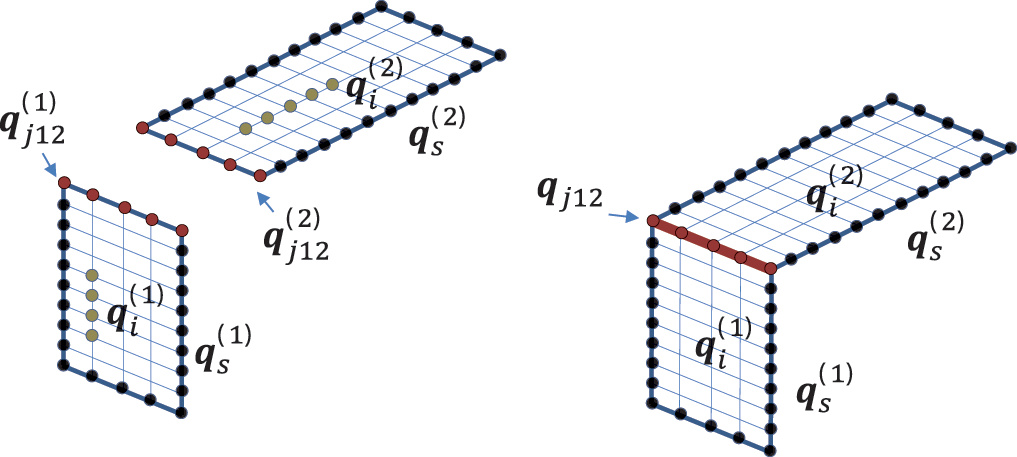
Figure 7.1 Internal, surface, and joint nodes of deterministic FEM systems. Source: Alexander Peiffer.
The expression external is motivated by the fact that these are the degrees of freedom that can be potentially excited by external forces. When creating a simulation strategy for a vibroacoustic system, it is helpful to consider the potential subsystem configuration from the very beginning and to identify which degrees of freedom are inner, external, or junction degrees of freedom. When doing so we always have the deterministic equations in the appropriate form.
When dealing with such system matrices it may be useful to get rid of the internal degrees of freedom and focus on the external or junction degrees of freedom. For outlining this procedure, junction and external degrees of freedom are denoted as outer degrees of freedom by a common subscript
Due to the fact that no external forces
Entering this in the lower part gives the stiffness matrix exclusively for the outer degrees of freedom.
This process is called condensation. It is of general importance to clearly define and handle the required degrees of freedom when dealing with vibroacoustic problems. The inner and outer degrees of freedom shall always be clearly differentiated.
A convention is required to sort these multiple definitions of degrees of freedom. According to the convention in the sections before, we use a subsystem superscript
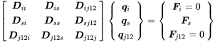
Now, let us assume that we have two subsystems as shown in Figure 7.1 on the right hand side. With these conventions, the stiffness matrix of the full deterministic system can be arranged in such a way that we have block matrices in the total matrix.
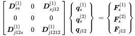
Using the reduced matrix from Equation (7.4) in order to get rid of the inner degree of freedoms we can write for subsystem 1 and 2:
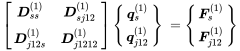 (7.5)
(7.5)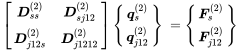 (7.6)
(7.6)Supposing the joint degrees of freedom are equal
 (7.7)
(7.7)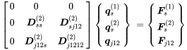 (7.8)
(7.8)Summing both matrices and integrating them into one global matrix reads:
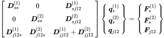 (7.9)
(7.9)The above exercise can be performed for any number of subsystem connections. This process might look somehow academical, but it has a very practical background. As discussed above, large engineering systems consist of many different subsystems. When putting subsystems together for a large system set-up the stiffness matrices must be added under consideration of the correct degrees of freedom.
As mentioned above the degrees of freedom of connections or junctions are always deterministic. Thus, the shared degrees of freedom denote the connection of both SEA and FEM-systems. They are the glue for all the subsystems independent from the fact of whether they are random or deterministic.
7.2.1 Fluid Subsystems
All the derived expressions from the section introduction can be transferred to cavities by exchanging
Acoustic or fluid matrices are denoted by the extra subscript a.
7.2.2 Fluid Structure Coupling
Whereas the coupling of pure structural or acoustic systems is well defined by shared degrees of freedom the situation is different for the coupling of fluid and structure. This is not a general problem. It comes from the fact that different quantities are used as degrees of freedom, the displacement for structures and the pressure (or velocity potential) for fluid waves. There are implementations that use the displacement as degree of freedom in fluid waves, which makes the coupling formulation easier but leads to other drawbacks. However, we have already defined the coupling and boundary condition when we derived the pressure–velocity relationship for acoustic waves with equation (2.35). The link to the displacement follows directly from
At structure surfaces this concerns only the normal vector. From this coupling condition, the finite element equations of combined fluid and structure systems are given by
as described in detail, for example, by Davidsson (2004).
7.2.3 Deterministic Systems Coupled to the Free Field
Technical systems are usually embodied in an exterior fluid. Thus, the vibrating systems that are connected to the surroundings radiate waves to the exterior. Usually, the simulation of radiation to the exterior is performed by boundary element analysis, but there are simpler and faster approximations that will be given in section 8.2.3. Technically, this means defining a radiation stiffness matrix that considers only the outer degrees of freedom. The physical interpretation of this is that every locally radiating element surface excites an acoustic pressure field. This pressure field leads to a force acting on the element itself and all others. Adding up all elements leads to the free field radiation stiffness.
In addition we have shown that the surface dynamics of random systems is given by free field dynamics when the modal overlap factor is high enough. For an ensemble average of uncertain systems this occurs even earlier when the system is dynamically complex. Thus, for the theory of coupling random systems, it is useful to elaborate the effect of semi infinite or finite systems on deterministic systems.
Imagine a deterministic system as shown in Figure 7.2. The FEM system in the middle is system

Figure 7.2 Deterministic system connected to two semi infinite systems. Source: Alexander Peiffer.
The free field stiffness is defined exclusively for the connected degrees of freedom. Consider a deterministic system connected to a free field as shown in Figure 7.2. The free field stiffnesses
 (7.13)
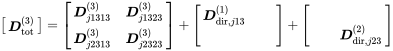
In order to keep the equations readable, we assume that the correct degrees of freedom are selected automatically. With this convention, the above definition of the total matrix reads
Here
This total stiffness combines the dynamics of the deterministic system and connected SEA systems. In the following, we will make use of this fact first in the context of coupling loss factors. For this derivation, we neglect excitation at the deterministic system except the reverberant load from the diffuse wave fields. Finally, the general form of Equation (7.15) for the total stiffness reads
7.3 Coupling Random Systems
The usual approach in classical SEA literature derives the coupling between random systems by application of wave scattering at the junctions or considerations based on reciprocity and excitation exactly at the junction. Here, we would like to apply the systematic approach by applying the diffuse field reciprocity relationship and the fact that the dynamics of every junction is determined by the total stiffness matrix.
In Chapter 6 we have shown that the expected value of stiffness of an ensemble of random systems is equal to the free field radiation stiffness because of the high dynamical complexity that does not allow for coherent reflection. Hence, the dynamic stiffness matrix of a random subsystem can be replaced by the free field direct radiation stiffness for the ensemble of random systems.
The impact of the random systems connected to the deterministic one is that each SEA system adds its free field radiation stiffness to the connected degrees of freedom of the deterministic system. Thus, the ensemble average dynamics of a deterministic system connected to several random systems can be described by the total stiffness matrix.
Finally, we have defined the impact of random subsystems on the deterministic system. Note that the ensemble mean works as a filter that extracts the deterministic part of the equations of motion.
The next step is the determination of the load generated by reverberant fields irradiating the junctions. The cross spectral density of this load is given by the reciprocity relationship between the direct field radiation and the reverberant loading. Shorter and Langley (2005a) have proven this diffuse field reciprocity relationship for arbitrary diffuse fields. We will not go into the details of this quite complex proof and present the final result for stiffness and impedance
What is the use of those relationships? They allow for the determination of random systems load at the boundaries just from energy, modal density and the free field radiation stiffness. Thus, for the simulation of the energy exchange between random systems they are an excellent foundation. The dynamics of a junction is determined by the free field radiation properties of the connected SEA systems and the load coming from the reverberant fields. With the presence of a deterministic system in the junction the dynamic stiffness of the FEM system must be added.
In Figure 7.3 the configuration is shown with direct and reverberant fields. Due to the connection to the random systems, the total stiffness is the sum of the dynamic stiffness of the deterministic system plus the two free field radiation stiffness matrices as in Equation (7.18).


Figure 7.3 Random subsystem exciting the deterministic connection in between (LHS) or deterministic junction only (RHS). Source: Alexander Peiffer.
On the right hand side of the Figure 7.3, there is no deterministic system in the connection of both random fields. In this case the junction boundary is considered as deterministic, and the related stiffness matrix is only the sum of the free field radiation stiffness of the connected subsystems.
7.3.1 Power Input to System
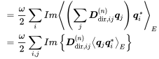
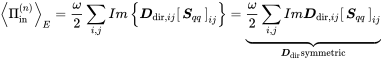
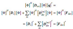
Random load excitation is given by the cross spectral density function. When we replace the system response matrix by the inverse of the total stiffness matrix
The cross spectral density of a stochastic load is hermitian; in case of diffuse fields it is a real matrix, and for symmetric radiation stiffness also symmetric. The cross spectral density matrix of the reverberant field can be replaced using the diffuse field reciprocity relationship (7.19)
This is the cross spectral density response of the FEM system of the junction degrees of freedom to the reverberant field with energy

Figure 7.4 Power flow from reverberant field (m) into system (n). Source: Alexander Peiffer.
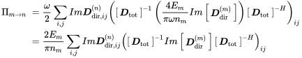
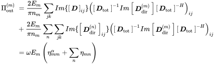
7.3.1.1 Power Radiated from Random Displacement
For the calculation of the power that is radiated into the
With the force
 (7.23)
When the stiffness matrix coordinates are a real based system the matrix is symmetric (Langley, 2007). In this case and only then, the hermitian cross spectral matrix can be factored out. This form is given in Shorter et al. (2005) under the assumption of symmetric stiffness matrices. In matrix notation we get
 (7.24)
with the cross spectral matrix (7.22), and by compiling all the information from the above considerations, we get the coupling loss factor in the hybrid formulation. From the energy power relationship (6.97) and the radiated power
 (7.25)
follows the coupling loss factor
- The free field radiation stiffness of the connected subsystems.
- The modal density of the source system.
- The dynamic stiffness matrix of the deterministic component of the junction.
In case of direct connection of random systems, the last item is neglected. When we now assume that there are several subsystems
with
7.3.2 Power Leaving the
The power loss in this section must not be confused with the internal power losses due to dissipation in wave propagation or absorption at the (random) boundaries. In previous sections and especially in Equation (7.27), we dealt with the power input from all neighbor systems. In contrast to this we deal here with the losses due to random load excitation at the junction and the dissipation in the deterministic part of the junctions plus the radiation to the connected systems. Thus, we replace the radiation stiffness in (7.24) by the total stiffness
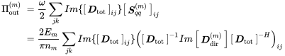 (7.28)
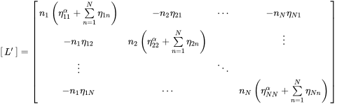
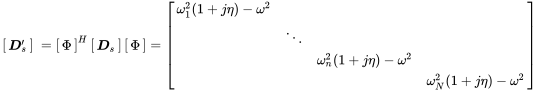
Introducing the detailed expression of the imaginary part of the total stiffness matrix
and entering it into (7.28) provides
 (7.30)
The right hand side of the above equation is the sum of all power leaving the
For a non-dispersive deterministic system the imaginary part of the dynamic stiffness matrix is zero and thus
However, the dissipation due to field and (random) boundary absorption is still given by
and we compile all expressions to1
With the above equations we can calculate all required coefficients for the SEA-matrix (6.113).
7.3.2.1 Assembling the Hybrid SEA Matrix
In Figure 7.5 the power components of the
- power input from external sources, e.g. forces, volume sources radiated into the system via the direct field.
- power input from surrounding SEA subsystems.
- power loss into the surrounding SEA subsystems and dissipation in the FEM subsystem due to interaction of the reverberant field with the junctions.
- power loss due to field dissipation and absorption at random boundaries.

Figure 7.5 Power balance of random subsystem connected to deterministic boundary and system. Source: Alexander Peiffer.
Setting up the power balance
and assembling all contributions leads to the same form as in Equation (6.113)
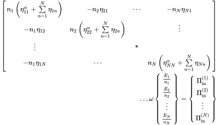 (7.34)
or
 (7.35)
7.3.3 Some Remarks on SEA Modelling
Before we get into detailed SEA models it is time to make some remarks. In the preceding sections we discussed the diffuse wave field model to describe random systems. In this chapter we presented the numerical toolbox to determine the exchange of power between diffuse reverberant fields. So, we are totally aware of the practical simplicity but also the restrictions of the diffuse wave field model. Imagine a system with many random subsystems – each of them must fulfill these restrictions. Imagine now in addition that we model the power flow through a cascade of such random systems because we have to model a system of connected plates. In every step of power flow from one system to the other, we will make an error, so consequently when applying SEA to this configuration the system must be really complex.
So, how can this dilemma be overcome? First, try to avoid small subsystems and cascades of subsystems in major paths of power flow. In other words try to model these parts by deterministic methods.
Second, in many cases a subsystem does not only transport acoustic energy via reverberant fields, but very often there is a forced motion of the subsystem. In the modal approach this corresponds to excitation of modes out of their resonant frequency. In the SEA language this path of indirect transfer is called the indirect or non-resonant path. We will later use the hybrid junction description in modal coordinates to clarify this phenomena.
And last but not least, we can correct the reverberant field assumption by methods of geometrical acoustics. This is standard in room acoustics due to the historical application of ray tracing methods in concert hall design or the prediction of large acoustic environments such as work shops or sporting event areas.
7.4 Hybrid FEM/SEA Method
Until now we have seen deterministic and random approaches to describe subsystems. When we dealt with single systems, we derived the criteria for how to separate the FEM from the SEA world normally at one specific frequency determined by Helmholtz number, dimension, and modal overlap. Real engineering systems consist of many such subsystems, and this specific frequency is different for each subsystem. Thus, it may happen that there are random and deterministic subsystems in one global system. This dilemma is called the mid-frequency problem and motivated the creation of the hybrid FEM/SEA method that combines both approaches in one set-up. In the preceding sections and the chapters before we have dealt with all means that are required to set-up the hybrid method, especially by including FEM components into the calculation of coupling loss factors. The FEM part was considered as part of a junction and an illustrative derivation of the coupling loss factor.
However, we did not include the FEM part in the global system context and did not include excitation of FEM degrees of freedom. Therefore, the hybrid FEM/SEA theory is introduced here again in a more general way.
In Figure 7.6 a generic set-up of of potentially three subsystems is shown. When defining a model of this configuration for the full audible frequency range from

Figure 7.6 Subsystem configuration over frequency. Source: Alexander Peiffer.
At low frequencies (case 1) the full set-up is modelled by FEM denoted by a mesh presentation of all subsystems. With increasing frequency the first subsystem becomes random (case 2), and now we must couple the reduced FEM system to the new SEA subsystem. Further increase in frequency (case 3) makes an additional component switch to random behavior, and the middle system must be considered in the junction formulation as defined by Equation (7.27). For even higher frequencies a full SEA (case 4) configuration may be required involving only pure SEA junctions, meaning that the total stiffness of (7.27) contains only the radiation stiffness terms.
The consequence is that we must apply both modelling principles in one model, with full flexibility if we would like to avoid creating several different models for the full frequency range as shown, for example, in Peiffer et al. (2013) and in section 12.2.3. However, Shorter and Langley (2005) have formulated this principle. We have already derived the components of this theory to explain the ideas of hybrid modelling, and we will extend this by deterministic and random excitation of the FEM subsystems.
7.4.1 Combining SEA and FEM Subsystems
In Figure 7.7 a generic FEM subsystem that is connected to several SEA systems is shown. The dynamics of the FEM part is defined by a matrix equation as shown for example in (5.1) and given by

Figure 7.7 Separation of a hybrid FEM/SEA system into FEM and SEA parts. Source: Alexander Peiffer.
here still considered as a deterministic matrix.
There can be excitation by external forces (deterministic and random) and reverberant fields. The sum of all external forces
is separated for practical reasons into the following components:
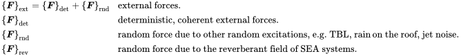
The ensemble average of the two forces with random character is zero
Putting the above loads and the stiffness matrices together gives:
This combination of matrices and excitation vectors must be reduced and separated into the FEM and the SEA part. We think of an ensemble of subsystems that is averaged to filter both components. In Figure 7.8 this filtering procedure is depicted. The mean value extracts the FEM components of the system; the expected value of the cross spectral density transforms the random systems into SEA components and keeps the deterministic system (for the coupling).

Figure 7.8 Application of ensemble averaging to a complex system. Source: Alexander Peiffer.
7.4.1.1 Ensemble Average of Linear State Variable
We start with the ensemble average of the equation of motion (7.38). On the left hand side the SEA matrix is replaced by the free field radiation stiffness because the ensemble average of random systems stiffness is equal to the free field radiation stiffness
and the ensemble average of the full equation reads, using the zero average of the random forces:
Thus, for the deterministic calculation the only impact of the SEA systems is the contact impedance, given by the free field radiation stiffness as illustrated on the left hand side of Figure 7.9. This reponse will lead to a power input into the reverberant fields of the SEA subsystems, but this is not considered in the deterministic response because of its non-coherent character and zero mean response.

Figure 7.9 Remaining expressions after ensemble averaging of all systems. Source: Alexander Peiffer.
7.4.1.2 Ensemble Average of Cross Spectral Density

Figure 7.10 Remaining expressions after ensemble averaging of cross spectral density. Source: Alexander Peiffer.
The cross spectral density is targeting the random part. From section 1.7.2 we know that the response to random loads requires the application of cross spectral density. Starting from the inverted (7.38) and neglecting the deterministic part
and using the expected value expression for the cross spectral density 1.205 we get
with
where the reverberant force term can be replaced by the diffuse field reciprocity expression
Equation (7.43) allows the calculation of an FEM subsystem response connected to several SEA subsystems and excited by random loads. According to our nomenclature we have to keep in mind that each subsystem is connected to specific degrees of freedom when we apply (7.43).
For practical reasons we make some further definitions. Usually, the FEM system is connected to several SEA systems.

Figure 7.11 The two effects of a SEA system on a connected FEM subsystem. Source: Alexander Peiffer.
In the discussion of section 7.3, the derivation was applied to FEM systems that are in the junction context. Here, Equation (7.13) is applied to the full FEM subsystem meaning that every SEA subsystem adds a free field radiation stiffness to the remaining dynamic stiffness.
Note that we must keep in mind the related degrees of freedom and the fact that the matrix
7.4.1.3 Integration of FEM into the SEA Power Flow

Figure 7.12 Remaining expressions for SEA power balance in the hybrid system configuration. Source: Alexander Peiffer.
This step was already dealt with in section 7.3 by using the deterministic formulation of the junction dynamics. Now, the (remaining) FEM system is given by all junctions and the deterministic systems. The SEA subsystems are modelled by the power flow Equation (7.34). The properties of the FEM subsystem are included in the total stiffness matrix
7.4.2 Work Flow of Hybrid Simulation

Figure 7.13 Workflow of hybrid simulation. Source: Alexander Peiffer.
The above derivation includes all steps of a workflow to calculate the dynamic response of deterministic and random subsystem over the full frequency range. Roughly speaking the workflow follows the above subsections 7.4.1.1 to 7.4.1.3. For reasons of simplicity the workflow is presented for one frequency domain with one subsystem configuration. That means we have already determined which subsystem is modelled as FEM and which one is considered as SEA. In later applications this decision has to be made for every frequency.
7.4.2.1 Setting up the System Configuration
The first step in hybrid modelling is the determination of the global configuration of FEM and SEA subsystems and the identification of junction areas or the specific degrees of freedom of the junction areas.
FEM1 Set up the combined discrete equations of motion of FEM subsystems according to Equation (7.12).
SEA1 Set up the properties of all SEA subsystems (modal density, damping, group wave speed) for random system description.
JUN1 Determine the related free field radiation stiffness of all junctions into the connected SEA subsystems.
7.4.2.2 Setting up the System Matrices and Coupling Loss Factors
In hybrid models there are two system matrices. Both need the total stiffness matrices and the dynamic stiffness matrix that leads to the combined total stiffness matrix. By the help of the total stiffness matrix, the coupling loss factors can be determined that finally provide the SEA matrix.
FEM2 Create the total stiffness matrix according to Equation (7.13).
SEA2 Create
from the total stiffness and the (connected) radiation stiffnesses for each junction to determine the coupling loss factors according to Equations (7.27) and (7.31).
7.4.2.3 Apply External Loads
Usually external loads exist for all frequencies of our system. They must be considered in a different way depending on the fact of whether they excite a SEA system or a FEM subsystem.
FEM3.1 Define the generalized nodal forces for deterministic loads.
FEM3.2 Define the cross spectrum of generalized nodal forces for random loads.
SEA3 Determine the input power into the SEA system. This requires the free field radiation stiffness into the SEA subsystem at the point of excitation. Similar to the FEM excitation specific algorithms are required depending on the nature of the load.
7.4.2.4 Solving the Linear System of Equations
When the FEM systems are purely excited by deterministic loads, it is easier to use the classical equations of motion and solve for the deterministic response of
FEM4.1 Solve Equation (7.43) excluding the reverberant loads from the SEA subsystems.
FEM4.2 Determine the power from direct field radiation according to Equation (7.24).
SEA4.1 Solve the SEA matrix using the radiated power from FEM systems and power sources directly exciting the SEA systems.
SEA4.2 Solve the FEM equation using the reverberant load according to (7.19).
7.4.2.5 Combining Both Results
Finally, all results must be combined. Due to the fact that the reverberant fields from the SEA systems are not correlated to the results from the external excitation, the sum of both cross spectral matrices is taken.
FEM5 Add FEM results from external and reverberant loads.
SEA5 Calculate the physical units from energy results of SEA subsystems.
7.5 Hybrid Modelling in Modal Coordinates
Deterministic systems are characterized by the fact that few wavelengths fit into the system. One consequence of this is that there are only a reasonable number of normal modes required to calculate the dynamic response with modal methods. Consequently, we express the generalized displacement in modal coordinates by
and the generalized forces by
Entering this into the dynamic equation for the deterministic part of the hybrid theory (7.40) and multiplying from the right with
 (7.47)
Table 7.1 FEM and SEA system description
| FEM | SEA |
|---|---|
The first matrix is the diagonal dynamic stiffness matrix
 (7.49)
but the direct field radiation stiffness matrices in the sum are not. So, we keep a simplified condensed equation of motion for the FEM part, but the connection to the SEA systems described by the direct field radiation stiffness leads to fully populated but hermitian matrices. As a consequence the number of modes must be kept small to keep the advantage of the modal method.
The SEA part can be converted accordingly leading to exactly the same formulas but using matrices in modal space. Hence,
and
With (7.49) the second equation simplifies to
The modal coordinates are one example for generalized coordinates.
Bibliography
- Peter Davidsson. Structure-Acoustic Analysis; Finite Element Modelling and Reduction Methods. PhD other, Lund University, Lund, Sweden, August 2004.
- R. S. Langley. On the diffuse field reciprocity relationship and vibrational energy variance in a random subsystem at high frequencies. The Journal of the Acoustical Society of America, 121(2): 913–921, 2007.
- R.H. Lyon and R.G. DeJong. Theory and Application of Statistical Energy Analysis, Second Edition. Butterworth Heinemann, 1995. ISBN 0-7506-9111-5.
- Alexander Peiffer, Clemens Moeser, and Arno Röder. Transmission loss modelling of double wall structures using hybrid simulation. In Fortschritte Der Akustik, pages 1161–1162, Merano, March 2013.
- P. J. Shorter and R. S. Langley. On the reciprocity relationship between direct field radiation and diffuse reverberant loading. The Journal of the Acoustical Society of America, 117(1): 85–95, 2005a.
- P. J. Shorter and R. S. Langley. Vibro-acoustic analysis of complex systems. Journal of Sound and Vibration, 288 (3): 669–699, 2005b. ISSN 0022-460X.
- P. J. Shorter, Y. Gooroochurn, and B. Rodewald. Advanced vibro-acoustic models of welded junctions. In Proceedings Internoise 2005, Rio, Brasil, August 2005.
Notes
- 1 The dynamics of an absorbing surface can be integrated via a dynamic stiffness matrix of this surface leading to the same surface absorption.