
12
Industrial Cases
In the preceding chapters all examples were rather simple and academic cases so that they can be retraced by the reader. This chapter is about industrial examples dealing with practical and complex cases. Thus, the models presented here rely on commercial software tools, namely NASTRANTM for pure FE models or VAOneTM from ESI-Group and Wave6TM from Dassault Systems as hybrid FEM/SEA solvers. All software tools have various materials, properties, and subsystem formulations implemented that allow the consideration of realistic technical systems.
The examples are presented briefly but will outline the basic ideas and point out typical challenges. A detailed description and derivation of the vibroacoustic models is out of the scope of this textbook. In fact, some of the presented examples are subject to complete masters and PhD theses, which are referenced for further reading.
However, the aim is to give a summary about simulation strategy for important applications. This means that we need to decide which subsystems are to be considered as deterministic and which are random for the interesting frequency range and how should the global system be divided into subsystems. Furthermore, it is important to develop a strategy for what is not included in the model, because not every detail can be included.
Special thanks goes to Ulf Orrenius1 who wrote the train and motivation section of this chapter. With his experience and knowledge, this chapter could be enriched by one further industrial sector, the railway industry.
12.1 Simulation Strategy
12.1.1 Motivation
Before getting started with the choice of simulation methodology and the sub-structuring of the system to be analyzed, it is wise to reflect somewhat on the modelling targets. Why do we spend time and money on modelling? Apart from a general motivation of the work for the modeller, as well as for the people allocating the resources, it is important to know the targets before setting up the model for a successful result. Also, the validation strategy must support the modelling target. For example, if the model is mainly going to be used to compare different designs, it can be argued that the absolute levels of the source(s) are less important. Rather, the elements that are to be compared, e.g. different noise control lay-ups of an aircraft fuselage, should be modelled accurately enough so that the physics of the vibroacoustic transmission is sufficiently well described for the purpose of the modelling. However, when the transmission paths are different for two significant sources, for example when both air- and structure borne excitation mechanisms contribute to the total, also the relative strength of the source mechanisms need to be well described, to understand the effect of different noise control treatments. One fundamental rule in vibroacoustic modelling is that one should spend effort in describing the dominant paths and sources. In addition, one should pay attention to those elements for which design changes are planned. For example, one may be able to change the bags and trim elements of an aircraft fuselage but not the fuselage structure itself. In this case, effort should be made on the modelling of these elements, in particular if insertion losses due to design changes are being sought. Another example is for structural point excitation, for which the local impedance of the receiving structure determines the power injected. This means that, e.g. for a vibrating compressor that creates noise in a railcar (often tonal), the modelling of the structure where it is mounted must resemble its local impedance well. For this reason, the use of higher order modal data of the structure is typically required. When it comes to optimizing the design with respect to parameters like weight, structural strength, stiffness, noise, etc., it is generally useful to also include the structural design in the optimization, in addition to noise control treatments and trim. When vibroacoustic parameters can be integrated in the functional targets of the structure, there is a greater chance to fulfill the targets at lowered weight and cost.
12.1.2 Choice of Simulation Method
From the academic examples it becomes clear that for a full audio frequency simulation there is usually a transition from FEM, over SEA to geometrical acoustics over the frequency range. Depending on the size and properties of the subsystems, this transition occurs at different frequencies. Based on this fact and in view of the author’s experience, a global simulation strategy can be developed.
This strategy is illustrated in a two-dimensional axes system, with the Helmholtz number on the -axis and the dynamic complexity or type of system on the -axis. In the specific sections of aerospace, automotive, and trains, the global strategy is described with regards to the frequency axis because the knowledge of size and system details allows estimating the frequency that corresponds to the Helmholtz number.
The -axis is roughly categorized into systems of increasing dynamic complexity. All acronyms are explained in this book except MBS which stands for multibody simulation (Blundell and Harty, 2010). In multibody simulations the systems are modelled by various rigid or elastic bodies analogue to the lumped elements approach from Chapter 1.
The above strategy must not be understood as fixed limits. There is an overlap zone where both methods will provide reliable results. In addition the precision of the SEA method depends on the nature of excitation. A distributed source with low correlation results in higher quality of the SEA results.
12.2 Aircraft
The vibroacoustic design of planes, helicopters, and even satellites is a demanding challenge. The target conflict between low noise cabins and light weight design and thus environmentally friendly systems is much stronger than for surface based transportation systems. In addition, powerful turbofans, jet exhausts, rotors, and propeller create a noisy environment and external excitation. The high Mach number flow creates pressure fluctuations that excite the full fuselage surface from cockpit to aft section (Bhat, 1971).
The need for efficient noise control requires simulation tools to design and evaluate acoustic concepts in the early design phase. The focus on simulation is further enhanced by the fact that prototypes are rare and expensive. A first flight occurs late in the project when major noise control decisions are already made, and in-flight conditions are also very difficult to simulate in a transmission loss suit.
The fuselage of a typical single aisle aircraft, as the A320 series from Airbus or the B737 series from Boeing, is about 35 m long with a diameter of 4 m. In terms of Helmholtz number, all ranges of Figure 12.1 occur. Thus, the full range of deterministic finite elements to random methods and even geometrical acoustics is necessary.

Figure 12.1 Global simulation strategy. Methods related to Helmholtz number and system type. Source: Alexander Peiffer.
Even though helicopter and launcher are of interest for vibroacoustic simulation, we focus on turbofan airplanes because they are well known and used by a large community. Aircraft exterior noise is a major subject of environmental acoustics and thus an important possible job-stopper for civil aviation. However, here we stay with the passenger perspective and focus on the interior noise comfort.
12.2.1 Excitation
Modern aircraft are powered by so-called turbofan engines. The word turbofan is a combination of turbine and fan. The turbine is a gas turbine engine that generates mainly mechanical energy driving a ducted fan, that is the main source of propulsion. Even though we are not dealing with exterior aircraft noise, the passenger benefits from the global target of low noise engines.
Consequently this leads to lower noise excitation at the surface of the fuselage but brings forward the turbulent boundary layer (TBL) excitation in the source ranking.
The main sources are depicted in Figure 12.2. The turbofan engine generates a mainly tonal sound called turbofan noise (12.2a) resulting from the rotor stator interactions at the duct inlet and modal effects in the duct. This component occurs often at high thrust levels during take-off phase. The jet-noise (12.2b) is flow noise generated by the turbulent flow sources in the downstream of the engine outlets. This mainly affects the aft cabin. In addition the engines excite structure borne noise that propagates via the pylons and wings into the cabin. The aircraft fuselage is surrounded by a boundary layer that becomes turbulent near the cockpit zone.

Figure 12.2 Major exterior sources of aircraft interior noise. Source: Alexander Peiffer.
The surface pressure excitation generated by the turbulent flow surrounding the fuselage is the turbulent boundary layer excitation. The subject of turbulent boundary layer is a matter of intense research. See for example Klabes et al. (2016); Palumbo (2012); Goody (2004) and one of the first papers on TBL-excitation from Corcos (1963). One advantage of the TBL-excitation is that it is a lowly correlated source and therefore not as efficient as acoustic waves of similar surface pressure. In terms of coherence the TBL is rather a rain-on-the-roof than an acoustic excitation.
Technically the TBL-models used are empirical definitions of from equation (1.203) and they require the use of (7.43). The consequence is that even when the excited subsystem is deterministic, a matrix inversion and triple multiplication is required, making the TBL excitation quite unhandy. There are several methods to overcome these issues, as shown for example by Peiffer and Mueller (2019) or Maxit et al. (2015).
The turbofan and jet-noise excitation is also the subject of intense research, not only for exterior noise (Leylekian et al., 2014). However, the determination of the surface pressure from the engine is often performed empirically on flight tests (Mengle et al., 2006).
Please note that the topics of engine and TBL-excitation are far beyond a textbook on vibroacoustics, so only the basic principle can be addressed here. Please refer to the original papers for more details.
12.2.2 Simulation Strategy
The application of the simulation strategy to twin aisle aircraft leads to the estimated frequency limits and subsystem configuration as shown in Figure 12.3. The deterministic modelling approach can be easily used for deterministic excitation, for example propeller noise and even jet noise that is random in time but deterministic in space. The situation becomes complicated for TBL-excitation where special tricks must be applied to overcome the computational costs of equation (7.43).

Figure 12.3 Global simulation strategy for twin aisle aircraft. Fuselage diameter m. Source: Alexander Peiffer.
Due to the size of aircraft, a full random modelling is suitable above approximately 1000 Hz when precise structural results are required. However, the large interior cavities are reaching even the upper frequency limit of SEA and ray tracing is required. In Figure 12.3 the icons show the implementation of such models. An example for a hybrid model based on a generic test case is given by Peiffer et al. (2011). The author did not succeed in creating a hybrid model for a realistic fuselage section. With the given commercial tools in 2014, the reasons are quite practical: The deterministic models are imported as modal base; because of the thin aluminum construction and the size, the modal base becomes much too large for the current software, and there are several local modes that pollute the modal base and further increase the computational costs. Thus, for a full industrial application of hybrid FEM/SEA models, a computationally powerful tool is mandatory. One further practical limitation is that the large area coupling leads to fully populated radiation stiffness matrices that are computationally expensive and sometime even more expensive as a full FEM calculation. See Peiffer (2012) for more details on that subject.
12.2.3 Fuselage Sidewall
Aircraft sidewalls are a typical example for double walls. A good acoustic isolation without violating the weight restrictions can only be achieved by such a construction. The outer structure is the fuselage panel covered by glass fiber blankets for thermal and acoustic insulation. The thickness of the aluminum fuselage skin varies from mm leading to an area weight kg/m2 plus the weight of the stiffeners. The volume of the double wall cavity behind the window panels is nearly completely filled with fiber material, and the thickness is determined by the height of the frames, which is about 12 cm. The lining presents the inner plate of the double wall made of sandwich material with an area weight of kg. Because of the much lower weight of the lining compared to the fuselage, the double wall resonance is determined by the cavity, the sound speed of the fiber material, and the lining.
For the study as presented in Peiffer et al. (2013); Peiffer and Wang (2015), a fuselage panel of the front section of an Airbus A300 was simulated and tested. The naming of structure and fluid components is shown in Figure 12.4 in conjunction with the FE model.

Figure 12.4 FE Model of an A300 sidewall panel with interior lining. Source: Alexander Peiffer.
12.2.3.1 Double Wall Simulation Strategy
Various subsystem modelling configurations of FEM, hybrid FEM/SEA and SEA models were investigated by Peiffer et al. (2013). The aim of the study was to compare the results to high frequency FE simulation and tests in order to verify the frequency range of validity of each set-up. In order to get reliable results the reference FE model was designed in such a way that the element size and material models are valid until 1000 Hz. For the calculation of the transmission loss of the FE model, the diffuse field excitation is synthesized by creating an ensemble of plane waves as in section 6.1.4, and the radiated power is determined by free field radiation into the semi infinite half space. More details of the mathematical background of the FE modelling of the transmission loss can be found in (Davidsson, 2004). The process of diffuse field synother by plane waves and an evaluation of different methods for free field radiation are described in (Peiffer et al., 2015). A description of the FE model and details of the double wall panel are also given by de Matos (2008).
According to the discussions above in sections 7.4 and 12.1.2, decisions must be taken how to subdivide the system into subsystems and what simulation method is applied in which frequency range. To support the decision of which systems can be treated as stochastic, one option is visual inspection of the finite element simulation results and the number of modes in the third octave band. The outcome of this inspection and calculation in terms of model set-ups is shown in Figure 12.5.

Figure 12.5 Subsystem and simulation strategy for the aircraft double wall over frequency range. Source: Alexander Peiffer.
Though we ended up with four different models to cover the full frequency range there is a certain overlap area between the models. The following set of model was created:
- All structure, fluid, fibers, and lining modelled by FEM.
- The fuselage structure is modelled by FEM, the fluid, fiber and lining are modelled with the transfer matrix method from section 11.3 specifically for the different areas.
- The fuselage structure is modelled by FEM, the fluid, fiber, and lining are modelled as SEA.
- All subsystems are modelled as SEA systems.
12.2.3.2 Fuselage Panels
The aircraft fuselage design is typically a monocoque shell design as depicted in Figure 12.6. That means a singly curved skin of aluminum or carbon fiber reinforced plastic is strengthened by longerons called stringers and circumferential frames. The idea is that the loads are mainly taken by the skin, with the frames and stringers to support against buckling. The stringers are in most cases directly connected to the skin. The frames are sometimes directly connected to the skin or via small clips. These kinds of structures are called rib-stiffened structures.

Figure 12.6 Monocoque design of fuselage panel. Source: Alexander Peiffer.
There are several papers dealing exclusively with vibroacoustics of rib-stiffened structures, for example Maidanik (1962); Efimtsov and Lazarev (2009). Many authors tried to derive a valid analytical formulation for such a structure, but the mathematical effort of those models is sometimes so high that a classical numerical approach is a better option. Moreover, such models are structurally approximative in that the real structure has multiple irregularities such as windows, window frames, varying skin thickness, and structural enhancements. Therefore, the representation of the fuselage panel is the field of finite element simulation possibly in combination with periodic structure theory as proposed by Cotoni et al. (2009).
In Figure 12.7 a few mode shapes of a representative panel are shown. At low frequencies the stiffness and mass of skin and stiffeners are smeared to a smeared bending stiffness and mass density. At high frequencies the skin vibration is decoupled from that of the stiffeners; the stiffened panel can be treated as a cylindrical shell essentially neglecting the stiffening members, because the wavelength of skin bending waves is much smaller than the skin field dimensions.

Figure 12.7 Wavenumber over frequency for modes of a regular fuselage panel and three representative shapes. Source: Alexander Peiffer.
However, in the mid frequency range, the coupling between skin and stiffener is still effective and the wave motion is determined by a complex motion of partly coupled stiffeners and skin with wavenumbers oscillating between both asymptotes. To conclude, the fuselage panel should be modelled as an FE subsystem or, alternatively, asymptotic approximations valid for low or high frequencies must be applied.
The graph in Figure 12.7 shows the wavenumber envelope over the modal frequencies. The wavenumber was derived from the two-dimensional Fourier transform of the mode shapes using equation (A.48b). The position of the maximum peak in the wavenumber spectrum is selected for each modal frequency ; see (Peiffer et al., 2009) for details of this method.
The fuselage panels are a good example for a typical dilemma in SEA. Though the panel has a high mode count, and we may assume a diffuse sound field in the plate structure, there is a lack of valid and simple analytical models that precisely describe the wavenumber and radiation efficiency over frequency.
The ribbed plate limitations are one reason why the SEA model becomes valid from 800 Hz. In the SEA model the frames are modelled as plate subsystems, and the skin is stiffened exclusively by stringers in axial direction. In this frequency regime near the pure skin dynamics, the ribbed plate model as implemented in VAOneTM works satisfactory.
12.2.3.3 Windows
Aircraft windows are acrylic glass panes fixed with rubber sealing in a stable aluminum frame. The windows panes have thickness of 7 mm and 4 mm with an air gap of 3 mm. This double pane window is a result of the failsafe design of aircraft. If one sheet breaks the other will do the job until a safe landing. This double window is covered in addition by 2 mm acrylic glass of the double frame window panel.
12.2.3.4 Lining and Insulation
The lining in aircraft consists of sandwich panels with glass fiber reinforced plastic (GFRP) fabric with a honeycomb core. The inner surface is covered with decoration foil. The double wall cavity is filled with fiber blankets that are in bags of thin foil. Near the fuselage skin the stringers prevent the fiber blankets from touching the aluminum directly, so there is always an air gap of about 20 mm. The lay-ups from Figure 12.8 are especially used for the Hybrid1 model that applies the transfer matrix with the specific layup of each zone. The DADO panels are flat sandwich plates of 8–5 mm thickness.2 The DADO panels are designed to release automatically in case of sudden pressure loss in the cabin.

Figure 12.8 Double wall, isolation, window, and lining set-up between the frames. Source: Alexander Peiffer.
In the Hybrid2 and SEA model the lining and insulation are modelled as plates and cavities. The equivalent fluid of the double wall cavity is determined by equations (9.107a)–(9.107g).
12.2.3.5 Transmission Loss
The transmission loss results are shown in Figure 12.9; the valid frequency range for each model is denoted by bars. For illustration the calculation is performed for frequencies extending the range of validity of each model. It can be seen that generally all methods provide similar results in the overlapping frequency range. From low to mid, all results fit satisfying the test but not above 600 Hz. Further investigation was made as discussed by Peiffer and Wang (2015). One outcome of this study was that the twin-chamber arrangement suffered from some side paths leading to erroneous results of the tests.

Figure 12.9 Transmission loss results from various simulation models and experiment. The bars denote the range of validity. Source: Alexander Peiffer.
In any case the results show that for full frequency simulation sometimes several models are required in accordance with the discussions from section 7.4. As a consequence vibroacoustic simulation software should provide all required methods in one tool in order to avoid inefficient switching between different tools.
12.2.4 SEA Model of a Fuselage Section
The sound pressure level changes only slightly in an aircraft along the aisle. Due to this and for practical reasons mid- and long-range aircraft are rarely modelled using the full fuselage. Usually, a representative section is used as depicted in Figure 12.10. Details and assumptions of model creation are given in detail by Weineisen (2014). Other examples for interior noise predictions can be found in Davis (2004).

Figure 12.10 A340 barrel stucture. a) FE-model and b) SEA model.
Reproduced with friendly permission from Weineisen (2014).
12.2.4.1 Fuselage Structure and Lining
Weineisen (2014) used the FE model from Tewes and Peiffer (2013) as input for material data and geometry. In Figure 12.10 the details of the complicated fuselage construction can be seen. The comparison with the SEA model on the right hand side reveals that the creation of an SEA model requires abstraction and simplification. The complicated and deterministic parts that cannot be captured by the simple and canonical formulations of SEA must either be modelled as FEM and included with the hybrid method or neglected. A further option is to apply experimental SEA to determine the coupling loss factors of floor subsystems and fuselage as described by Bouhaj et al. (2017). The modelling strategy of the fuselage and lining are similar to section 12.2.3.1.
This A340 section was investigated in the public funded project AKUCON-RAST funded by the German Federal Ministry of Education and Research. In the final reports from Tewes and Peiffer (2013), the tests and various other modelling approaches are described.
The fuselage aluminum skin was modelled as a rib-stiffened singly curved panel with the stringers as stiffeners in the axial direction as in the double wall case. The frames are modelled as plate systems. Weineisen (2014) applied the energy influence method from MACE and SHORTER (2000) to check if the coupling loss factors between frames and skin fields and the modal density of the frames are correct.

Figure 12.11 Hat rack, floor as far as passenger and cargo lining plate subsystems of the A340 barrel. Source: Alexander Peiffer.
Several further components must be in included in the model, for example the hat racks, ceiling panels, floor panels, cargo panels, the floor structure of crossbeams, and seat rails.
12.2.4.2 Cavities
The cylindrical volume of the fuselage is subdivided into several cavities. The main cavities are the cargo and passenger (PAX) cavities. In addition there are several small cavities created by the hat racks plus the volumes that represent the double wall cavities near window, DADO, ceiling and cargo floor, and side wall. The main cavity is not equipped with seats to represent the test conditions in Tewes and Peiffer (2013). Many authors use an additional subdivision of the PAX cavities into small cavities (Davis, 2004) for getting local pressure values. Please note that this provides a variation of the pressure field inside the cabin but may violate typical SEA assumptions, as for example the required weak coupling. However, this issue is solved by using ray tracing as denoted in the strategy in Figure 12.3.

Figure 12.12 SEA cavities of A340 section. Source: Alexander Peiffer.
12.2.4.3 Force excitation
In the process of model validation, precisely given testing parameters like boundary conditions and excitations is a critical factor for a reliable test database. It was therefore decided to use point forces perpendicular to the fuselage surface skin. The advantage of point forces is that they can be precisely described and also used for experimental modal analysis. The disadvantage of such point forces is that they are not a good excitation for generating a random field and therefore a difficult test case for SEA. In section 6.4.2.1 it was shown that even for flat plates, the input point impedance for random waves is only valid at high frequencies. Thus, for the determination of input power, it is recommended to calculate it from measured force and acceleration. The shaker was positioned at the frame between two skin SEA subsystems, and the excitation is therefore located on a junction (Figure 12.10). For a correct power distribution the input power must be calculated from the point stiffness of each excited subsystem. As this information is hard to gather, Weineisen (2014) used a 50 % distribution of input power into each connected skin bending wave subsystem.
In Figure 12.13 the velocity results from tests and SEA simulation are compared for the 1600 Hz band. Near the excitation point the velocity is slightly overestimated by the SEA result. Weineisen performed several model updates to find the best fit. However, the distribution of acoustic energy along the fuselage and especially the velocity levels in the floor are not well predicted by the SEA model. This is in accordance with the expectation that the energy distribution over several subsystems is a critical task for the SEA approach. The poor agreement of the floor levels results from the inaccurate coupling loss factors for floor to fuselage subsystems. The differences at the cargo and PAX lining are not relevant, because in the SEA results in Figure 12.13 the nonresonant components are not taken into account. Their consideration using equation (10.19) would lead to better agreement as shown by Wang (2015). To conclude, a point excitation of complex structures is a critical application case for SEA. If precise prediction is required, at least the excited subsystem should be modelled as an FE subsystem.

Figure 12.13 Velocity level in the 1600 Hz band for shaker test and SEA model.
Reproduced with permission from Weineisen (2014).
12.2.4.4 Turbulent Boundary Layer Excitation
In contrast to the force excitation, TBL excitation constitutes an excellent application case for SEA. The excitation is broadband and distributed over the entire fuselage. Moreover, the computational efforts of a corresponding FEM simulation are very high because of the random character excitation (Peiffer and Mueller, 2019). Weineisen used the TBL model from Cockburn and Robertson (1974). The flight conditions are: Height ft and cruise Mach number Ma. The external atmosphere and cabin internal pressure lead to pressurization of Pa. The pressure results from Figure 12.14 match well with flight tests. Thus, for a global design of the cabin noise control and identification of hot spots under cruise conditions, the SEA model is an excellent tool in the early design phase.

Figure 12.14 Interior pressure level due to TBL excitation. Ma=, ft, kPa.
Reproduced with permission from (Weineisen, 2014).
12.2.4.5 Conclusions
The large size of aircraft, the nearly regular and periodic structure, and the random nature of an important excitation make the interior noise prediction an excellent field of application for SEA. When the detailed simulation of structure borne paths is required, FEM or hybrid FEM/SEA may become necessary.
12.3 Automotive
Cars provide an excessively complex case for vibroacoustic simulation. There is a large variety of sources, source mechanisms, and structure variations not only driven by model, carbody, engine, suspension, tire, and interior options even for one single model. Neither the simulation nor the test of all combinations is possible. The different source and wave propagation phenomena are reflected in the specific name for vibroacoustics that is used in the automotive industry: Noise, vibration, and harshness (NVH). Nevertheless, SEA models are used early in the vehicle development program to identify potential problems before a pototype has even been built and when changes are still possible
The noise and vibration control of cars would provide more than enough content for many textbooks, for example Wang (2010) in English or Zeller (2009); Genuit (2010) in German. Those textbooks cover many details of acoustic and vibration sources and the related wave propagation and radiation. Within the context of this book, we focus on SEA and hybrid FEM/SEA simulation and present some highlights and issues.
12.3.1 Simulation Strategy
The strategy from section 12.1.2 leads to Figure 12.15 in case of automotive structures. Due to the relatively small cabin, ray tracing is applied lately in frequency for the passenger cavity. In combustion engines, electric motors, and chassis there are many rotating and oscillating parts. Therefore, those parts are modelled by multi-body simulation (MBS). This method allows the simulation of rolling and engine dynamics by simultaneously considering nonlinear effects and combustion sources. For more details see, for example, Blundell and Harty (2010) and García de Jalón and Bayo (1994). Due to the smaller size of cars, the frequencies are shifted to higher values compared to the aerospace plane model.

Figure 12.15 Simulation strategy for automotive applications. Source: Alexander Peiffer.
12.3.2 Excitation
The main excitation of acoustic and structural waves comes from the power train. The combustion engine or electric motor is mounted on bushes to decouple it from the structure. In case of combustion engines, high efforts are made to decrease the noise from the exhaust and air intake. Mufflers are designed to reduce the pulsating flow that enters and leaves the engine. Due to reduced exterior noise levels required by law, the design of mufflers is a peculiar field of acoustics. The tire–road contact is the second source of so-called rolling noise. Vibrations and acoustic waves propagate through the car structure to the drivers ear. In addition we must take care of many other potential sources from hydraulics, HVAC compressors, fans, electric motors, and other equipment.

Figure 12.16 A selection of sources and source mechanisms in a car. Source: Alexander Peiffer.
12.3.3 Rear Carbody
This example deals with the acoustic evaluation of different aft car construction details. The object of interest is the trunk floor structure that separates the electric motor of a rear driven vehicle from the trunk. In station wagon designs this is the only barrier for electric motor noise. In Figure 12.17 three different configurations are shown. The initial design 12.17a consists of beaded steel plates with a plastic cover to provide access to equipment for maintenance. During further design steps, a cross beam with double omega cross-section was added to the structure to carry higher loads. There are two versions with low 12.17b and high 12.17c profile cross beams. What is the impact of such an additional beam structure? This transmission loss case is an excellent application for the hybrid method, because the panel is flat and equations (8.42) can be used. In order to review the benefits and limits of the statistical energy analysis case 12.17a is also simulated by an SEA model. In the SEA model the steel and plastic plate are modelled as flat plates without any line or point junction definition between them. Obviously, it will be hard to create an SEA model that correctly takes the cross beam into account. Therefore, only case 12.17a is given as an SEA model.

Figure 12.17 Sructural FE models of different design versions of a car trunk floor. Source: Alexander Peiffer.
In middle and premium class cars, the steel plates are usually covered by noise control treatment with soft foam core and a heavy layer. See Figure 12.18 for details. Foam materials are modelled using Biot’s model Biot (1962) and applying a more sophisticated version of the transfer matrix method as presented in Allard and Atalla (2009). Two treatments are applied: a 20 mm and a 30 mm foam core treatment with similar heavy layer.

Figure 12.18 Mass-spring treatment with heavy layer and soft foam core. Source: Alexander Peiffer.
Simply supported boundary conditions are applied to the edge degrees of freedom of the FE model, and a modal analysis with upper frequency limit kHz is performed. In Figure 12.19 one shape at Hz is shown. From the shape and related Helmholtz number, we conclude that the dynamics of the structure is still deterministic, but transition to random dynamics has started at this frequency. The plastic cover is connected to the steel plate at six vertex and edge point connections.

Figure 12.19 Mode shape of number at Hz for version 12.17c. Source: Alexander Peiffer.
12.3.3.1 Transmission Loss
The transmission loss is calculated using equation (7.50) in combination with (8.8c).
In Figure 12.20 the results for all cases are shown. Until 400 Hz there are different resonances from the plate structures visible. Because of the stiff cross beam the resonances go higher in frequency for cases 12.17b and 12.17c. Above 500 Hz all versions are equivalent in terms of transmission isolation performance. The SEA model agrees well with the hybrid result above the resonances. Figure 12.21 shows the results of the trimmed structure 12.17a both with trims and without. We see that the differences between hybrid FEM/SEA and SEA are even less when trim is applied. In all cases SEA underestimates the transmission loss. The thicker treatment shifts the double wall resonance frequency to lower values leading to benefits from the mid frequency above 300 Hz. Note that there is a difference of 5 dB between the different thicknesses of the foam core.

Figure 12.20 Hybrid transmission loss of pure structure plate. Source: Alexander Peiffer.

Figure 12.21 Hybrid and SEA transmission loss of case 12.17a with mass-spring trim. Source: Alexander Peiffer.
The comparison of all cases in Figure 12.22 with treatment reveals that the differences between the cases are smoothed out by the trim. To conclude, from the airborne point of view, all cases are comparable, and there is no major drawback from both cross beam designs.

Figure 12.22 Hybrid transmission loss of all cases with mass-spring trim. Source: Alexander Peiffer.
12.3.3.2 Force Excitation
When the structure is excited by a normal point force, the conclusions from Section 12.3.3.1 must be qualified. In Figure 12.23 the power radiated to the car interior when the steel plate is excited by a point force is presented. The hybrid result shows lower values for all trim configurations. Even for high frequencies, the hybrid and SEA results don’t agree, and the SEA method overestimates the radiated power. Thus, for structure borne excitation SEA, can be used for comparisons of different treatment efficiency but not for absolute values.
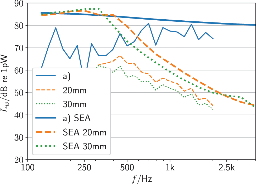
Figure 12.23 Radiated acoustic power of case 12.17a under force excitation. Source: Alexander Peiffer.
12.3.4 Full Scale SEA Models
The number of sources and excitation mechanisms in combination with the different drive conditions constitutes a vast amount of data that would be required to predict the interior noise level even when only airborne excitation is considered. Thus, in industrial applications, SEA models of cars are less applied for the prediction of noise levels and the achievement of specific target levels. Nevertheless, SEA is used early in the vehicle development program to evaluate the noise and vibration status of cars before a prototype has been built. For this purpose a full SEA model is required that includes all paths and sources of a car. Classical SEA models are introduced by Venor and Burghardt, Marc (2005) and Venor et al. (2003) and include many details as shown in Figure 12.24.

Figure 12.24 Full SEA model of a sedan car with combustion engine. Source: Alexander Peiffer.
According to the simulation strategy from Figure 12.15, most structural parts have to be modelled by FEM because they are still deterministic at 1000 Hz. The detailed substructuring shown in Figure 12.24 results from the restrictions of the 3D geometry modelling of the used software and leads to even smaller structural subsystems. Every cavity must be constituted by surrounding patches, and in most cases only edges can be connected. Due to this fact many subsystems have less than one mode in the third octave band. Thus, hybrid models would be excellent to fill this mid frequency gap as shown by Charpentier et al. (2008). However, the application of hybrid theory may suffer from the fact that FE and SEA methods are not yet practically implemented (Peiffer, 2016).
When Venor et al. (2003) developed the global simulation strategy, the hybrid theory was not available. Therefore, SEA was used for all components but enriched with many modifications to the coupling and damping loss factors so that the simulation results fits to the measurement results. It is especially due to this fact that SEA has the reputation of requiring a high level of experience.
12.3.4.1 Cavities
The first important step in the modelling strategy is a realistic representation of the exterior noise field and wave propagation around the car.
In Figure 12.25 the shape of the cavities and the sound field at 1000 Hz resulting from the rear tire rolling noise is shown, which follows from the adaption proposed by Venor. The outer cavities are connected to a small semi infinite fluid. The interior cavity subdivision follows from the given shape of most inner volumes, but the passenger cavity is further separated. The idea of this additional subdivision is to get different noise levels at different positions in the car, but it violates the week coupling requirement of SEA. This dilemma can also be solved by ray tracing or other gradient methods as shown by Schell and Cotoni (2015).

Figure 12.25 Exterior near, under floor, and far field cavities proposed by Venor et al. (2003) to represent sound field and propagation around the car. Source: Alexander Peiffer.

Figure 12.26 Subdivision of passenger cavity, engine bay, trunk, and many other hollow volumes. Source: Alexander Peiffer.
12.3.4.2 Carbody
The carbody structure (Figure 12.27) is modelled by several flat and curved plates that are in some cases quite small due to the given restrictions. Many parts in a car are treated with damping material so that the damping loss factors can be very high (). The error resulting from the small subsystems is therefore somehow limited; however, the subdivision of the carbody structure requires much experience to cope well with the realistic bending wave propagations along the carbody and over many subsystems.

Figure 12.27 Plate subsystem configuration of the SEA carbody model with force excitation at the front longeron with N. Source: Alexander Peiffer.
12.3.4.3 Noise Control
The noise control of cars is done by a diversity of foams, fibers, and damping and absorption material. Each lay-up is considered in detail and with varying thickness because of the beaded steel plates. Every single plate that is treated with such material is modelled with the transfer matrix method as introduced in section 10.5.2. In Figure 12.28 the variety of shell properties and noise control treatments are denoted.

Figure 12.28 Car plate subsystems with different colors for different property and noise control treatment. Source: Alexander Peiffer.
12.4 Trains
Vibroacoustic analysis of train structures in many ways resembles that of aircraft structures: the size is similar, and the structural lay-up and the materials applied display similarities (although the use of composites is pushed further for aircraft). Rail carbodies generally consist of a stiffened metal carbody structure, typically in steel or aluminum, with acoustically decoupled wall panels and walking floors making up the interior. All-in-all, the carbody constitutes a double wall structure with layers of thermal and acoustic insulation (fiberglass and foams) in the cavity. Recent body-shell concepts are based on GFRP or metal face sandwich. Like in aircraft, the walking floor structures are typically made using a sandwich material (honeycomb core or alike), but also wooden floors are common.
12.4.1 Structural Design
Steel carbodies are built in mild or stainless quality steels for which the sheeting is stiffened by beams in different layouts (Figure 12.29). For aluminum carbodies, wall, roof, and floors are normally made from extruded hollow profiles that are welded together (Figure 12.30). Aluminum carbodies can be made lighter than corresponding steel structures and can also be made to a high degree of pressure tightness, making them popular for high-speed trains. In addition, multi-material composite designs, often based on sandwich technologies, are increasingly being applied. These make use of the high stiffness properties of sandwich materials while providing smooth surfaces, beneficial for the interior assembly and exterior aesthetics. Furthermore, GFRP sandwich is the most common material for cab-structures due to its flexibility in shaping the exterior.

Figure 12.29 Structural layout of steel body-shell.
Reproduced with permission from (Orrenius et al., 2003).

Figure 12.30 Structural layout of extruded body-shell section.
Reproduced with permission from (Orrenius et al., 2003).
12.4.2 Interior Design
To minimise transfer of acoustical energy to the inner floor and lining panels, these are normally designed to be acoustically decoupled from the structure. Floating floor arrangements are applied, as illustrated in Figure 12.31. The system illustrated has rubber springs with a conical shape, designed for a controlled system resonance independent of load. The walking floor may also be continuously supported on a foam or fiber mat.

Figure 12.31 Floating floor arrangement.
Reproduced with permission from (Orrenius et al., 2003).
12.4.3 Excitation and Transmission Paths
Noise sources on a rail vehicle can be categorized into two groups: (i) those associated with rail–wheel interaction, namely radiation and vibrations from wheel and rail and sleepers (Thompson et al., 2009) and (ii) those of vehicle components (Bistagninio et al., 2015). The latter group can be divided into subgroups with (a) components for which fans and other cooling devices are the main source and (b) components with a vibrating shell being the main source, e.g. due to electromagnetic forces (transformers, motors) or mechanical contact (gear boxes). At very high speeds components with aerodynamic sources (c) become increasingly important, e.g. bogies and pantographs (Thompson et al., 2009).
The main sources of a rail car in operation are depicted in Figure 12.32. Please note that the relative importance of the sources are strongly speed dependent. For a train at standstill, several auxiliary systems contribute to the interior levels: HVAC, transformers, electric motor, and diesel engine cooling fans (Orrenius et al., 2007). During acceleration (and retardation), drive system noise from gears and motors is typically the main source for interior noise. Such noise is generally of a tonal character and can therefore be very annoying. The transmission to the interior is rather dominated by the structural forces than the sound levels generated in the bogie (although an accelerating motor can be very loud).

Figure 12.32 Vibroacoustic sources and transmission paths of rail car in operation.
Reproduced with permission from Ulf Orrenius.
At speeds above approximately 50 km/h, rolling noise typically becomes the main source. The excitation originates from imperfections on the rail head and wheels. For source modelling purposes these imperfections as well as the wheel and track properties must be described well (Thompson et al., 2009), which is typically handled within a dedicated software Twins (Jiang et al., 2011). For rail cars with under floor mounted diesel engines, structural vibration from the propulsion systems may exceed that of the rolling noise and is the main reason why electric trains provide a better acoustic comfort than diesel trains. Please note that for diesel engines, the main transmission path to the interior is typically via structural vibrations. At speeds above 250 km/h, low frequency aeroacoustic excitation becomes increasingly important. Such excitation is typically due to different objects interacting with the external flow, e.g. bogies, antennas, and the pantograph, rather than the TBL excitation as for a smooth aircraft fuselage. Note that locally, e.g. for passenger seats below the pantograph, aeroacoustic sources may dominate also at lower speeds.
12.4.4 Simulation Strategy
Being large enough to ensure sufficient modal densities and at a complexity level that both supports the use of a statistical model description and rather straightforward substructuring, train structures are generally suitable for SEA. From a passenger perspective the main sources are in the vicinity of the bogie. Therefore, vibroacoustic simulation models typically focus on the cross-section above the bogie. In addition, for high-speed trains, the driver’s cab as well as the pantograph cross-sections, are critical. For a carbody cross-section of, say, three meters length, the size of the structure in combination with the broad frequency excitation, makes standard FE models inappropriate for audio frequency interior noise predictions and must be combined with high frequency methods like SEA or ray tracing.

Figure 12.33 SEA model of a metro cross-section above the bogie from early transmission modelling work Stegemann (2002). Source: Alexander Peiffer.
The use of hybrid FEM/SEA models is helpful. Apart from being better suited for realistic excitation mechanisms, they offer a major improvement to standard SEA because of the possibility to simulate a structure containing both deterministic and statistical subsystems and thereby to cover a widened frequency range. In addition, including FEM subsystems much improves the chances to represent important excitation mechanisms, like aeroacoustics pressure fluctuations and structural forces from rolling sources and the traction system, with the accuracy needed for industrial predictions.
12.4.5 Applications to Rail Structures – Double Walls
The double wall model as outlined in Figure 12.34 is appropriate for most rail carbody structures. The model includes additional paths which describe the double leaf nonresonant system in addition to the mass law path, and is required to correctly represent the physics at and below the double wall resonance. The main double wall path T15 in Figure 12.34 corresponds exactly to equation (9.121). All other paths can be derived by modification of this formula. In case of low damping in the center cavity, the double wall junction must be used carefully, because it may lead to using the overall mass law path twice as shown by Wang (2015). However, real structures typically have lossy foams or fibers in the cavity, which simplifies the ananlysis.

Figure 12.34 Double wall SEA block diagram with additional paths for double leaf calculation. Source: Alexander Peiffer.
Complicating factors are modelling and quantification of the coupling mechanisms between inner and outer walls: elastic elements, air-spring, edge conditions, etc; and also to correctly account for the vibroacoustic properties of the carbody parts, typically manufactured in rib-stiffened corrugated steel sheets or assembled from so-called extruded panels. These topics are further discussed by, e.g. Craik (1996); Orrenius et al. (2005); Cherif et al. (2017).
12.4.5.1 Carbody Elements from Extruded Profiles
As explained above, most carbodies are made in either steel or aluminum. In the following we will focus on extruded aluminum structures as they are rather challenging to model. Due to their poor acoustic insulation properties, they are also subject to extensive noise control treatments. Steel carbody designs much resemble those of aircraft fuselage structures as discussed in section 12.2.
SEA models for structures made from extruded profiles should account for the fact that the vibrational modes relevant for sound radiation can be divided into two groups: global and local modes (Orrenius et al., 2005; Li et al., 2021). This also applies to many other stiffened engineering structures like those of aerospace and ships, but the cut-on frequencies for the local modes are typically relatively higher for rail structures.

Figure 12.35 Schematic of energy flow paths for a train floor assembled from extruded panels.
Reproduced with permission from Orrenius et al. (2005).
At low frequencies these profiles can be modelled by equivalent plate theory as their cross-sections do not deform when vibrating, see Figure 12.36a. At higher frequencies the individual subpanels start to vibrate independently, and the transmission is determined by the properties of these panels, see 12.36b. The frequency at which the subpanels start to have resonances is here referred to as the local cut-on frequency, typically at 400-500 Hz. Also important are the coincidence frequencies above which the structure radiates sound efficiently. For global modes, for which the panel structure vibrates as a whole, the coincidence frequency is typically between 130 and 170 Hz, while for the subpanel modes coincidence occurs around 4 kHz. The combined width of the two coincidence regions is one reason for poor sound reduction properties. See reference (Pang, 2004; Li et al., 2021) for examples of measured and calculated radiation efficiencies.

Figure 12.36 Example of local and global cross section modes determined from wave-guide finite elements.
Reproduced with permission from Orrenius et al. (2005).
Resulting transmission losses for low and high frequency models are displayed in Figure 12.37, highlighting the need for including both modal groups as parallel sub-systems in a model. The benefit of separating global and local modes is also clear when examining calculated insertion loss of damping layers, as shown in Figure 12.38. Damping applied on the upper surface of the panel is mainly effective above the cut-on frequency of the local modes. Also, calculated panel radiation efficiencies and velocity level differences are useful indicators of model validity, see Orrenius et al. (2005) and Li et al. (2021) for comparasions of measured and caculated data.

Figure 12.37 TL of Metro floor with added damping layer (Pang, 2004). Source: Alexander Peiffer.

Figure 12.38 Insertion loss from application of damping layer measured and calculated (Orrenius et al., 2005). Source: Alexander Peiffer.
Alternatively, periodic cell theory can be applied to derive an SEA model from a small structural FE model with periodical boundary conditions (Cotoni et al., 2008). Such procedures are successfully applied for extruded profiles by Orrenius et al. (2009a) and for aluminum aircraft structures (Orrenius et al., 2009b). In Wittsten (2016) the concept is applied to minimize the weight of an extruded train floor, subject to acoustical and structural constraints.

Figure 12.39 Schematic of floating floor arrangements with the walking floor resting on rubber mount. The air cavity is filled with foam material.
Reproduced with permission from Ulf Orrenius.
The periodic cell concept was also applied in work presented in (Orrenius et al., 2014) in which a complete floor assembly as depicted in Figure 12.40 was analyzed. Airborne transmission via the cavity is not included in the FE model and was added separately from using a standard double wall SEA model but with the springs disconnected, and the total transmission coefficient is determined as where the airborne and structure borne transmission are denoted and , respectively. For the transmission through the extruded panel, the fluid structure coupling was determined by input data from running the periodic cell model without the top floor. The Metawell inner floor was modelled as a sandwich panel with equivalent core, and the rubber spring elements were modelled as lossy linear springs.

Figure 12.40 Left: Periodical cell model of the train floor. Right: Structural and airborne transmission. Source: Alexander Peiffer.
In Figure 12.41 the total transmission loss calculated is plotted together with the airborne and structure borne paths indicated. The airborne path dominates at low frequencies whereas the structural path dominates at high frequencies. Also, the measured transmission loss is displayed. The match between measured and calculated results is reasonable throughout the frequency range, although the SEA double wall model grossly underestimates the low frequency TL. Please note that the double wall junction functionality applied here accounts for indirect coupling between the sending and receiving cavity as well as between sending cavity and receiving panel and vice versa, see Figure 12.34.

Figure 12.41 Structural vs. airborne transmission loss: Calculated and measured results. Source: Alexander Peiffer.
For the assembly analyzed, the direct coupling between the two panels via connecting joints and constrained air was so strong that it dominates the transmission into the receiving panel. This suggests that additional absorption in the center cavity, e.g. by means of absorption material, or damping material applied on the extruded panel will not increase the transmission loss much unless this transmission is significantly reduced. The model thus provides a physical explanation to discouraging results from measurements on such noise control treatments. Instead, for increased sound and vibration insulation, the direct coupling between the panels should preferably be relaxed, e.g. by increasing the distance between the walls, or using softer rubber elements. Typically, the spring elements are mounted on top of the web intersections of the extruded panels, the location with highest input impedance, position A in Figure 12.42. However, for practical reasons, such mounting is not always possible. A parameter study was undertaken, in which the spring elements were offset from the web intersection of the extruded panel by 20% and 50% of the division between the webs.

Figure 12.42 Cross-section of FE model with location of spring elements indicated: A, nominal; B, 20% offset; C, 50% offset. Source: Alexander Peiffer.
Transmission loss with different element locations is shown in Figure 12.43. It is notable that already 20% offset significantly reduces the transmission loss. One reason is that with offset springs, the lossy rubber elements are less deflected, and the modal loss factors of the inner floor modes are significantly reduced.

Figure 12.43 Transmission loss with different spring element locations. Source: Alexander Peiffer.
12.4.6 Carbody Sections – High Speed Applications
At higher speeds the source ranking drastically changes with the onset of aeroacoustic sources. For exterior noise, aeroacoustics becomes significant above speeds of 300–320 km/h. As the speed dependence is typically , rather than as for the rolling sources (Thompson et al., 2009), they become dominant at higher speeds. For interior noise, aeroacoustics may locally be significant also at lower speeds, e.g for driver’s cabs and for areas below the pantograph.
12.4.6.1 Roof Structures
Train roof structures are critical at high speeds when high noise and vibration levels are generated from pantographs and antennas etc. In Figure 12.44 an FEM/SEA model of a roof structure is depicted (Orrenius and Kunkell, 2011). The lower SEA cavity represents the passenger compartment, coupled to the inner ceiling and walls. The upper cavity represents the outside and was coupled to the roof. Generally, the aluminum roof structure was modelled in FE whereas the interiors, including the fluid cavities, were modelled using SEA subsystems. The ceiling was made from a sandwich with 12 mm plywood core covered with 1 mm aluminum face panels. However, the core was not homogeneous but contained a grid of rectangular m2 cut-outs, where the ceiling essentially consisted of an aluminum double shell, see (Orrenius and Kunkell, 2011)). As the first resonance frequency of the AAA-panels in the cut-outs is quite low, 45 Hz assuming simply supported boundaries, it was decided to model all cut-outs with one single SEA system and the rest of the sandwich with another SEA subsystem. The constrained air in the cut-out cavity was modelled as a linear spring. In addition, SEA subsystems representing the ventilation airducts were added. Thus, in the model, three parallel SEA systems were connecting the compartment cavity to the roof cavity above the ceiling (not shown in the figure).

Figure 12.44 FEM/SEA model of a train roof structure. The duct cavities and the roof spacing cavity are hidden. “AAA” is aluminum–air–aluminum sandwich, and “APA” is aluminum–plywood–aluminum sandwich.
Reproduced with permission from Orrenius and Kunkell (2011).
In Figure 12.45 calculated input powers via different paths into the roof cavity are displayed. Missing data are due to too few modes in the band. The aluminum–air–aluminum sandwich path dominates the transmission. The calculated transmission loss is shown to match that measured according to ISO 15186-2 by scanning of the outer roof with an intensity probe while exciting the interior using an omnidirectional loudspeaker. The model has been used for parametric studies to assess the effect of noise control treatment applied on the ceiling structure (Orrenius and Kunkell, 2011).

Figure 12.45 Input powers to roof cavity (Orrenius and Kunkell, 2011). Source: Alexander Peiffer.

Figure 12.46 Measured and simulated transmission loss of roof (Orrenius and Kunkell, 2011). Source: Alexander Peiffer.
The pantograph becomes a very important source at high speeds and in this section, results from a pantograph noise transmission study are presented. The pantograph analyzed is mounted on vibration isolators at three connection points in a roof recess; see Figures 12.32 and 12.47. Due to the aerodynamic forces and the contact with the electrical overhead line, vibrations are generated and transmitted via point forces on the roof. In the study presented, forces from wind tunnel measurements were applied (Brick et al., 2011) with operational pantograph (not folded) but without the influence of the overhead lines.

Figure 12.47 Left: Aeroacoustic simulation of pantograph in recess. (Right) FEM/SEA model of pantograph recess with CFD determined pressure field and structural forces.
Reproduced with permission from (Orrenius and Kunkell, 2011).
A hybrid FEM/SEA model was created for the high-speed train roof. A computational fluid dynamics (CFD) model was used to determine the pressure fluctuations in the recess. In Figure 12.47 the model is displayed with the positions of the pantograph loads indicated as well as the CFD mesh. The CFD pressure field spectra were then projected onto the modal basis, representing the FE part of the roof structure. For this construction the design of the interior ceiling is made in a flat thin GRP panel, thus more suitable to SEA than the ceiling described above. The roof spacing cavity is filled with an absorbing material, here modelled according to Delany and Bazley (1970) with the material described simply by its flow resistivity and density. Figure 12.48 shows the power input into the compartment for the three types of excitations: the pantograph structural forces, the pressure field in the recess, and (for reference) a turbulent boundary layer applied to the entire carbody circumference.

Figure 12.48 Power input to compartment at 350 km/h (Orrenius and Kunkell, 2011). Source: Alexander Peiffer.
Combination of experimental data for the dynamic forces on the pantograph feet with pressure data from compressible and nonstationary CFD is a practical approach that serves its purpose well in view of the difficulty in predicting the dynamic forces. The calculations were carried out at a speed of 350 km/h whereas the windtunnel measurements were made at 280 km/h. Accordingly, the dynamic forces were scaled according to the speed dependence determined at the measurements (Orrenius and Kunkell, 2011).
The CFD pressure data available were determined for the recess only without the pantograph. To determine the effect of the uplifted pantograph, a correction term was applied based on measured wall pressure difference in the cavity with and without the uplifted pantograph. However, the spectral details were not considered for this correction which underestimates, e.g. the tonality associated with Strouhal effects. Alternatively, CFD calculations with the uplifted pantograph could have been used. In this case the pressure field would need to be complemented by the acoustic excitation of the pantograph, e.g. by using Lighthill’s analogy (Lighthill, 1953).
A benefit of a coupled FEM/SEA model in this context is that parametric studies of the ceiling design including noise control treatments can readily be made without updating the FE model. Transmission path analysis is also straightforward.
12.4.6.2 Cab Structures
For cab structures, modal models based on FE can be solved up to a few kHz but need to be combined with either ray tracing or SEA for the interior cavity (Kirchner et al., 2012). Also the cab interior trim panels in, eg, honeycomb, plastic, or foam-covered sheet metal, are typically suitable for SEA modelling (or TMM). A Hybrid FEM/SEA approach is useful to analyze aeroacoustics noise with dominating power below 1 kHz, for which the receiving structures, like the floor above the bogie and the wind screen, are modelled with FE. Also, structural sources like vibrations transferred via bogie coupling elements, can be analyzed in this way. Like for the pantograph example above, vibration velocities measured at the mounting point of the coupling elements can be used together with FE calculated impedances to determine input powers. In Figure 12.49 two FEM/SEA models are displayed for low and high frequency analysis of a high-speed train cab. The low frequency model ( kHz) contains mainly FE subsystems (335 000 elements), with interior panels and air cavities modelled with SEA subsystems. The floor pressure load is taken from CFD calculations and the structural forces on the yaw damper mounting point from in-situ testing. The high frequency model ( kHz) is mainly made up of SEA subsystems, with only the windscreen modelled in FE. In this particular case the airborne transmission through the floor was taken from test data.

Figure 12.49 Left: Low frequency hybrid FEM/SEA model of cab structure with the pressure load determined from CFD. Right: High frequency model for wind screen aeroacoustic analysis.
Reproduced with permission ALSTOM Holdings SA, 46 rue Albert Dhalenne 93000 St Ouen-sur-Seine, France. Alstom Group is the owner of all copyrights on these images herebefore listed.
In 12.50, calculated cab sound levels are displayed together with data measured from a different high-speed cab at the same speed. Transfer path analysis was made to reveal the major transmission paths, which is highly useful in the design process when assessing the effect of various control measures. In this case it was shown that an increase in speed will mainly increase the low frequency transmission from the bogie area (aeroacoustics).

Figure 12.50 Calculated and measured sound levels in the cab cavity at 320 km/h. The measurements are from a different train but at the same speed.
Reproduced with permission ALSTOM Holdings SA, 46 rue Albert Dhalenne 93000 St Ouen-sur-Seine, France. Alstom Group is the owner of all copyrights on these images herebefore listed.
12.5 Summary
The aim of the presented test cases is to highlight different aspects and issues of vibroacoustic simulation. In the industrial context the task of simulation is mostly to support the design process in the early development phase but also to find the best solutions in later project phases. This later period is sometimes a ’fire fighting’ phase but even then the simulation can support the test and the development of countermeasures for a specific acoustic problem. However, the creation of a precise simulation model is a demanding task that requires experience and knowledge of the simulation method. The experience is mandatory because we need a feeling for the correct subsystem description and the level of abstraction that is reasonable. It hopefully became clear, that the model generation and application is far from being done based on simple recipes.
Bibliography
- Jean-F. Allard and Noureddine Atalla. Propagation of Sound in Porous Media. Wiley, second edition, 2009.
- W.V. Bhat. Flight test measurement of exterior turbulent boundary layer pressure fluctuations on Boeing model 737 airplane. Journal of Sound and Vibration, 14(4): 439–457, February 1971. .
- M. A. Biot. Generalized Theory of Acoustic Propagation in Porous Dissipative Media. The Journal of the Acoustical Society of America, 34(9A): 1254–1264, September 1962.
- A. Bistagninio, G. Squicciarini, Ulf Orrenius, E. Bongini, M. Starnberg, R. Cordero, J. Sapena, and D. J. Thompson. Acoustical Source Modelling for Rolling Stock Vehicles: The Modeller’s Point of View, Proceedings Euronoise 2015,. In Euronoise, pages 1991–1996, 2015.
- Michael Blundell and Damian Harty. Multibody Systems Approach to Vehicle Dynamics. Automotive Engineering. Elsevier Butterworth-Heinemann, Amsterdam Heidelberg, transferred to digital print edition, 2010.
- M. Bouhaj, O. von Estorff, and A. Peiffer. An approach for the assessment of the statistical aspects of the SEA coupling loss factors and the vibrational energy transmission in complex aircraft structures: Experimental investigation and methods benchmark. Journal of Sound and Vibration, 403: 152–172, September 2017. .
- Heike Brick, Torsten Kohrs, Ennes Sarradj, and Geyer. Noise from high-speed trains: Experimental determination of the noise radiation of the Pantograph. In Proceedings Forum Acousticum, Aalborg, Denmark, July 2011.
- Arnaud Charpentier, Prasanth Sreedhar, Julio Cordioli, and Kazuki Fukui. Modeling process and validation of Hybrid FE-SEA method to structure-borne noise paths in a trimmed automotive vehicle. In Proceedings 2008 SAE BRASIL Noise and Vibration Conference, March 2008.
- Raef Cherif, Andrew Wareing, and Noureddine Atalla. Evaluation of a hybrid TMM-SEA method for prediction of sound transmission loss through mechanically coupled aircraft double-walls. Applied Acoustics, 117: 132–140, February 2017.
- J.A. Cockburn and J.E. Robertson. Vibration response of spacecraft shrouds to in-flight fluctuating pressures. Journal of Sound and Vibration, 33(4): 399–425, April 1974.
- G. M. Corcos. Resolution of Pressure in Turbulence. The Journal of the Acoustical Society of America, 35(2): 192–199, 1963.
- V. Cotoni, R.S. Langley, and P.J. Shorter. A statistical energy analysis subsystem formulation using finite element and periodic structure theory. Journal of Sound and Vibration, 318(4-5): 1077–1108, December 2008. .
- Vincent Cotoni, Robin Langley, and Phil Shorter. A Statistical Energy Analysis Subsystem Formulation using Finite Element and Periodic Structure Theory. In Proceedings NOVEM 2009, page 12, Oxford, England, April 2009.
- Robert J M Craik. SEA for buildings. Noise and Vibration Worldwide, 27(6):13–, June 1996.
- Peter Davidsson. Structure-Acoustic Analysis; Finite Element Modelling and Reduction Methods. PhD other, Lund University, Lund, Sweden, August 2004.
- Evan B. Davis. By Air by SEA. In Noise-Con 2004, pages 12–17, Baltimore, Maryland, July 2004.
- Carlos de Matos. Simulation des Schalldurchgangs einer Flugzeugwand. Diploma other, TU-Hamburg Harburg, Hamburg, Germany, February 2008.
- ME Delany and EN Bazley. Acoustical properties of fibrous absorbent materials. Applied acoustics, 3(2): 105–116, 1970.
- B.M. Efimtsov and L.A. Lazarev. Forced vibrations of plates and cylindrical shells with regular orthogonal system of stiffeners. Journal of Sound and Vibration, 327(1–2):41–54, October 2009.
- Javier García de Jalón and Eduardo Bayo. Kinematic and Dynamic Simulation of Multibody Systems The Real-Time Challenge. 1994.
- Klaus Genuit, editor. Sound-Engineering im Automobilbereich: Methoden zur Messung und Auswertung von Geräuschen und Schwingungen. Springer, Heidelberg, 2010.
- Michael Goody. Empirical Spectral Model of Surface Pressure Fluctuations. AIAA Journal, 42(9): 1788–1794, September 2004.
- Shijie Jiang, P. Meehan, David Thompson, and C Jones. Railway rolling noise prediction under European conditions. Australian Acoustical SocietyConference 2011, Acoustics 2011: Breaking New Ground, page 8, January 2011.
- Karl-Richard Kirchner, F. Brännström, Ulf Orrenius, and R. Hallez. aeroacoustic noise generation and transmission modelling for a high-speed train driver’s cab. In Proceedings Internoise 2012, New York, USA, 2012.
- Alexander Klabes, Christina Appel, Michaela Herr, and Sören Callsen. Fuselage Excitation During Cruise Flight Conditions: A New CFD Based Pressure Point Spectra Model. In Proceedings, page 12, Hamburg, Germany, August 2016.
- L. Leylekian, M. Lebrun, and P. Lempereur. An Overview of Aircraft Noise Reduction Technologies. Aerospace Lab, (7): 15, June 2014.
- Hui Li, Giacomo Squicciarini, David Thompson, Jungsoo Ryue, Xinbiao Xiao, Dan Yao, and Junlin Chen. A modelling approach for noise transmission through extruded panels in railway vehicles. Journal of Sound and Vibration, 502: 116095, June 2021. .
- M.J. Lighthill. On sound generated aerodynamically I. General theory. Proceedings of the Royal Society A: Mathematical, Physical and Engineering Science, 221: 24, 1953.
- B.R. Mace and P.J. Shorter. Energy flow models from finite element analysis. Journal of Sound and Vibration, 233(3): 369–389, June 2000.
- Gideon Maidanik. Response of Ribbed Panels to Reverberant Acoustic Fields. The Journal of the Acoustical Society of America, 34(6): 809–826, June 1962.
- Laurent Maxit, Marion Berton, Christian Audoly, and Daniel Juvé. Discussion About Different Methods for Introducing the Turbulent Boundary Layer Excitation in Vibroacoustic Models. In Elena Ciappi, Sergio De Rosa, Francesco Franco, Jean-Louis Guyader, and Stephen A. Hambric, editors, Flinovia - Flow Induced Noise and Vibration Issues and Aspects, pages 249–278. Springer International Publishing, Cham, 2015.
- Vinod G. Mengle, Ulrich W. Ganz, Eric Nesbitt, Eric J. Bultemeier, and Russell H. Thomas. Flight Test Results for Uniquely Tailored Propulsion-Airframe Aeroacoustic Chevrons: Shockcell Noise. In Proceedings, volume 2439, page 17. American Institute of Aeronautics and Astronautics(AIAA), 2006.
- U. Orrenius, V. Cotoni, and A. Wareing. Analysis of sound transmission through periodic structures typical for railway car bodies and aircraft fuselages. INTER-NOISE and NOISE-CON Congress and Conference Proceedings, 2009(8): 785–796, 2009a.
- Ulf Orrenius and H. Kunkell. Sound Transmission through a High-Speed Train Roof. In Proceedings ICSV 2011, Rio, Brasil, 2011.
- Ulf Orrenius, E. Lundberg, and Bert Stegemann. Noise Control Elements in Train Design: An Overview of Solutions for Carbody Floors. In Proceedings ICSV 2013, Stockholm, Sweden, 2003.
- Ulf Orrenius, Y.Y. Pang, and Bert Stegemann. Acoustic modelling of extruded profiles for railway cars. In Proceedings NOVEM 2005, St. Raphael, France, 2005.
- Ulf Orrenius, Siv Leth, and Anders Frid. Noise reduction at urban hot-spots by vehicle noise control. In Proceedings IWRN 2007, München, Germany, 2007.
- Ulf Orrenius, A. Waering, and Vincent Cotoni. Analysis of sound transmission through aircraft fuselages excited by turbulent boundary layer or diffuse acoustic pressure fields. In Proceedings NOVEM 2009, Oxford, England, 2009b.
- Ulf Orrenius, Hao Liu, Andrew Wareing, Svante Finnveden, and Vincent Cotoni. Wave modelling in predictive vibro-acoustics: Applications to rail vehicles and aircraft. Wave Motion, 51(4): 635–649, June 2014.
- Dan Palumbo. Determining correlation and coherence lengths in turbulent boundary layer flight data. Journal of Sound and Vibration, 331(16): 3721–3737, April 2012.
- Y.Y. Pang. Modelling acoustic properties of truss-like periodic panels: Application to extruded aluminium profiles for railway structures. Master’s other, KTH Stockholm, Stockholm, Sweden, 2004.
- Alexander Peiffer. Comparison of the computational expense of hybrid FEM/SEA calculation. In Proceedings NOVEM 2012, Sorrento, Italy, April 2012.
- Alexander Peiffer. Full frequency vibro-acoustic simulation in the aeronautics industry. In Proceedings, Leuven, Belgium, September 2016.
- Alexander Peiffer and Uwe Christian Mueller. Review of Efficient Methods for the Computation of Transmission Loss of Plates with Inhomogeneous Material Properties and Curvature Under Turbulent Boundary Layer Excitation. In Elena Ciappi, Sergio De Rosa, Francesco Franco, Jean-Louis Guyader, Stephen A. Hambric, Randolph Chi Kin Leung, and Amanda D. Hanford, editors, Flinovia–Flow Induced Noise and Vibration Issues and Aspects - II, pages 233–251. Springer International Publishing, Cham, 2019.
- Alexander Peiffer and Zhiyi Wang. SEA Simulation einer Flugzeugseitenwand und Korrelation zu Testdaten. In Fortschritte der Akustik, page 4, Nürnberg, Germany, April 2015.
- Alexander Peiffer, Stephan Brühl, and Daniel Redmann. Hybrid Modelleing of Random Excitation of Shell Structures. In Proceedings NOVEM 2009, Oxford, England, April 2009.
- Alexander Peiffer, Mahjoub Mezni, and Clemens Moeser. Hybrid Modelling of Deterministically Loaded Subsystems. In Proceedings 18th International Congress on Sound and Vibration, page 8, Rio, Brasil, July 2011.
- Alexander Peiffer, Clemens Moeser, and Arno Röder. Transmission loss modelling of double wall structures using hybrid simulation. In Fortschritte Der Akustik, pages 1161–1162, Merano, March 2013.
- Alexander Peiffer, Clemens Moeser, Koen De Langhe, and Robin Boeykens. SIMULATING SOUND TRANSMISSION LOSS THROUGH AIRCRAFT FUSELAGE PANELS: AN UPDATE ON RECENT TECHNOLOGY EVOLUTIONS. In Proceedings of NAFEMS 2015, page 20, San Diego, June 2015.
- Alexander Schell and Vincent Cotoni. Prediction of Interior Noise in a Sedan Due to Exterior Flow. SAE International Journal of Passenger Cars - Mechanical Systems, 8(3): 1090–1096, June 2015.
- Bert Stegemann. Development and validation of a vibroacoustic model of a metro rail car using Statistical Energy Analysis (SEA). Master’s other, TU-Berlin, Berlin, 2002.
- Stephan Tewes and Alexander Peiffer. Abschlussbericht RAST. Technical Report BMBF-FKZ-03CL09A-Abschlussbericht-RAST, EADS IW SP-NV, Hamburg, Germany, December 2013.
- D. J. Thompson, Chris Jones, and Pierre-Etienne Gautier. Railway Noise and Vibration: Mechanisms, Modelling and Means of Control. Elsevier, Amsterdam; Boston, 1st ed edition, 2009.
- Joe Venor and Burghardt, Marc. SEA MODELLING AND VALIDATION OF SOUND-FIELDS AND SEALS IN AUTOMOBILES. In Conference Proceedings, page 7, Potsdam, Germany, 2005.
- Joe Venor, A. Müller, and Silje Nintzel. SEA MODELLING AND VALIDATION OF STRUCTURE AND AIRBORNE INTERIOR NOISE IN AN AUTOMOBILE. In Proceedings Vibro-Acoustic Users Conference Europe, page 8, Leuven, Belgium, January 2003.
- Xu Wang, editor. Vehicle Noise and Vibration Refinement. Woodhead Publishing in Mechanical Engineering. CRC Press, Boca Raton, 2010.
- Zhiyi Wang. Correlation between SEA Simulation and Test Results for a Double Wall Structure. Master’s other, TU-München, München, Germany, June 2015.
- Christian Weineisen. Modellierung einer Flugzeugstruktur mit der Statistischen-Energieanalyse. Master’s other, Technische Universität München(TUM), München, Germany, March 2014.
- J. Wittsten. Optimization of Train Floors with Acoustic and Structural Constraints. Master’s other, Chalmers University of Technology, Chalmers, Sweden, 2016.
- Peter Zeller, editor. Handbuch Fahrzeugakustik: Grundlagen, Auslegung, Berechnung, Versuch; mit 43 Tabellen. ATZ/MTZ-Fachbuch. Vieweg + Teubner, Wiesbaden, 1. aufl edition, 2009.
Notes
- 1 [email protected]
- 2 In 18 years of work at Airbus, I didn’t find someone who could explain to me the acronym DADO. In English literature some authors call them catwalk panels.