11
Hybrid Systems

Basically, we have already applied the hybrid theory in preceding sections, for example Section 7.4. In many cases there were deterministic systems in the junction, for example a plate that we have considered as deterministic connection between the two cavity SEA systems and using the deterministic transfer matrix of the plate.

The twin chamber is an excellent test case for the hybrid method, as it constitutes a clear separation between random and deterministic subsystems and provides all the details of how to deal with each single step of hybrid FEM/SEA simulation.

11.1 Hybrid SEA Matrix

For pure SEA models the matrix from equation (6.113) is applied. The hybrid SEA matrix is similar except one additional damping contribution caused by the damping from the connected FEM-subsystems.

StartLayout 1st Row with Label Start 1 By 1 Matrix 1st Row upper L Superscript prime Baseline EndMatrix equals Start 4 By 4 Matrix 1st Row 1st Column n 1 left-parenthesis eta 11 Superscript alpha Baseline plus sigma-summation Underscript n equals 1 Overscript upper N Endscripts eta Subscript 1 n Baseline right-parenthesis 2nd Column minus n 2 eta 21 3rd Column midline-horizontal-ellipsis 4th Column minus n Subscript upper N Baseline eta Subscript upper N Baseline 1 Baseline 2nd Row 1st Column minus n 1 eta 12 2nd Column n 2 left-parenthesis eta 22 Superscript alpha Baseline plus sigma-summation Underscript n equals 1 Overscript upper N Endscripts eta Subscript 2 n Baseline right-parenthesis 3rd Column Blank 4th Column vertical-ellipsis 3rd Row 1st Column vertical-ellipsis 2nd Column Blank 3rd Column down-right-diagonal-ellipsis 4th Column Blank 4th Row 1st Column minus n 1 eta Subscript 1 upper N Baseline 2nd Column midline-horizontal-ellipsis 3rd Column Blank 4th Column n Subscript upper N Baseline left-parenthesis eta Subscript upper N upper N Superscript alpha Baseline plus sigma-summation Underscript n equals 1 Overscript upper N Endscripts eta Subscript upper N n Baseline right-parenthesis EndMatrix EndLabel Blank EndLayout  (7.35)

All other impacts of the FE parts of the hybrid model are hidden in the hybrid coupling loss factors or an additional power input that may come from radiation of FE-subsystems into the SEA-subsystems.

11.2 Twin Chamber

Figure 11.1Twin chamber arrangement for TL tests of panel.
Source: Alexander Peiffer.

The twin chamber set-up is such a perfect example for the hybrid method, because both chambers are designed to be random by the large size and irregular shape. So, the two cavities can be considered as random subsystems for the complete frequency range. The panel that should be tested is supposed to be smaller than the panel from section 10.2.1. In this case it is not random and must be treated as a deterministic subsystem. We use the analytical solution of rectangular plate normal modes in the discrete version (5.41). As described in section 1.4.4.1 the normal modes are given as vectors and assembled in a matrix

Start 1 By 1 Matrix 1st Row normal upper Phi EndMatrix equals Start 1 By 4 Matrix 1st Row 1st Column Start 1 By 1 Matrix 1st Row normal upper Phi EndMatrix Subscript 1 Baseline 2nd Column Start 1 By 1 Matrix 1st Row normal upper Phi EndMatrix Subscript 1 Baseline 3rd Column midline-horizontal-ellipsis 4th Column Start 1 By 1 Matrix 1st Row normal upper Phi EndMatrix Subscript upper N EndMatrix

and the deterministic equations of motion are transformed into diagonal form. For the flat plate we use the mode shapes from equation (5.46) so that we can write the deterministic dynamic stiffness matrix in the following form

StartLayout 1st Row 1st Column Start 1 By 1 Matrix 1st Row bold-italic upper D prime Subscript s EndMatrix 2nd Column equals Start 1 By 1 Matrix 1st Row normal upper Phi EndMatrix Superscript upper H Baseline Start 1 By 1 Matrix 1st Row bold-italic upper D Subscript s Baseline EndMatrix Start 1 By 1 Matrix 1st Row normal upper Phi EndMatrix equals Start 4 By 4 Matrix 1st Row 1st Column omega 1 squared left-parenthesis 1 plus j eta right-parenthesis minus omega squared 2nd Column Blank 3rd Column Blank 4th Column Blank 2nd Row 1st Column Blank 2nd Column down-right-diagonal-ellipsis 3rd Column Blank 4th Column Blank 3rd Row 1st Column Blank 2nd Column Blank 3rd Column omega Subscript n Superscript 2 Baseline left-parenthesis 1 plus j eta right-parenthesis minus omega squared 4th Column Blank 4th Row 1st Column Blank 2nd Column Blank 3rd Column Blank 4th Column omega Subscript upper N Superscript 2 Baseline left-parenthesis 1 plus j eta right-parenthesis minus omega squared EndMatrix EndLayout  (11.1)

The radiation stiffness is calculated using (8.42) and also transformed into the modal space by

StartLayout 1st Row 1st Column Start 1 By 1 Matrix 1st Row bold-italic upper D Subscript dir Superscript prime left-parenthesis m right-parenthesis EndMatrix 2nd Column equals Start 1 By 1 Matrix 1st Row normal upper Phi EndMatrix Superscript upper H Baseline Start 1 By 1 Matrix 1st Row bold-italic upper D Subscript dir Superscript left-parenthesis m right-parenthesis Baseline EndMatrix Start 1 By 1 Matrix 1st Row normal upper Phi EndMatrix EndLayout  (11.2)

The global form of the coupling loss factor and the transmission coefficient remains unchanged

StartLayout 1st Row with Label eta Subscript m n EndLabel 1st Column equals StartFraction 2 Over pi n Subscript m Baseline omega EndFraction sigma-summation Underscript i comma j Endscripts upper I m left-brace bold-italic upper D Subscript dir comma i j Superscript prime left-parenthesis n right-parenthesis Baseline right-brace left-parenthesis Start 1 By 1 Matrix 1st Row bold-italic upper D Subscript t o t Baseline EndMatrix Superscript prime negative 1 Baseline upper I m Start 1 By 1 Matrix 1st Row bold-italic upper D Subscript dir Superscript left-parenthesis m right-parenthesis Baseline EndMatrix prime Start 1 By 1 Matrix 1st Row bold-italic upper D Subscript t o t Baseline EndMatrix Superscript prime negative upper H Baseline right-parenthesis Subscript i j Baseline 2nd Row 1st Column tau Subscript m n 2nd Column equals StartFraction 8 pi squared omega n Subscript m Baseline Over k Subscript m Superscript 2 Baseline upper A EndFraction eta Subscript m n Baseline upper T upper L equals 10 log Subscript 10 Baseline StartFraction 1 Over tau EndFraction EndLayout  (7.50)

The modal total stiffness matrix

Start 1 By 1 Matrix 1st Row bold-italic upper D Subscript t o t Superscript prime Baseline EndMatrix equals Start 1 By 1 Matrix 1st Row bold-italic upper D Subscript s Superscript prime Baseline EndMatrix plus sigma-summation Underscript m Endscripts Start 1 By 1 Matrix 1st Row bold-italic upper D Subscript dir Superscript prime left-parenthesis m right-parenthesis EndMatrix  (11.3)

requires some comment. The modal form of the direct radiation stiffness is a fully populated but symmetric matrix. Thus, the hybrid method destroys the diagonal form of the dynamic stiffness matrix. Though the introduction of random systems reduces the degrees of freedom tremendously, the computational amount can be higher than for a full deterministic method if the connecting regions are too large. See Peiffer (2012) for details. In Figure 11.2 the subsystem configuration is shown. We chose a rather small flat aluminium plate of size Lx=0.5 m and Ly=0.8 m of 4 mm thickness. At this size we will have a deterministic behaviour until 2 kHz.

Figure 11.2 System and loads setup for the hybrid twin chamber model.
Source: Alexander Peiffer.

The damping in the SEA systems due to the connected FE subsystems is given by (7.52)

eta subscript m m end subscript superscript alpha equals fraction numerator 2 over denominator pi omega n subscript m open parentheses omega close parentheses end fraction sum for i of eta omega subscript i superscript 2 open parentheses open square brackets bold italic D subscript bold t bold o bold t end subscript close square brackets to the power of italic apostrophe italic minus italic 1 end exponent I m open square brackets bold italic D subscript bold d bold i bold r end subscript superscript begin bold style stretchy left parenthesis m stretchy right parenthesis end style end superscript close square brackets to the power of italic apostrophe open square brackets bold italic D subscript bold t bold o bold t end subscript close square brackets to the power of italic apostrophe italic minus H end exponent close parentheses subscript i i end subscript  (7.52)

This damping loss corresponds to the dissipation in the cavities because of energy dissipated in the connected FEM plate. In comparison with the situation when the plate is an SEA subsystem, this part replaces the dissipation in the reverberant field of the plate.

For the execution of the full hybrid simulation process, we apply a random power load to the first SEA cavity and a deterministic out-of-plane point force at the plate near the corner. This creates the typical setup where we need both the random modelling of the reverberant fields in the cavity and the deterministic model of the plate. The random point force (3.230) will not provide a good estimation of the real input power, because the plate is a deterministic subsystem. Thus, the modal frequency response to this force excitation must be used. To summarize, two load cases are simulated:

Power 1W Power source in cavity 1

Force 10 N rms Point force on plate.

The global set-up of cavities is the same as in Chapter 10. The plate shall be deterministic for a large frequency range. In order to cover the coincidence region, we aim at calculating the frequency response up to f=4000 Hz. The hybrid modelling example is also useful for further clarification when and under which conditions the SEA assumptions become valid. Thus, all results will be compared to the results of an SEA model with the same data.

11.2.1 Step 1 – Setting up System Configurations

The normal modes of the plate are taken from equation 5.46. The modes are sorted in frequency order. The first mode shape with n=(1,1) is at f1=54.2 Hz; until fmax=4780.1 Hz there are 140 modes. The SEA properties of the cavities are taken from Chapter 10.

The direct field radiation stiffness matrices are calculated using a mesh of Nx=40 and Ny=25 nodes. This leads to a mesh of element length ΔxΔy0.02 m, which is sufficient for this frequency. When the structural plate modes shall be calculated using a FE-mesh, this must be fine enough for the bending wavelength and can thus be much finer than the mesh that is required for a precise radiation stiffness calculation in the desired frequency range. However, in this example it is not necessary, because we map the solution onto our mesh directly from analytical results.

When using fine FE meshes for the structure, it is better to use two meshes, each appropriate for structure and fluid, for the better use of (8.42).

11.2.2 Step 2 – Setting up System Matrices and Coupling Loss Factors

The total system matrix is created according to (11.3). All degrees of freedom are shared by the connected systems and no specific treatment of connecting region is required.

The SEA matrix is set up with the same principles as in section 7.3.2.1 and using equation (7.50). In the SEA matrix the plate does not occur as subsystem. Hence, for the energy degrees of freedom, we have a two system SEA matrix.

The result for the hybrid transmission loss of the plate is shown in Figure 11.3. In addition the SEA transmission loss is also included. We recognize the typical shape of the transmission loss as described, for example, in Bies et al. (2018). At low frequencies below the first resonances, the transmission is stiffness controlled and very high. The transmission loss drops down at the first panel resonances, increases, and reaches mass law slope above 500 Hz. At this frequency the wavelength in the fluid becomes similar to the panel dimensions. There is a good agreement between the SEA and the hybrid result in the mass law regime. In the coincidence area both curves also coincide well, despite small variations around the ensemble average of the SEA curve. Thus, the reverberant field model of the plate and area coupling loss factors are in good accordance to the hybrid method.

Figure 11.3 Hybrid and SEA transmission loss of aluminium plate.

Source: Alexander Peiffer.

In addition to the inert damping of the SEA systems, there is the damping due to the connected FEM subsystems given in modal form by (7.51). The damping loss for both cavities is shown in Figure 11.4, revealing that this dissipation is relatively low. The reason for the low dissipation is the small area of the panel in relation to the total surface of the room. When all walls of the room would be FEM subsystems, the situation would be different. The highest dissipation occurs at the resonances of the plate.

Figure 11.4 Damping loss in both cavities due to coupled FEM system.

Source: Alexander Peiffer.

11.2.3 Step 3 – External Loads

First, the SEA cavity 1 is excited by a power load of Π1,ext=1 W. Second, the plate is excited by a point force in the z-direction of the plate with F^z,rms=10 N that is located at x=0.31 m and y=0.11 m in plate coordinates assuming one corner as origin. Both cases are calculated separately.

11.2.4 Step 4 – Solving System Matrices

11.2.4.1 Step 4.1 – Power Input due to FEM System Excitation

The cross spectral density of the point force in modal coordinates must be calculated with

Start 1 By 1 Matrix 1st Row bold-italic upper S Subscript q q Superscript prime left-parenthesis n right-parenthesis Baseline EndMatrix equals Start 1 By 1 Matrix 1st Row bold-italic upper D prime Subscript tot EndMatrix Superscript negative 1 Baseline Start 1 By 1 Matrix 1st Row bold-italic upper S Subscript f f Superscript prime left-parenthesis m right-parenthesis Baseline EndMatrix Start 1 By 1 Matrix 1st Row bold-italic upper D prime Subscript tot EndMatrix Superscript negative upper H  (11.4)

and the radiated power with

mathematical left-angle normal upper Pi Subscript in Superscript left-parenthesis n right-parenthesis Baseline mathematical right-angle Subscript upper E Baseline equals StartFraction omega Over 2 EndFraction sigma-summation Underscript i comma j Endscripts upper I m bold-italic upper D prime Subscript dir comma i j Baseline Start 1 By 1 Matrix 1st Row bold-italic upper S prime Subscript q q EndMatrix Subscript i j  (11.5)

Even in modal form the triple matrix multiplication of (11.4) is computationally expensive. As the point force is fully coherent (to itself), it is faster to calculate the cross spectral density of the plate from the deterministic response, hence solving

Start 1 By 1 Matrix 1st Row bold-italic upper D Subscript tot Superscript prime Baseline EndMatrix Start 1 By 1 Matrix 1st Row bold-italic q Superscript prime Baseline EndMatrix equals Start 1 By 1 Matrix 1st Row bold-italic upper F Superscript prime Baseline EndMatrix with Start 1 By 1 Matrix 1st Row bold-italic upper F Superscript prime Baseline EndMatrix equals Start 1 By 1 Matrix 1st Row normal upper Phi EndMatrix Superscript upper H Baseline Start 1 By 1 Matrix 1st Row bold-italic upper F EndMatrix  (11.6)

calculating the cross spectral density directly from the deterministic response, and determining the power input into the SEA subsystems from external excitation that is not related to SEA. The rms-value Fz,rms=10 N of the point force corresponds to an amplitude of F^z=2 10 N. From the above equation we calculate a power radiation from the plate into the SEA systems as given in Figure 11.5. Compared to the source in cavity 1, the power can be neglected. However, at the odd resonances and near coincidence the panel becomes an efficient radiator, leading to high power radiation into the cavities. As both cavities are directly connected to the vibrating plate, the power radiation is the same for both rooms.

Figure 11.5 Power input to both rooms from deterministic force excitation at the plate.

Source: Alexander Peiffer.

The velocity rms-value is reconstructed from the modal coordinates by

StartLayout 1st Row 1st Column Start 1 By 1 Matrix 1st Row bold-italic v EndMatrix 2nd Column equals j omega Start 1 By 1 Matrix 1st Row bold-italic q EndMatrix equals j omega Start 1 By 1 Matrix 1st Row normal upper Phi EndMatrix Start 1 By 1 Matrix 1st Row bold-italic q prime EndMatrix EndLayout  (11.7)
StartLayout 1st Row 1st Column v Subscript rms Superscript 2 2nd Column equals mathematical left-angle StartAbsoluteValue bold-italic v Subscript i Baseline EndAbsoluteValue squared mathematical right-angle EndLayout  (11.8)

The resulting velocity due to the force excitation is shown in Figure 11.7 in combination with the velocity caused by excitation from the reverberant fields.

Figure 11.7 Velocity of the plate due to power excitation in room 1 (LHS) and force excitation on plate (RHS).

Source: Alexander Peiffer.

11.2.4.2 Setp 4.2 – Solve the SEA Equations with SEA and FEM Power Input from Step 4.1

The result for each single case can be seen in Figure 11.6. In comparison the power load in cavity 1 leads to higher pressure levels at low frequencies, but at high frequencies the radiation from the plate becomes more efficient and radiates more energy into cavity 2 than is transmitted from cavity 1 into cavity 2 through the plate. The SEA results of the corresponding model show that the random modelling gives reliable results above 600 Hz for the power excitation in cavity 1 and above 2 kHz for the force excitation. In case of force excitation, the point force does not lead to equal excitation of all modes, and the conditions for SEA are met later in frequency. In addition we must consider that the mass law provides a correct value for the coupling of both cavities, and therefore the results agree earlier in frequency with the hybrid result.
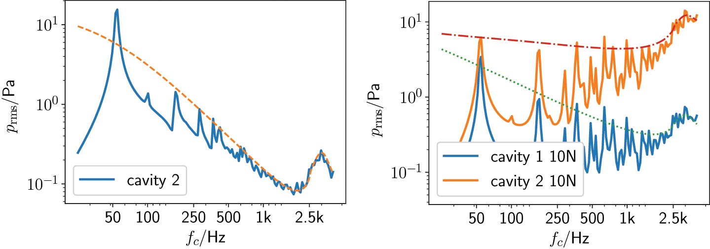
Figure 11.6Pressure in both rooms due to power excitation in cavity 1 (LHS) and force excitation on plate (RHS).

Source: Alexander Peiffer.

11.2.4.3 Step 4.3 – Calculate FE Response due to Energies in SEA Subsystems from Step 4.2

As the external forces were treated by step 4.1, we finally calculate the response of the FEM systems resulting from the reverberant field excitation in each subsystem using (7.43), omitting the deterministic external loads

StartLayout 1st Row 1st Column Start 1 By 1 Matrix 1st Row bold-italic upper S prime Subscript q q comma normal r normal e normal v EndMatrix 2nd Column equals Start 1 By 1 Matrix 1st Row bold-italic upper D prime EndMatrix Subscript tot Superscript negative 1 Baseline left-parenthesis sigma-summation Underscript m Endscripts StartFraction 4 upper E Subscript m Baseline Over pi omega n Subscript m Baseline left-parenthesis omega right-parenthesis EndFraction upper I m Start 1 By 1 Matrix 1st Row bold-italic upper D prime EndMatrix Subscript dir Superscript left-parenthesis m right-parenthesis Baseline right-parenthesis Start 1 By 1 Matrix 1st Row bold-italic upper D prime EndMatrix Subscript tot Superscript negative upper H EndLayout  (11.9)

As the response is calculated in the modal base, the cross spectral density matrix must be converted into the mesh space by

Start 1 By 1 Matrix 1st Row upper S Subscript q q comma normal r normal e normal v Baseline EndMatrix equals Start 1 By 1 Matrix 1st Row normal upper Phi EndMatrix Start 1 By 1 Matrix 1st Row upper S Subscript q q comma r e v Superscript prime Baseline EndMatrix Start 1 By 1 Matrix 1st Row normal upper Phi EndMatrix Superscript upper H  (11.10)

and the rms-velocity results from the diagonal of the above matrix

v Subscript rms Superscript 2 Baseline equals mathematical left-angle diag Start 1 By 1 Matrix 1st Row upper S Subscript q q comma normal r normal e normal v Baseline EndMatrix mathematical right-angle  (11.11)

11.2.5 Step 5 – Adding the Results

In the final step all results are added together for the deterministic systems. The cross spectral density of the plate results from the external excitation and the reverberant load of the connected SEA systems. In Figure 11.7 the rms-velocity of the plate is shown in combination with the SEA result. For the power load case there is no external excitation of the plate, so the reverberant load is the exclusive excitation. The SEA simulation covers only the resonant energy in the plate. This is the reason why both curves don’t agree even at high frequencies, and the resonant SEA solution underestimates the velocity level compared to the FEM system response. When we add the nonresonant motion to the engineering result of the plate using (10.19), both curves agree well above 500 Hz.

In case of the force excitation, the external load response is dominant compared to the reverberant response Sqq,rev. This is obvious, because the reverberant load from the cavities is the indirect feedback of the force exciting the plate. Globally, the results from section 6.4.2.1 are still valid. A point force requires a large modal overlap to fulfil the conditions of a smooth ensemble average. However, above 1kHz the SEA solution is valid.

11.2.5.1 Conlusions

We can perform a Monte Carlo analysis with our test case by generating an ensemble average of different realizations of the plate, and we would get a smoothly averaged result as shown in Shorter and Langley (2005). The example indicates how useful the hybrid theory is, especially for transmission loss calculations, as these cases provide nearly perfect separation between the random systems (cavities) and the deterministic plate. In addition the hybrid theory illustrates the limits of SEA. The modal and resonant dynamics of the plate cannot be modelled by SEA, whereas the high frequency dynamics can be calculated very efficiently without large losses in precision.

This is a rather academic case with simple cavities and a simple flat plate. When real systems or plates with irregularities, beadings, etc. are dealt with there may be more uncertainty in the system, and thus, the random approach becomes a more valid option in comparison to the natural uncertainty of the technical system.

11.3 Trim in Hybrid Theory

For the consideration of trim layers in hybrid theory, the degrees of freedom have to be reorganized in such a way that there are structural and fluid half space degrees of freedom as far as those of the two trim surfaces. In order to keep the derivation simple we consider the plate to be fully covered with noise control treatment.

As the FEM subsystem is modelled by a FEM matrix, a discrete form of the trim layer stiffness is needed. One option is to apply the porous finite element method (PEM) (Allard and Atalla, 2009). We will approximate the stiffness matrix of the noise control treatment by converting the wavenumber transfer matrix into the discrete regular meshed space by an inverse Fourier transform. This assumption is valid for large areas with constant lay-up over the area.

11.3.1 The Trim Stiffness Matrix

In order to cope with the hybrid theory, the acoustic treatment must also be modelled by a a stiffness matrix. This is rather unusual, as, for example, FE implementations are using displacement degrees of freedom for the structure side and pressure degrees of freedom for the fluid side (Doutres et al., 2007) due to the fact that the fluid is represented by pressure degrees of freedom in most solvers.

The trim dynamic stiffness matrix has different sets of degrees of freedom for the left (1) and right (2) side. This suggests writing the matrix in blocked form

StartLayout 1st Row 1st Column Start 2 By 2 Matrix 1st Row 1st Column bold-italic upper D 11 Superscript upper S upper P 2nd Column bold-italic upper D 12 Superscript upper S upper P 2nd Row 1st Column bold-italic upper D 21 Superscript upper S upper P 2nd Column bold-italic upper D 22 Superscript upper S upper P EndMatrix StartBinomialOrMatrix bold-italic w 1 Choose bold-italic w 2 EndBinomialOrMatrix 2nd Column equals StartBinomialOrMatrix bold-italic upper F 1 Choose bold-italic upper F 2 EndBinomialOrMatrix EndLayout  (11.12)

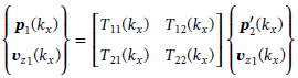
The calculation of the above stiffness matrix is done in two steps: First, the transfer matrix of the infinite layer from section 9.3 is transformed into the stiffness matrix in wavenumber domain.

StartLayout 1st Row 1st Column Start 2 By 2 Matrix 1st Row 1st Column bold-italic upper D 11 Superscript double-prime upper S upper P Baseline left-parenthesis k Subscript x Baseline right-parenthesis 2nd Column bold-italic upper D 12 Superscript double-prime upper S upper P Baseline left-parenthesis k Subscript x Baseline right-parenthesis 2nd Row 1st Column bold-italic upper D 21 Superscript double-prime upper S upper P Baseline left-parenthesis k Subscript x Baseline right-parenthesis 2nd Column bold-italic upper D 22 Superscript double-prime upper S upper P Baseline left-parenthesis k Subscript x Baseline right-parenthesis EndMatrix StartBinomialOrMatrix bold-italic w 1 left-parenthesis k Subscript x Baseline right-parenthesis Choose bold-italic w 2 left-parenthesis k Subscript x Baseline right-parenthesis EndBinomialOrMatrix 2nd Column equals 2nd Row 1st Column Start 1 By 1 Matrix 1st Row bold-italic upper D Superscript double-prime upper S upper P Baseline left-parenthesis k Subscript x Baseline right-parenthesis EndMatrix StartBinomialOrMatrix bold-italic w 1 left-parenthesis k Subscript x Baseline right-parenthesis Choose bold-italic w 2 left-parenthesis k Subscript x Baseline right-parenthesis EndBinomialOrMatrix 2nd Column equals StartBinomialOrMatrix bold-italic upper F double-prime 1 left-parenthesis k Subscript x Baseline right-parenthesis Choose bold-italic upper F double-prime 2 left-parenthesis k Subscript x Baseline right-parenthesis EndBinomialOrMatrix equals StartBinomialOrMatrix bold-italic p 1 left-parenthesis k Subscript x Baseline right-parenthesis Choose bold-italic p 2 left-parenthesis k Subscript x Baseline right-parenthesis EndBinomialOrMatrix EndLayout  (11.13)

Second, this stiffness matrix must be converted into the discrete space. For the approximation of this discrete stiffness matrix, we assume a regular mesh with constant element lengths Δx,Δy. The transfer matrix of infinite layers (9.96)

StartLayout 1st Row with Label StartBinomialOrMatrix bold-italic p 1 left-parenthesis k Subscript x Baseline right-parenthesis Choose bold-italic v Subscript z Baseline Subscript 1 Baseline left-parenthesis k Subscript x Baseline right-parenthesis EndBinomialOrMatrix EndLabel equals Start 2 By 2 Matrix 1st Row 1st Column upper T 11 left-parenthesis k Subscript x Baseline right-parenthesis 2nd Column upper T 12 left-parenthesis k Subscript x Baseline right-parenthesis 2nd Row 1st Column upper T 21 left-parenthesis k Subscript x Baseline right-parenthesis 2nd Column upper T 22 left-parenthesis k Subscript x Baseline right-parenthesis EndMatrix StartBinomialOrMatrix bold-italic p prime 2 left-parenthesis k Subscript x Baseline right-parenthesis Choose bold-italic v Subscript z Baseline Subscript 1 Baseline left-parenthesis k Subscript x Baseline right-parenthesis EndBinomialOrMatrix EndLayout  (9.96)

is to be converted into the stiffness matrix (11.13). The internal pressure p2 must be replaced by the external pressure p2=p2

StartLayout 1st Row 1st Column StartFraction 1 Over bold-italic upper T 21 EndFraction Start 2 By 2 Matrix 1st Row 1st Column bold-italic upper T 11 2nd Column negative 1 2nd Row 1st Column negative 1 2nd Column bold-italic upper T 22 EndMatrix StartBinomialOrMatrix bold-italic v Subscript z Baseline 1 Choose bold-italic v Subscript z Baseline 2 EndBinomialOrMatrix 2nd Column equals 2nd Row 1st Column StartFraction j omega Over bold-italic upper T 21 EndFraction Start 2 By 2 Matrix 1st Row 1st Column bold-italic upper T 11 2nd Column negative 1 2nd Row 1st Column negative 1 2nd Column bold-italic upper T 22 EndMatrix StartBinomialOrMatrix bold-italic w 1 Choose bold-italic w 2 EndBinomialOrMatrix 2nd Column equals StartBinomialOrMatrix bold-italic p 1 Choose bold-italic p 2 EndBinomialOrMatrix EndLayout  (11.14)

and the coefficients of the stiffness matrix in wavenumber domain are hence

StartLayout 1st Row 1st Column bold-italic upper D 11 Superscript double-prime upper S upper P Baseline left-parenthesis k Subscript x Baseline right-parenthesis 2nd Column equals StartFraction j omega bold-italic upper T 11 Over bold-italic upper T 21 EndFraction EndLayout  (11.15)
StartLayout 1st Row 1st Column bold-italic upper D 12 Superscript double-prime upper S upper P Baseline left-parenthesis k Subscript x Baseline right-parenthesis equals bold-italic upper D 12 Superscript double-prime upper S upper P Baseline left-parenthesis k Subscript x Baseline right-parenthesis 2nd Column equals minus StartFraction j omega Over bold-italic upper T 21 EndFraction EndLayout  (11.16)
StartLayout 1st Row 1st Column bold-italic upper D 22 Superscript double-prime upper S upper P Baseline left-parenthesis k Subscript x Baseline right-parenthesis 2nd Column equals StartFraction j omega bold-italic upper T 22 Over bold-italic upper T 21 EndFraction EndLayout  (11.17)

In Figure 11.8 such a treatment connected to a structure is shown. Tournour et al. (2007) proposed a local approximation that assumes that only the opposite nodes are connected. This assumption is valid for very thin layers (hλ), and the block matrices in equation (11.12) are diagonal in that case. It is shown by Peiffer (2018) that this assumption is too strict and a nonlocal approach is required for most treatments.

Figure 11.8 2D sketch of plate with trim.

Source: Alexander Peiffer.

This matrix must be converted into the space domain by inverse Fourier transform. Using the jinc-function approach from Langley (2007) and assuming isotropy in each layer, the transformation becomes simple and implies a finite wavenumber integration.

StartLayout 1st Row 1st Column bold-italic upper D Subscript a b Superscript upper S upper P Baseline left-parenthesis x Subscript i j Baseline comma omega right-parenthesis 2nd Column equals StartFraction normal upper Delta upper A Over 2 pi EndFraction integral Subscript 0 Superscript k Subscript s Baseline Baseline bold-italic upper D Subscript a b Superscript double-prime upper S upper P Baseline left-parenthesis k right-parenthesis upper J 0 left-parenthesis k x Subscript i j Baseline right-parenthesis k d k EndLayout  (11.18)

The transformation is applied to each coefficient of the stiffness matrix with wavenumber arguments

StartLayout 1st Row 1st Column a comma b 2nd Column equals 1 comma 2 3rd Column x Subscript i j 4th Column equals StartRoot x Subscript i Superscript 2 Baseline minus x Subscript j Superscript 2 Baseline EndRoot and k Subscript s Baseline equals StartFraction 2 pi Over StartRoot normal upper Delta x squared plus normal upper Delta y squared EndRoot EndFraction EndLayout  (11.19)

being the projected distance xij between nodes, and the maximum wavenumber ks that can be represented by the spacial sampling of the mesh, respectively. The integral in (11.18) is solved numerically, and the stiffness matrix of the trim is available for further considerations.

11.3.2 Hybrid Modal Formulation of Trim and Plate

The trim constitutes an additional deterministic layer that must be considered in the total stiffness matrix. When a layer of noise control treatment is applied to the right surface, the plate degrees of freedom are shared with those from left side of the trim. The right side of the noise control treatment is connected to the fluid as shown in figure 11.8.

This configuration gives rise to the following block matrix configuration

StartLayout 1st Row left-parenthesis Start 2 By 2 Matrix 1st Row 1st Column bold-italic upper D Subscript s Baseline 2nd Column Blank 2nd Row 1st Column Blank 2nd Column Blank EndMatrix plus Start 2 By 2 Matrix 1st Row 1st Column bold-italic upper D Subscript dir Superscript left-parenthesis 1 right-parenthesis Baseline 2nd Column Blank 2nd Row 1st Column Blank 2nd Column bold-italic upper D Subscript dir Superscript left-parenthesis 2 right-parenthesis Baseline EndMatrix plus Start 2 By 2 Matrix 1st Row 1st Column bold-italic upper D 11 Superscript upper S upper P Baseline 2nd Column bold-italic upper D 12 Superscript upper S upper P Baseline 2nd Row 1st Column bold-italic upper D 21 Superscript upper S upper P Baseline 2nd Column bold-italic upper D 22 Superscript upper S upper P Baseline EndMatrix right-parenthesis StartBinomialOrMatrix bold-italic w 1 Choose bold-italic w 2 EndBinomialOrMatrix equals StartBinomialOrMatrix bold-italic upper F 1 Choose bold-italic upper F 2 EndBinomialOrMatrix EndLayout  (11.20)

adding up to the total stiffness matrix with trim

Start 1 By 1 Matrix 1st Row bold-italic upper D Subscript tot Baseline EndMatrix equals Start 2 By 2 Matrix 1st Row 1st Column bold-italic upper D Subscript s Baseline plus bold-italic upper D 11 Superscript upper S upper P Baseline plus bold-italic upper D Subscript dir Superscript left-parenthesis 1 right-parenthesis Baseline 2nd Column bold-italic upper D 12 Superscript upper S upper P Baseline 2nd Row 1st Column bold-italic upper D 21 Superscript upper S upper P Baseline 2nd Column bold-italic upper D 22 Superscript upper S upper P Baseline plus bold-italic upper D Subscript dir Superscript left-parenthesis 2 right-parenthesis EndMatrix  (11.21)

The coupling loss factor can be calculated when we write (7.27) in block matrix form

eta 12 equals StartFraction 2 Over pi n 1 omega EndFraction sigma-summation Underscript i comma j Endscripts upper I m Start 2 By 2 Matrix 1st Row 1st Column bold-italic upper D Subscript dir Superscript left-parenthesis 1 right-parenthesis 2nd Column Blank 2nd Row 1st Column Blank 2nd Column Blank EndMatrix Subscript i j Baseline left-parenthesis Start 2 By 2 Matrix 1st Row 1st Column bold-italic upper D 11 Superscript upper S upper P Baseline 2nd Column bold-italic upper D 12 Superscript upper S upper P Baseline 2nd Row 1st Column bold-italic upper D 21 Superscript upper S upper P Baseline 2nd Column bold-italic upper D 22 Superscript upper S upper P Baseline EndMatrix Subscript tot Superscript negative 1 Baseline upper I m Start 2 By 2 Matrix 1st Row 1st Column Blank 2nd Column Blank 2nd Row 1st Column Blank 2nd Column bold-italic upper D Subscript dir Superscript left-parenthesis 2 right-parenthesis Baseline EndMatrix Start 2 By 2 Matrix 1st Row 1st Column bold-italic upper D 11 Superscript upper S upper P Baseline 2nd Column bold-italic upper D 12 Superscript upper S upper P Baseline 2nd Row 1st Column bold-italic upper D 21 Superscript upper S upper P Baseline 2nd Column bold-italic upper D 22 Superscript upper S upper P Baseline EndMatrix Subscript tot Superscript negative upper H Baseline right-parenthesis Subscript i j  (11.22)

The above equation can be used as is but leads to double size matrices in this case. The idea is to stay with the plate displacement coordinates and condense the above equation to pure structural coordinates, here w1. Writing equation (11.20) using the block matrix gives

StartLayout 1st Row 1st Column left-parenthesis Start 1 By 1 Matrix 1st Row bold-italic upper D EndMatrix Subscript s Baseline plus Start 1 By 1 Matrix 1st Row bold-italic upper D 11 Superscript upper S upper P Baseline EndMatrix plus Start 1 By 1 Matrix 1st Row bold-italic upper D Subscript dir Superscript left-parenthesis 1 right-parenthesis Baseline EndMatrix right-parenthesis 2nd Column Start 1 By 1 Matrix 1st Row bold-italic w 1 EndMatrix 3rd Column plus Start 1 By 1 Matrix 1st Row bold-italic upper D 12 Superscript upper S upper P EndMatrix Start 1 By 1 Matrix 1st Row bold-italic w 2 EndMatrix 4th Column equals Start 1 By 1 Matrix 1st Row bold-italic upper F 1 EndMatrix EndLayout  (11.23)
StartLayout 1st Row 1st Column Start 1 By 1 Matrix 1st Row bold-italic upper D 21 Superscript upper S upper P EndMatrix 2nd Column Start 1 By 1 Matrix 1st Row bold-italic w 1 EndMatrix 3rd Column plus left-parenthesis Start 1 By 1 Matrix 1st Row bold-italic upper D 22 Superscript upper S upper P Baseline EndMatrix plus Start 1 By 1 Matrix 1st Row bold-italic upper D Subscript dir Superscript left-parenthesis 2 right-parenthesis Baseline EndMatrix right-parenthesis Start 1 By 1 Matrix 1st Row bold-italic w 2 EndMatrix 4th Column equals Start 1 By 1 Matrix 1st Row bold-italic upper F 2 EndMatrix EndLayout  (11.24)

We eliminate w2 in order to express the total stiffness in structural coordinates. Doing this with equations (11.23) and (11.24) leads to
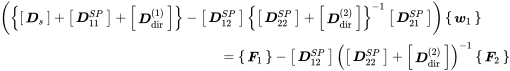
StartLayout 1st Row left-parenthesis left-brace Start 1 By 1 Matrix 1st Row bold-italic upper D Subscript s Baseline EndMatrix plus Start 1 By 1 Matrix 1st Row bold-italic upper D 11 Superscript upper S upper P Baseline EndMatrix plus Start 1 By 1 Matrix 1st Row bold-italic upper D Subscript dir Superscript left-parenthesis 1 right-parenthesis Baseline EndMatrix right-brace minus Start 1 By 1 Matrix 1st Row bold-italic upper D 12 Superscript upper S upper P Baseline EndMatrix left-brace Start 1 By 1 Matrix 1st Row bold-italic upper D 22 Superscript upper S upper P Baseline EndMatrix plus Start 1 By 1 Matrix 1st Row bold-italic upper D Subscript dir Superscript left-parenthesis 2 right-parenthesis Baseline EndMatrix right-brace Superscript negative 1 Baseline Start 1 By 1 Matrix 1st Row bold-italic upper D 21 Superscript upper S upper P Baseline EndMatrix right-parenthesis Start 1 By 1 Matrix 1st Row bold-italic w 1 EndMatrix 2nd Row equals Start 1 By 1 Matrix 1st Row bold-italic upper F 1 EndMatrix minus Start 1 By 1 Matrix 1st Row bold-italic upper D 12 Superscript upper S upper P Baseline EndMatrix left-parenthesis Start 1 By 1 Matrix 1st Row bold-italic upper D 22 Superscript upper S upper P Baseline EndMatrix plus Start 1 By 1 Matrix 1st Row bold-italic upper D Subscript dir Superscript left-parenthesis 2 right-parenthesis Baseline EndMatrix right-parenthesis Superscript negative 1 Baseline Start 1 By 1 Matrix 1st Row bold-italic upper F 2 EndMatrix EndLayout  (11.25)

There is a modified version of the total stiffness matrix

StartLayout 1st Row 1st Column Start 1 By 1 Matrix 1st Row bold-italic upper D Subscript tot Superscript upper S upper P EndMatrix 2nd Column equals left-brace Start 1 By 1 Matrix 1st Row bold-italic upper D Subscript s Baseline EndMatrix plus Start 1 By 1 Matrix 1st Row bold-italic upper D 11 Superscript upper S upper P Baseline EndMatrix plus Start 1 By 1 Matrix 1st Row bold-italic upper D Subscript dir Superscript left-parenthesis 1 right-parenthesis Baseline EndMatrix right-brace minus Start 1 By 1 Matrix 1st Row bold-italic upper D 12 Superscript upper S upper P Baseline EndMatrix left-brace Start 1 By 1 Matrix 1st Row bold-italic upper D 22 Superscript upper S upper P Baseline EndMatrix plus Start 1 By 1 Matrix 1st Row bold-italic upper D Subscript dir Superscript left-parenthesis 2 right-parenthesis Baseline EndMatrix right-brace Superscript negative 1 Baseline Start 1 By 1 Matrix 1st Row bold-italic upper D 21 Superscript upper S upper P EndMatrix EndLayout  (11.26)

which is valid for coordinates {w1} Due to the condensation {F2} is transformed to {w1} degrees of freedom by

StartLayout 1st Row 1st Column Start 1 By 1 Matrix 1st Row bold-italic upper D Subscript tot Superscript upper S upper P EndMatrix Start 1 By 1 Matrix 1st Row bold-italic w 1 EndMatrix 2nd Column equals Start 1 By 1 Matrix 1st Row bold-italic upper F 1 EndMatrix minus Start 1 By 1 Matrix 1st Row bold-italic upper D 12 Superscript upper S upper P Baseline EndMatrix left-parenthesis Start 1 By 1 Matrix 1st Row bold-italic upper D 22 Superscript upper S upper P Baseline EndMatrix plus Start 1 By 1 Matrix 1st Row bold-italic upper D Subscript dir Superscript left-parenthesis 2 right-parenthesis Baseline EndMatrix right-parenthesis Superscript negative 1 Baseline Start 1 By 1 Matrix 1st Row bold-italic upper F 2 EndMatrix 2nd Row 1st Column Blank 2nd Column equals Start 1 By 1 Matrix 1st Row bold-italic upper F 1 EndMatrix plus Start 1 By 1 Matrix 1st Row bold-italic upper D Subscript t r a n s Superscript upper S upper P Baseline EndMatrix Start 1 By 1 Matrix 1st Row bold-italic upper F 2 EndMatrix EndLayout  (11.27)

using the transformation matrix

StartLayout 1st Row 1st Column Start 1 By 1 Matrix 1st Row bold-italic upper D Subscript t r a n s Superscript upper S upper P EndMatrix 2nd Column equals minus Start 1 By 1 Matrix 1st Row bold-italic upper D 21 Superscript upper S upper P Baseline EndMatrix left-parenthesis Start 1 By 1 Matrix 1st Row bold-italic upper D 22 Superscript upper S upper P Baseline EndMatrix plus Start 1 By 1 Matrix 1st Row bold-italic upper D Subscript dir Superscript left-parenthesis 2 right-parenthesis Baseline EndMatrix right-parenthesis Superscript negative 1 EndLayout  (11.28)

Equation (11.27) provides the deterministic equation of motion for displacement degrees of freedom {w1} of the plate. For use in hybrid coupling loss factor equation (7.27), we replace the direct radiation stiffness by an expression that includes the trim. Let us first consider that the trimmed side is the radiating side. The power radiated by the degrees of freedom from side two {w2} is given by

StartLayout 1st Row 1st Column normal upper Pi 2nd Column equals StartFraction omega Over 2 EndFraction upper I m left-brace Start 1 By 1 Matrix 1st Row bold-italic upper F 2 EndMatrix Start 1 By 1 Matrix 1st Row bold-italic w 2 EndMatrix Superscript asterisk Baseline right-brace equals StartFraction omega Over 2 EndFraction upper I m left-brace Start 1 By 1 Matrix 1st Row bold-italic w 2 EndMatrix Superscript upper T Baseline Start 1 By 1 Matrix 1st Row bold-italic upper D Subscript dir Superscript left-parenthesis 2 right-parenthesis Baseline EndMatrix Start 1 By 1 Matrix 1st Row bold-italic w 2 EndMatrix Superscript asterisk Baseline right-brace EndLayout  (11.29)

Reordering of (11.24) and assuming no external forces F2=0 allows transforming {w1} to {w2}

StartLayout 1st Row 1st Column minus left-parenthesis Start 1 By 1 Matrix 1st Row bold-italic upper D 22 Superscript upper S upper P Baseline EndMatrix plus Start 1 By 1 Matrix 1st Row bold-italic upper D Subscript dir Superscript left-parenthesis 2 right-parenthesis Baseline EndMatrix right-parenthesis Superscript negative 1 Baseline Start 1 By 1 Matrix 1st Row bold-italic upper D 21 Superscript upper S upper P EndMatrix Start 1 By 1 Matrix 1st Row bold-italic w 1 EndMatrix 2nd Column equals 2nd Row 1st Column Start 1 By 1 Matrix 1st Row bold-italic upper D Subscript trans Superscript upper S upper P EndMatrix Superscript upper T Baseline Start 1 By 1 Matrix 1st Row bold-italic w 1 EndMatrix equals Overscript symm Endscripts Start 1 By 1 Matrix 1st Row bold-italic upper D Subscript trans Superscript upper S upper P Baseline EndMatrix Start 1 By 1 Matrix 1st Row bold-italic w 1 EndMatrix 2nd Column equals Start 1 By 1 Matrix 1st Row bold-italic w 2 EndMatrix EndLayout  (11.30)

and we get for the radiated power

normal upper Pi equals StartFraction omega Over 2 EndFraction upper I m left-brace Start 1 By 1 Matrix 1st Row bold-italic w 1 EndMatrix Superscript upper T Baseline Start 1 By 1 Matrix 1st Row bold-italic upper D Subscript trans Superscript upper S upper P Baseline EndMatrix Superscript upper T Baseline Start 1 By 1 Matrix 1st Row bold-italic upper D Subscript dir Superscript left-parenthesis 2 right-parenthesis Baseline EndMatrix Start 1 By 1 Matrix 1st Row bold-italic upper D Subscript trans Superscript upper S upper P Baseline EndMatrix Superscript asterisk Baseline Start 1 By 1 Matrix 1st Row bold-italic w 1 Superscript asterisk Baseline EndMatrix right-brace  (11.31)

The term between both {w1} is called the reduced radiation stiffness

StartLayout 1st Row Start 1 By 1 Matrix 1st Row bold-italic upper D Subscript red Superscript upper S upper P Baseline EndMatrix equals Start 1 By 1 Matrix 1st Row bold-italic upper D Subscript trans Superscript upper S upper P EndMatrix Superscript upper T Baseline Start 1 By 1 Matrix 1st Row bold-italic upper D Subscript dir Superscript left-parenthesis 2 right-parenthesis Baseline EndMatrix Start 1 By 1 Matrix 1st Row bold-italic upper D Subscript trans Superscript upper S upper P EndMatrix Superscript asterisk EndLayout  (11.32)

Thus, the radiated power can be calculated with

StartLayout 1st Row 1st Column normal upper Pi 2nd Column equals StartFraction omega Over 2 EndFraction upper I m left-brace Start 1 By 1 Matrix 1st Row bold-italic w 1 EndMatrix Superscript upper T Baseline Start 1 By 1 Matrix 1st Row bold-italic upper D Subscript red Superscript upper S upper P Baseline EndMatrix Start 1 By 1 Matrix 1st Row bold-italic w 1 EndMatrix Superscript asterisk Baseline right-brace equals StartFraction omega Over 2 EndFraction sigma-summation Underscript i comma j Endscripts upper I m left-brace bold-italic upper D Subscript red comma i j Superscript upper S upper P Baseline bold-italic w Subscript 1 comma j Baseline bold-italic w Subscript 1 comma i Superscript upper H Baseline right-brace 2nd Row 1st Column Blank 2nd Column equals StartFraction omega Over 2 EndFraction sigma-summation Underscript i comma j Endscripts upper I m left-brace bold-italic upper D Subscript red comma i j Superscript upper S upper P Baseline right-brace Start 1 By 1 Matrix 1st Row bold-italic upper S Subscript w w comma 1 Superscript asterisk EndMatrix Subscript i j EndLayout  (11.33)

and (11.32) replaces [Ddir(2)] in equation (7.27).

StartLayout 1st Row 1st Column eta 12 Superscript upper S upper P 2nd Column equals StartFraction 2 Over pi n 1 omega EndFraction sigma-summation Underscript i comma j Endscripts upper I m bold-italic upper D Subscript red comma i j Superscript upper S upper P Baseline left-parenthesis Start 1 By 1 Matrix 1st Row bold-italic upper D Subscript tot Superscript upper S upper P Baseline EndMatrix Superscript negative 1 Baseline upper I m Start 1 By 1 Matrix 1st Row bold-italic upper D Subscript dir Superscript left-parenthesis 1 right-parenthesis Baseline EndMatrix Start 1 By 1 Matrix 1st Row bold-italic upper D Subscript tot Superscript upper S upper P Baseline EndMatrix Superscript negative upper H Baseline right-parenthesis Subscript i j EndLayout  (11.34)

From reciprocity (6.112) it follows that the reduced radiation stiffness can also be used for the reverse direction.

StartLayout 1st Row 1st Column eta 21 Superscript upper S upper P 2nd Column equals StartFraction 2 Over pi n 2 omega EndFraction sigma-summation Underscript i comma j Endscripts upper I m bold-italic upper D Subscript dir comma i j Superscript left-parenthesis 1 right-parenthesis Baseline left-parenthesis Start 1 By 1 Matrix 1st Row bold-italic upper D Subscript tot Superscript upper S upper P Baseline EndMatrix Superscript negative 1 Baseline upper I m Start 1 By 1 Matrix 1st Row bold-italic upper D Subscript red Superscript upper S upper P Baseline EndMatrix Start 1 By 1 Matrix 1st Row bold-italic upper D Subscript tot Superscript upper S upper P Baseline EndMatrix Superscript negative upper H Baseline right-parenthesis Subscript i j EndLayout  (11.35)

In addition to the reciprocity argument, the above expression can also be derived using the fact that in the condensed equation of motion (11.27), forces {F2} are converted to {F1} by the transformation matrix [DtransSP].

The diffuse field excitation from side two is then given by

StartLayout 1st Row 1st Column Start 1 By 1 Matrix 1st Row bold-italic upper S Subscript f f comma 11 Superscript left-parenthesis 2 right-parenthesis EndMatrix 2nd Column equals mathematical left-angle bold-italic upper F 1 bold-italic upper F 1 Superscript upper H Baseline mathematical right-angle Subscript upper E Baseline equals mathematical left-angle Start 1 By 1 Matrix 1st Row bold-italic upper D Subscript trans Superscript upper S upper P Baseline EndMatrix bold-italic upper F 2 bold-italic upper F 2 Superscript upper H Baseline Start 1 By 1 Matrix 1st Row bold-italic upper D Subscript trans Superscript upper S upper P Baseline EndMatrix Superscript upper H Baseline mathematical right-angle Subscript upper E Baseline 2nd Row 1st Column Blank 2nd Column equals StartFraction 4 upper E 2 Over pi n 2 left-parenthesis omega right-parenthesis omega EndFraction Start 1 By 1 Matrix 1st Row bold-italic upper D Subscript trans Superscript upper S upper P Baseline EndMatrix upper I m Start 1 By 1 Matrix 1st Row bold-italic upper D Subscript dir Superscript left-parenthesis 2 right-parenthesis Baseline EndMatrix Start 1 By 1 Matrix 1st Row bold-italic upper D Subscript trans Superscript upper S upper P EndMatrix Superscript upper H Baseline 3rd Row 1st Column Blank 2nd Column equals StartFraction 4 upper E 2 Over pi n 2 left-parenthesis omega right-parenthesis omega EndFraction upper I m Start 1 By 1 Matrix 1st Row bold-italic upper D Subscript red Superscript upper S upper P EndMatrix EndLayout  (11.36)

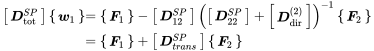
Entering this expression in (7.21) leads also to (11.35). It can be shown that a trimmed surface can be considered in general by using the total stiffness matrix given by

StartLayout 1st Row 1st Column Start 1 By 1 Matrix 1st Row bold-italic upper D Subscript t o t Superscript upper S upper P EndMatrix 2nd Column equals Start 1 By 1 Matrix 1st Row bold-italic upper D Subscript s Baseline EndMatrix plus sigma-summation Underscript m Endscripts Start 1 By 1 Matrix 1st Row bold-italic upper D Subscript dir Superscript left-parenthesis m right-parenthesis EndMatrix EndLayout  (11.37)

using the different expression for trimmed sufaces

StartLayout 1st Row 1st Column Start 1 By 1 Matrix 1st Row bold-italic upper D Subscript dir comma red Superscript left-parenthesis m right-parenthesis EndMatrix 2nd Column equals Start 1 By 1 Matrix 1st Row bold-italic upper D 12 Superscript upper S upper P Baseline EndMatrix minus Start 1 By 1 Matrix 1st Row bold-italic upper D 12 Superscript upper S upper P Baseline EndMatrix left-parenthesis Start 1 By 1 Matrix 1st Row bold-italic upper D 22 Superscript upper S upper P Baseline EndMatrix plus Start 1 By 1 Matrix 1st Row bold-italic upper D Subscript dir Superscript left-parenthesis m right-parenthesis Baseline EndMatrix right-parenthesis Superscript negative 1 Baseline Start 1 By 1 Matrix 1st Row bold-italic upper D 21 Superscript upper S upper P EndMatrix EndLayout

According to equations (11.34) and (11.35), the radiation stiffness must be replaced by the reduced radiation stiffness if there is trim on the surface. The same approach is used for all other expressions used in the hybrid formulation, for example (7.52).

11.3.3 Modal Space

The stiffness matrix must be transformed into the modal space for both sets of degrees of freedom. The transformation reads:

StartLayout 1st Row 1st Column Start 1 By 1 Matrix 1st Row bold-italic w 1 EndMatrix 2nd Column equals Start 1 By 1 Matrix 1st Row normal upper Phi EndMatrix Start 1 By 1 Matrix 1st Row bold-italic w prime 1 EndMatrix 3rd Column Start 1 By 1 Matrix 1st Row bold-italic w 2 EndMatrix 4th Column equals Start 1 By 1 Matrix 1st Row normal upper Phi EndMatrix Start 1 By 1 Matrix 1st Row bold-italic w prime 2 EndMatrix EndLayout  (11.38)

Or, in matrix form when we write all connecting region degrees of freedom in one column vector

StartLayout 1st Row 1st Column StartBinomialOrMatrix bold-italic w 1 Choose bold-italic w 2 EndBinomialOrMatrix 2nd Column equals Start 2 By 2 Matrix 1st Row 1st Column normal upper Phi 2nd Column Blank 2nd Row 1st Column Blank 2nd Column normal upper Phi EndMatrix StartBinomialOrMatrix bold-italic w prime 1 Choose bold-italic w prime 2 EndBinomialOrMatrix EndLayout  (11.39)

The transformation matrix is a block matrix with twice the modal transformation matrix. All system matrices are transformed into modal space by this matrix meaning to apply the modal transformation matrix to every block matrix. All above given matrices are converted to modal space with the usual transformation.

The same is true for the block matrices of the trim leading to:

StartLayout 1st Row 1st Column Start 1 By 1 Matrix 1st Row bold-italic upper D Subscript a b Superscript prime upper S upper P EndMatrix 2nd Column equals Start 1 By 1 Matrix 1st Row normal upper Phi EndMatrix Superscript upper H Baseline Start 1 By 1 Matrix 1st Row bold-italic upper D Subscript a b Superscript upper S upper P Baseline EndMatrix Start 1 By 1 Matrix 1st Row normal upper Phi EndMatrix EndLayout  (11.40)

From the conversion to modal space follows a useful property for evaluating the radiation: the modal radiation efficiency given by

StartLayout 1st Row sigma Subscript n Baseline equals StartFraction 1 Over omega normal upper Delta upper A rho 2 c 2 EndFraction StartFraction upper I m bold-italic upper D Subscript dir Superscript left-parenthesis 2 right-parenthesis Baseline Over normal upper Phi Subscript n Superscript upper H Baseline normal upper Phi Subscript n Baseline EndFraction EndLayout  (11.41)

For configurations with trim the reduced radiation stiffness from equation (11.32) shall be considered.

11.3.4 Plate Example with Trim

We apply this theory to the plate from section 11.2. The panel surface connected to cavity 2 is treated with the 5 cm fiber-mass system from section 10.5.3. With the given theory the transmission loss is calculated and shown in Figure 11.8 in comparison with the SEA result. The agreement between hybrid and SEA is even better than for the untrimmed case. Both approaches start to coincide above 250 Hz in contrast to figure 11.3 where the agreement started around 1 kHz. This is the reason why SEA is considered often as valid even at low frequencies for airborne problems. The dissipation by the noise treatment introduces damping into the system that results in an earlier fulfillment in frequency of the requirements of SEA.

Figure 11.9Transmission loss of small panel with trim, hybrid and SEA solution.

Source: Alexander Peiffer.

Bibliography

  1. Jean-F. Allard and Noureddine Atalla. Propagation of Sound in Porous Media. Wiley, second edition, 2009. ISBN 978-0-470-74661-5.
  2. David Alan Bies, Colin H. Hansen, and Carl Q. Howard. Engineering Noise Control. CRC Press, Boca Raton, fifth edition, 2018. ISBN 978-1-138-30690-5 978-1-4987-2405-0.
  3. Olivier Doutres, Nicolas Dauchez, and Jean-Michel Génevaux. Porous layer impedance applied to a moving wall: Application to the radiation of a covered piston. The Journal of the Acoustical Society of America, 121(1):206, 2007. ISSN 00014966.
  4. R. S. Langley. Numerical evaluation of the acoustic radiation from planar structures with general baffle conditions using wavelets. The Journal of the Acoustical Society of America, 121(2): 766–777, 2007.
  5. Alexander Peiffer. Comparison of the computational expense of hybrid FEM/SEA calculation. In Proceedings NOVEM 2012, Sorrento, Italy, April 2012.
  6. Alexander Peiffer. Hybrid modelling of transmission loss with acoustic treatment. In Fortschritte Der Akustik, pages 50–53, München, Germany, March 2018.
  7. P. J. Shorter and R. S. Langley. Vibro-acoustic analysis of complex systems. Journal of Sound and Vibration, 288(3): 669–699, 2005. ISSN 0022-460X.
  8. Michel A. Tournour, Fumihiko Kosaka, and Hirotaka Shiozaki. Fast Acoustic Trim Modeling using Transfer Admittance and Finite Element Method. In Proceedings SAE 2007 Noise and Vibration Conference, pages 2007–01–2166, May 2007.
..................Content has been hidden....................

You can't read the all page of ebook, please click here login for view all page.
Reset
18.219.48.116