CHAPTER 3
Simulation in ROS
CONTENTS
3.1 Simple two-dimensional robot simulator
3.2 Modeling for dynamic simulation
3.3 Unified robot description format
3.6 Using Gazebo plug-in for joint servo control
3.7 Building mobile-robot model
3.8 Simulating mobile-robot model
INTRODUCTION
This chapter introduces simulation in ROS, starting with a simple two-dimensional mobile-robot simulator and extending to Gazebo–a powerful dynamic simulator. The Unified Robot Description Format (URDF) is introduced for modeling robots suitable for simulation in Gazebo. Controlling wheels or joints of a robot in Gazebo is illustrated in simplified examples. Gazebo
3.1 Simple two-dimensional robot simulator
A helpful place to start the introduction to simulation in ROS is with the Simple Two-Dimensional Robot simulator (STDR). This package is described at http://www.w3.org/1999/xlink, with accompanying tutorials at http://www.w3.org/1999/xlink. If the STDR package is not already installed, it may be installed with the command:

(STDR should already be installed when using the recommended installation scripts accompanying this text). STDR Simple Two-Dimensional Robot STDR may be launched with the command:

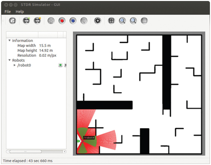
Figure 3.1 Display from STDR launch.
This results in a screen display as shown in Fig 3.1. A small circle in the lower left corner of the maze represents an abstracted mobile robot. The red rays illustrate simulated laser lines from a hypothetical LIDAR sensor. (See http://www.w3.org/1999/xlink for a description of LIDAR sensors.) LIDAR The LIDAR rays extend from the robot out to the first point of reflection in the environment subject to a maximum sensing range. The green cones represent simulated sonar signals. The distance reported by a sonar sensor corresponds to the range to the first sound-reflecting object in the environment within the sensing angle of the sonar (again, subject to a sensing range limitation). Sensor values from the robot simulator are published to topics. The robot subscribes to a command topic, via which the user can control motion of the simulated robot. In fact, running:

shows more than 30 different topics active from the STDR launch. Additionally,

shows 24 services running.
With this simple simulator, one can develop code that can interpret the sensor signals, both to avoid collisions and to help identify the robot’s location in space. Based on sensor interpretation, one can command incremental robot motions to achieve a desired behavior, such as navigating to specified coordinates in the map. We will defer sensory processing for now and focus on controlling the robot’s motion (open loop, without benefit of sensor information). The topic of interest for controlling the robot is /robot0/cmd_vel. The name cmd_vel is (by convention, though not requirement) the topic name used for controlling robots in velocity-command mode. This topic lives within the namespace of /robot0. The cmd_vel topic has been made a subset of /robot0 to allow for launching multiple robots within the same simulation. If (as is typical) a ROS system is dedicated to control a single robot, the /robot0 namespace may be omitted. cmd_vel
We can examine the topic /robot0/cmd_vel with:

which displays:
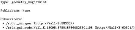
This reveals that the /robot_manager node is listening to this topic, but at present there are no publishers to this topic. Further, we see that messages on this topic are of type geometry_msgs/Twist. We can examine the Twist message with:

which displays:

geometry_msgs Twist
The Twist message contains the equivalent of two vectors: a speed vector (with x, y and z components) and an angular-velocity (rotation rate) vector, also with x, y and z components. This message type is sufficient for specifying arbitrary velocities in space, both translating and spinning or tumbling. It is often useful to have full 6-D command capability, for example for aerial vehicles, submersible vehicles or the end-effector of an arm.
For our two-D mobile robot, only two of these six components are viable. Constraining the motion of the robot to a plan, the robot can only move forward (relative to its own heading) and/or spin about its center. These speed and spin components correspond to the x component of linear velocity and the z component of angular velocity.
We can command a velocity to the robot manually from a terminal by entering:

The above command instructs the robot to move forward at a velocity of 0.5 meters per second (m/s) with constant heading (zero angular velocity). (Note: by default, all units in ROS messages are international standard, meters-kilograms-seconds, or MKS.) As a result of this command, the robot moves forward until it hits an obstacle, as shown in Fig 3.2. Note that the LIDAR rays and sonar cones have changed to be consistent with the new relative positions of reflective surfaces in the robot’s virtual world.
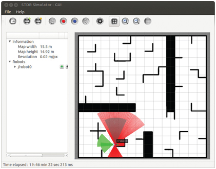
Figure 3.2 STDR stalls at collision after executing forward motion command from start position
The manually entered Twist command is reiterated at 2 Hz, via the option -r 2. However, if the rostopic pub command is halted (with control-C), the robot will continue to try to move with the last Twist command received. We can return the Twist command to zero with:

To get the robot unstuck and allow it to move forward again, a pure rotation command may be issued, e.g. as:


Figure 3.3 STDR after approximate 90-degree counter-clockwise rotation
The only non-zero component of the above command is the z component of the angular velocity. The robot’s z axis points up (out of the plan view) and a positive angular-velocity command corresponds to counter-clockwise rotation. The commanded angular velocity is 0.1 radians per second. Allowing this command to run for approximately 15 seconds corresponds to a rotation of 1.5 radians, or approximately 90 degrees. The resulting pose of the robot is shown in Fig 3.3. The robot has not translated after this command, but it has rotated (as is apparent from the new sensor visualization) to point approximately toward the upper boundary of the map. If the command:

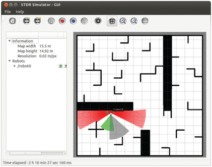
Figure 3.4 STDR stalls again at collision after executing another forward motion command
is issued, the robot will again move forward until it encounters a new barrier, as shown in Fig 3.4. While the manual command-line twist publications illustrate how to control the robot, such commands should be issued programmatically (i.e. from a ROS node). An example node to control the STDR mobile robot appears in the accompanying repository within package stdr_control (under Part II of the repository). This package was created using:

which specifies a dependency on geometry_msgs/Twist, which is needed to publish messages on topic robot0/cmd_vel.
A command publisher node, stdr_open_loop_commander.cpp, was written, starting from a copy of minimal_publisher. The contents of this program appear in Listing 3.1. Line 2 includes the required header file to use the geometry_msgs/Twist message.

A publisher is instantiated on line 7, specifying the command topic and compatible message type:

A sample period is defined on line 9:

and this sample period is used to keep a timer consistent with sleep() calls of a ROS Rate object. A Twist object is defined on line 15:

and lines 17 through 22 show how to access all six components of this message object.
The robot is commanded to move forward 3 m, spin counter-clockwise 90 degrees, then move forward again 3 m. This is done open-loop by commanding speeds for computed durations in lines 32 through 36, 39 through 44, and 48 through 53, thus:

As a result, the robot moves as desired, ending at the final pose shown in Fig 3.5.
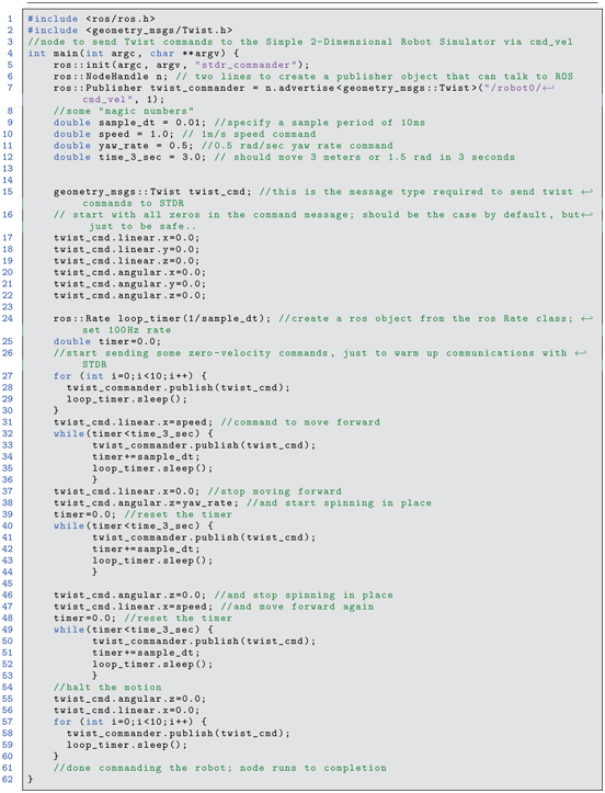
Listing 3.1 stdr_open_loop_commander.cpp: C++ code to command velocities to the STDR simulator
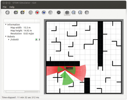
Figure 3.5 STDR final pose after executing programmed speed control
The simple two-dimensional robot simulator may be used to develop more intelligent control code by interpreting sensor values and commanding computed twists that achieve effective reactive behaviors. Approaches to such control will be deferred until sensory-processing techniques have been introduced.
For designing sensor-based behaviors, this level of simulation abstraction may be appropriate, since it easy to operate, requires little computational power and allows the designer to focus on a limited context. This level of abstraction, however, does not include a variety of realistic effects, and thus code developed using this simulator may require additional work with a more general simulator before the code is suitable for testing on a real robot. In addition to the 2-D abstraction, the STDR simulator does not account for sensor noise, force and torque disturbances (including wheel slip), or realistic vehicle dynamics.
The STDR dynamic response can be viewed using rqt_plot. The topic /robot0/odom is useful for analysis, since messages on this topic (of type nav_msgs/Odometry) include the simulated robot’s velocity and angular velocity. (By convention in ROS, a mobile robot should publish its state to an odom topic with message type nav_msgs/Odometry, where the state is based on sensor measurements. Details of the /odom topic will be covered later, in the context of mobile robots.) Figure 3.6 shows the time history of the commanded and actual robot speed and yaw rate. odom topic Odometry nav_msgs
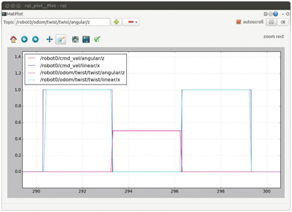
Figure 3.6 STDR commanded and actual speed and yaw rate versus time
Both the speed and spin are commanded with step changes, persisting for 3 seconds within each of the control blocks of the stdr_open_loop_commander.cpp code. The corresponding actual robot speed and yaw rate follow the commands very closely, with almost imperceptible errors due to jitter between when the command is issued and when the robot responds. In reality, the influences of inertia, angular inertia, actuator saturation, wheel friction and servo-controller response would result in very different behavior. Expected non-idealities include ramp-up slew rate limitations, overshoot, and wheel slip. The robot might even fall over due to commanded instantaneous braking. A more realistic controller would ramp up and ramp down the velocity commands to respect dynamic limitations. Appropriate ramping can be implemented to control the STDR simulation, but the necessity of such ramping will not be revealed by STDR, nor can we expect that ramping implemented on STDR will be appropriately tuned for a real robot.
More sophisticated robot simulation requires a sufficiently detailed robot model, including geometry, mass properties, surface contact properties and actuator dynamics. These can be specified using the unified robot description format introduced next.
3.2 Modeling for dynamic simulation
To perform physically realistic dynamic simulations, objects must be specified with sufficient detail. Modeling details are organized within three broad categories: a dynamic model, a collision model and a visual model. (For robots with controlled joints, a kinematic model is also specified.)
Dynamic objects must always include specification of inertial properties. This constitutes the necessary description for an abstract physics model. With an inertial model alone, one can already perform useful simulations. As an example, one could compute the dynamics of a satellite acted on by gravity and thrusters, producing a simulation that incorporates the influences of gravity, centrifugal and Coriolis effects acting on an arbitrary inertia tensor. simulation, dynamic model inertial model kinematic model visual model collision model URDF robot modeling modeling, URDF To compute the dynamics of interacting bodies including colliding objects or a robot grabbing or pushing an object, it is also necessary to compute the forces and moments due to contacts. Simulation of contact dynamics is challenging, and different physics engines address this problem with different methods. The default physics engine used in ROS is Open Dynamics Engine (ODE). Open Dynamics Engine physics engine (See http://www.w3.org/1999/xlink.) This physics engine uses energy and conservation of momentum to deduce the outcome of collisions rather than attempt to detail the very fast dynamics of force profiles during impacts. (As a consequence, this physics engine does a good job of modeling brief collisions, but it suffers from artifacts in simulating sustained contact forces, including wheels on the ground and fingers grasping objects.) To include the dynamic effects of collisions, the simulator must be able to deduce when and where (on each body) contact occurs. It is thus necessary to describe the envelope (boundary description) of 3-D objects in a manner suitable for efficient computation of contact sites. This part of the robot description is a collision model. It can be as simple as a primitive 3-D object description (e.g. a rectangular prism or a cylinder), or it can be a high-fidelity model of a complex surface, typically originating from a CAD model. The surface descriptions are translated to faceted approximations (equivalent to a stereolithography, or STL model, comprised of triangular facets), which is convenient for computing intersections (collisions) between model boundaries. A pragmatic concern with the collision model is that a large number of facets results in slower simulations.
The third category of model description is the visual model, which is used for graphical display purposes. Having a graphical display of the computed dynamics can be very helpful in interpreting results and debugging software development. The visual model is often identical to the collision model, since the visual model also requires a boundary description of each object. It is common, however, for the visual model to be of higher fidelity (e.g. incorporating more facets) than the collision model. Displaying a high-fidelity model is less demanding than computing collisions using a model with a large number of facets.
In the simplest case, the visual model can be identical to the collision model. However, these two categories can include their own options. The collision model, for example, can include specification of surface properties including friction and resilience (which are irrelevant to visual appearance). The visual model may include specifications of color, reflectivity and transparency (which are irrelevant to the collision model).
Some simple model descriptions are contained in the accompanying repository under the package (ROS folder) exmpl_models. Within the subfolder rect_prism of the exmpl_models package, the file model-1_4.sdf is shown in Listing 3.2.

Listing 3.2 rect_prism/model-1_4.sdf: model description of a simple rectangular prism
This file contains a model description using the Simulation Description Format (SDF). simulation description format SDF (SDF; see http://www.w3.org/1999/xlink.) The model description is in XML format and contains three fields: inertial, collision, and visual. The inertial properties include a specification of both the mass (in kilograms) and the moments of inertia (in kilograms- ); explanation of inertial properties will be detailed later in this chapter. The collision and visual models are identical, in this simple case. They both specify a simple box (a rectangular prism) with x, y and z dimensions of 2, 2 and 4 meters, respectively. The rectangular prism has an associated coordinate frame defined to have its origin in the middle of the box, and with x, y, and z axes parallel to the respective specified dimensions.
The simple rectangular prism model is sufficient for performing interesting dynamic simulations. Modeling robots with joint controllers requires additional detail.
3.3 Unified robot description format
URDF Unified Robot Description Format A robot model can be specified using SDF. However, the older unified robot description format (URDF; see http://www.w3.org/1999/xlink) is closely related, and most existing open-source robot models are expressed in URDF. Further, SDF models end up being translated into URDF for use with ROS. This section will thus describe robot modeling in URDF.
A minimal example is introduced here. A good tutorial for more detail can be found at http://www.w3.org/1999/xlink for the rrbot (a 2-degree-of-freedom robot arm). A URDF model can be used as input for dynamic simulation. The dynamic simulator used with ROS is Gazebo (see http://www.w3.org/1999/xlink), which offers alternative choices for physics engines.
3.3.1 Kinematic model
A minimal kinematic model of a single-degree-of-freedom robot in the URDF style is given in Listing 3.3, which is links_and_joints.urdf file in the minimal_robot_description package of our accompanying repository. minimal robot description

Listing 3.3 links_and_joints.urdf: one-DOF robot kinematic description
In Listing 3.3, a robot called one_DOF_robot is defined, consisting of two links and one joint. Descriptions of links and joints are the minimal requirements of a robot definition. These elements are described in XML syntax and may be described in any order in the URDF. It is necessary only that the result is kinematically consistent. robot link robot joint base link
A restriction on URDF files is that one cannot describe closed chains. A URDF will have a single, unique base link, and all other links form a tree relative to this base. This may be a single, open chain (like a conventional robot arm), or the tree may be more complex (such as a humanoid robot with legs, neck, and arms sprouting from a base link on the torso). Closed chains, such as a four-bar linkage, can be “spoofed” in a URDF by making some links kinematically dependent and by introducing virtual actuators; this is adequate for visualization but inaccurate in terms of dynamics. The URDF robot description is not suitable for supporting dynamic simulation of closed-chain mechanisms. open-chain mechanism closed-chain mechanism
An abstraction of a robot model requires only specifying spatial relationships among (solid) links. In the conventional Denavit-Hartenberg representation, this requires only one frame definition per link, Denavit-Hartenberg parameters DH parameters and spatial relations between successive link frames are implied by only four values (three fixed parameters and one joint variable) from parent link to child link. The URDF format departs from this compact description, using up to ten values (nine fixed parameters and one joint variable) instead of the minimum four values. These parameters are described in on-line ROS tutorials; an alternative description of the URDF conventions is offered here.
Each link within a URDF (except for the base link) has a single parent link. However, a link may have multiple child links, e.g. such as multiple fingers extending from the base of a hand, or arms and legs extending from a torso.
Each link has a single reference frame, which is rigidly associated with the link and moves with the link as it moves through space. (The link frame may or may not be located within some part of the physical body of the link, but it nonetheless moves with the link conceptually, as though rigidly attached to some part of the physical body of the link.) In addition to the link frame, there may be one or more joint frames that help to describe how children of the link are kinematically related. (Note: in Denavit-Hartenberg notation, there is no such thing as a joint frame; the joint frame is a URDF construct, which may be convenient in some instances, but also introduces confusing redundancy.)
In Listing 3.3, link1 is the base frame, and link2 is a child of link1. The link frame for the base link is arbitrary—typically a consequence of whatever reference is chosen when describing this link in a CAD system. The respective link frames associated with all other (non-base) links, however, are constrained in their placements by URDF conventions.
For our base link, a joint frame is defined by the lines:
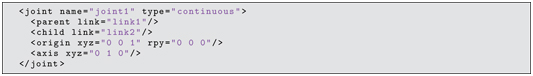
The joint frame is named joint1. This frame is also associated with link1 (the parent link) and moves rigidly with link1. The position and location of this frame are specified by describing the displacement and rotation of the joint frame relative to the parent (link1) reference frame. This spatial relationship is specified by the line:

This specification declares that the origin of the joint1 frame is offset from the link1 frame by the vector [0,0,1], i.e. aligned with the x and y coordinates of the link1 frame, but offset by 1 m in the link1 z direction. (By default, all units in a URDF are MKS.)
We must also specify the orientation of the joint1 frame. In this case, the joint1 frame is orientationally aligned with the link1 reference frame. (i.e. the respective x, y and z axes of these two frames are parallel). This is declared via the specification rpy="0 0 0", which says that the joint1 frame orientation relative to the link1 reference frame is describable with zero roll, pitch and yaw angles.
The joint1 frame is useful as an intermediate frame for describing how link2 is related to link1. The line:

declares that the pose of link2 is related to link1 through a revolute joint. If unspecified, the joint axis of this revolute joint lies colinear with the x axis of the defined joint frame. (Note: this is in contrast to Denavit-Hartenberg convention, in which a joint axis is always defined as a z axis.) In our example, the line:

specifies that the joint axis is not aligned with the joint-frame x axis but is instead colinear with the joint-frame’s y axis. The three components of the axis xyz="0 1 0"/ specification allow for defining an arbitrary joint-axis orientation relative to the joint frame (where the three components specify a unit vector direction in space). Although the joint axis can be oriented arbitrarily, the URDF convention requires that the joint axis pass through the joint-frame’s origin. (Note: orientation of the joint axis specifies more than a line in space; as a direction vector, it also implies a positive sense of rotation for the child link relative to the parent link about a joint axis colinear with this vector.) joint frame link frame
Having defined a joint, the reference frame for the child link follows implicitly. This is an important conceptual constraint (similar to the Denavit-Hartenberg convention for assigning link frames). In the URDF convention, a child link’s reference frame must have its origin coincident with the joint frame that connects the child to the parent. In the simple example provided, the origin of the link2 frame is defined to be coincident with the origin of the specified joint1 frame.
The definition of the orientation of the link2 frame is also constrained by convention, based on the joint1 frame and definition of a home angle for joint home angle joint1. Since a revolute joint joins link2 to link1, link2 can move only by rotating about the joint axis defined revolute joint joint, revolute joint angle within the joint1 frame. When the robot moves with this single degree of freedom, the variable angle is known as the joint angle of joint1. The home angle (or zero angle) for joint1 is a definition, typically chosen to be something convenient (e.g. the 0 reading of the associated rotational sensor, or a convenient alignment that is easy to visualize). When a home angle is chosen, the child link’s reference frame follows. It is defined to be coincident with its parent’s joint frame. That is, if one puts link2 in the defined home position relative to link1, the value of the joint1 angle will be defined to be zero at this pose, and the link2 reference frame will be identical to the joint1 reference frame at this pose. At any other (i.e. non-zero, non-periodic) values of the joint1 angle, the joint1 and link2 frames will not be aligned (although their respective origins will remain coincident).
Our example URDF file thus defines a link frame for each link and how these link frames are constrained to move relative to each other. We can check whether our URDF file is consistent by running:

We can either run this from the minimal_robot_description directory, or provide a path as part of the filename argument to check_urdf. The output produced is: check_urdf The output produced is:

This confirms that our file has correct XML syntax and that the robot definition is kinematically consistent.
To this point, our URDF is consistent, but it only defines the constrained spatial relationship between two frames. For simulation purposes, we need to provide more information: a visual model, a collision model and a dynamic model.
3.3.2 Visual model
visual model Our minimal kinematic model is augmented with visual information in Listing 3.4 (which also appears in the package minimal_robot_description as file one_link_description.urdf in our associated code repository).
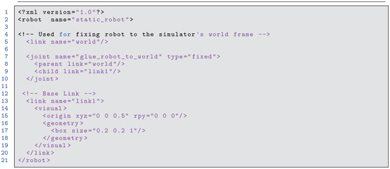
Listing 3.4 one_link_description.urdf: one-link model with visual description
For simulation purposes, a world frame with a ground plane will be defined, and we can place link1 fixed in the world by defining a static joint, lines 7 through 10:
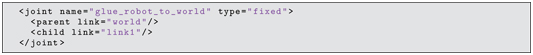
In defining joint glue_robot_to_world, the joint type is specified as fixed, which means our link1 joint, fixed fixed joint will have a static relationship with respect to the world frame. Further, since we did not specify the x,y,z or r,p,y coordinates of the joint frame, the default values (all 0’s) are applied, and our link1-frame is thus defined to be identical to the world frame.
Within the link1 definition, in the sub-section inside the visual tags, lines 16 through 18

define a 3-D box entity with dimensions 0.2 by 0.2 by 1.0 meters. For this simple 3-D primitive (essentially identical to our earlier rect_prism model), a model frame is defined with origin at the center of the box, and x ,y ,z axes along the specified dimensions 0.2, 0.2, 1.0. This entity can be used to define the visual appearance of link1. (More commonly an entire CAD file is referenced to define each robot element, but simple 3-D primitives such as box are useful for quick models and for simple illustration of concepts.)
Although we have defined a link1 frame (which is coincident with the world frame), we also need to define a visual frame for link1, such that our visual model (the box) appears in the correct location. Our link1 frame has its origin at the level of the ground plane, whereas our box entity has its origin in the center of the box. We wish to place the appearance of the box such that it appears to sit on one (square) face (i.e. with this face coplanar with the ground plane) and with the long dimension of the box (the visual frame z axis) pointing up (i.e. normal to the ground plane and parallel to the z axis of the world frame). This is accomplished with line 15:

which specifies that the box frame axes are parallel to the respective link1 frame axes, but that the box frame origin is elevated (offset in the link1 frame z direction) by 0.5 m.
We cannot test our visualization in our simulator yet until we augment the model with additional, dynamic information.
3.3.3 Dynamic model
dynamic model model, dynamic inertial model model, inertial For our robot model to be consistent with a physics engine, we must define mass properties for every link in the system. (Although it should not be necessary conceptually, a dynamic model is required even for link1, which we intend to fix rigidly to the ground plane.) Our one-link model, augmented with mass-property information, is shown in Listing 3.5.

Listing 3.5 one_link_w_mass.urdf: one-link model with visual and inertial descriptions
Within the tags of the link1 description, the additional lines 20 through 27 describe the mass properties:
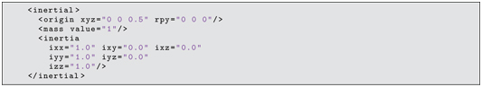
In the inertial field, one specifies the mass of the link (here, set to 1 kg) and the coordinates of the center of mass (here, xyz="0 0 0.5"). The coordinates of the center of mass are specified in the link1 frame. For our box example, if the box has uniform density, the center of mass will be in the center of the box, which is 0.5 m above the link1 frame.
Specifying rotational inertia properties is more complex. Specification of rotational inertia requires defining a coordinate frame with respect to which the inertial properties are computed. With respect to this inertial frame, the components of a matrix inertia tensor may be computed as: model, inertial frame inertial frame
1
where is the density of material at location (x, y, z), and the integral over volume V is defined as the volume of all material comprising the rigid link of interest. The matrix is always symmetric, and thus there are only six values to specify. For simple shapes, this moment of inertia tensor is easy to compute. inertia tensor Many common shapes have published tabulated values. The inertia tensor can be difficult to compute for complex link shapes. If the link is detailed in a CAD program, the CAD program typically can compute the inertia tensor numerically.
Note that the matrix will have different numerical components for different positions and/or orientations of the inertial reference frame. In a URDF, the origin of the inertial frame is always coincident with the center of mass model, center of mass (which is typically convenient in dynamics). It is sometimes convenient to define the orientation of this inertial frame to be aligned with some axes of symmetry, which simplifies specification of inertial components. In the present case (and often in URDFs) the inertial frame is simply chosen to be parallel to the link frame (as specified by the rpy values in origin xyz="0 0 0.5" rpy="0 0 0"/ ).
With respect to the defined reference frame, the rotational inertial components can be specified in the URDF as in lines 23 through 27. The terms of are labeled in the URDF as ixx = , ixy = , ixz = , iyy = , iyz = and izz = .
Ideally, these values will be a close approximation to the true inertial components of the actual links. One should attempt to at least estimate these values roughly. It is important, though, that neither the mass nor the diagonal components of inertia be assigned a value of 0. The physics engine will have divide-by-zero numerical problems trying to simulate the dynamics of massless or inertialess objects.
For our single-link URDF, the mass properties have been assigned to unity (1 kg mass, and 1 rotational inertia about each of the x, y and z principal axes). The inertial values are not realistic for a uniform rectangular prism. However, since this link will be fixed to the ground plane, the accurate mass values will not be a concern.
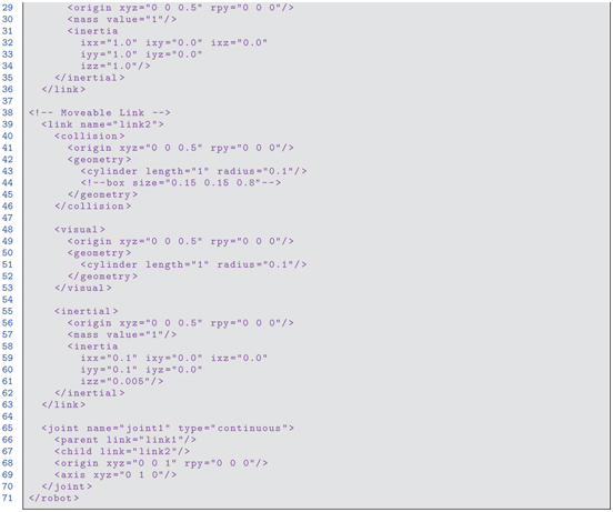
At this point, our model is boring (a static, rectangular prism). Nonetheless, it is a viable URDF that may be loaded into a simulator. This will be deferred, though, until our model becomes more interesting by adding a movable link. Listing 3.6 combines our initial kinematic model with visual and inertial properties.


Listing 3.6 minimal_robot_description_wo_collision.urdf: one-DOF robot URDF description
In Listing 3.6, visual and dynamic models are defined for two links. The joint between these links, joint1, could include additional properties, e.g. to model viscous or Coulomb friction. Further, joint limits and actuator torque limits may be specified. However, the minimal model that we have is adequate for simulating robot dynamics subject to specified joint (actuator) torques and the influence of gravity.
The visual model for link2 is defined on line 36:

as a cylinder of length 1 m and radius 0.1 m. The inertial properties for link2 are specified as mass = 1 kg, ix = iyy = 0.1 and izz = 0.005. These values are reasonable approximations. For a thin rod of uniform density, mass m and length l, the rotational inertia about its x or y axis is . The assigned values have been rounded up to 0.1 . The inertia of this rod spinning about its cylindrical axis is , which evaluates to the assignment of izz = 0.005 .
As with the box entity, the cylinder entity’s reference frame has its origin in the middle of the cylinder. The z axis of this visualization frame points along the cylinder’s major axis.
As introduced in Subsection 3.3.1, the link2 frame is defined to be coincident with the joint1 frame when the angle of joint1 is in its home ( ) position. The reference frame of our visual model is specified relative to the link2 frame in line 34: origin xyz="0 0 0.5" rpy="0 0 0"/ . That is, the visual frame is aligned with the link2 frame (rpy="0 0 0"), but the origin of the visual frame of link2 is offset from the link2 reference from by 0.5 m along the link2 z axis (xyz="0 0 0.5"). As with our box visual description, this 0.5 m offset locates the geometric (visual) model such that one endcap of the model coincides with a joint origin (in this case, joint1).
In the home position, the link2 frame is aligned with the joint1 frame. With our choices, the home position of our one-DOF, two-link robot corresponds to link2 pointing straight up.
3.3.4 Collision model
Our minimal robot description so far has included a kinematic model, an inertial model and a visual model. Motion of our robot will depend on forces and moments exerted on the robot. The dynamics engine of our simulator will enforce the kinematic constraints (e.g. how link2 can move with respect to link1) and will compute angular accelerations of link2 about joint1. These accelerations will be due to effects including gravity, joint torque exerted by an actuator (once we have defined an actuator), and possible collisions with other bodies. To include the influence of contact forces (e.g. due to collisions), we must include a collision model in our URDF. collision model model, collision
A collision | tag defines the region in which the collision model is defined in the URDF. Our one-DOF URDF with collision properties appears in Listing 3.7 (which also appears in the package minimal_robot_description as file minimal_robot_description.urdf in our associated code repository).

Listing 3.7 minimal_robot_description.urdf: one-DOF robot URDF description
In Listing 3.7, the collision models define the geometric detail corresponding to a “skin” on the links. The collision model is used to compute intersections between solids within a world model; such collisions lead to interaction forces and torques at the points of contact.
Often, the collision model is identical to the visual model (and this is the case in Listing 3.7). However, collision checking can be a computationally intensive process, and therefore the collision model should be as sparse as possible. This can be done by reducing the number of triangles in a tessellated surface model, or by creating a primitive collision model based on geometric solids, e.g. rectangular prisms, cylinders or spheres.
Another concern is that a collision model that does not offer adequate clearance between the links can result in simulation instability, as the simulator repeatedly determines that the links are colliding with each other. For our crude model, we will set the collision model of link2 to be identical to the visual model of link2—a simple cylinder. However, we will set the collision model of link1 to be a shorter box, thus providing clearance for link2.
Since link1 is stationary, fidelity of its collision model is not a concern for computing dynamics of this minimal robot. However, if this model were part of a finger, one would care about how this link contacts objects to be grasped. Alternatively, if there were additional robots in the virtual world, one would care about how these robots might collide with link1 of this minimal robot, as such collisions would affect the dynamics of the other robots.
Our one-DOF minimal robot URDF now contains kinematic, inertial, visual and collision information. We next introduce the Gazebo simulator, which can perform dynamic simulations of robots based on URDF specifications.
3.4 Introduction to Gazebo
Gazebo is the simulator used with ROS Gazebo (see http://www.w3.org/1999/xlink). Gazebo offers options for alternative physics engines, with a default of ODE (Open Dynamics Engine). The Gazebo simulator consists of two parts: a server (which runs as process gzserver) and a client (which runs as process gzclient). The client process presents a graphical display and human interface. However, Gazebo can be run “headless” if a visual display is not needed. gzserver gzclient
An impressive and valuable capability of Gazebo is that it can simulate sensors as well as dynamics, including force sensors, accelerometers, sonar, LIDARs, color cameras, and 3-D point-cloud sensors. Description of camera simulation will be deferred to Part III.
Gazebo simulations require a world model in addition to one or more robot models. The world model may contain details of terrain, buildings, barriers, tables, graspable objects, and additional active entities, including swarms of robots. To start simple, however, we consider our minimal robot in a minimal world. world model
A common default world model consists only of a flat ground plane oriented perpendicular to the direction of gravity. To start Gazebo with this empty world model, run:

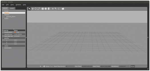
Figure 3.7 Gazebo display of empty world with gravity set to 0
empty world This starts a launch file called empty_world.launch from the ROS package gazebo_ros. The result of this command is to start both the gzserver and the gzclient, presenting a Gazebo display of an empty world (except for a ground plane). The Gazebo window will appear as in Fig 3.7. Along the bottom bar of the Gazebo simulator are some controls and displays. Run and pause buttons allow the user to suspend a simulation and resume it at will. The real time factor display indicates the efficiency of Gazebo, real-time factor the simulation. Gazebo will (by default) try to simulate the robot(s) in the virtual world in real time. If the host computer is not able to keep up with the required computations to achieve real time, the simulator will slow down, resulting in an apparent slow-motion output. If the real time factor is unity, the simulation is equivalent to real-time dynamics; if this factor is e.g. 0.5, the simulation will take twice as long as reality.
On the left side of the Gazebo display, as shown in Fig 3.7, are tabs labeled “World” and “Insert.” The World tab contains the Gazebo, menus option Physics. This element has been expanded and displays various properties, including the gravity item. The gravity item has also been expanded, revealing the numerical values for its x, y and z components. In this example, the z component was changed from its initial value of to 0 (which is done by clicking on the the displayed value and editing it). With gravity set to zero, models can float in space indefinitely, whereas when gravity has a negative z component, models will fall to the ground plane. gravity in Gazebo
Also within the Gazebo window’s World tab is a Models menu, which allows one to inspect the spatial and dynamic properties of all models within the simulation. At this point, the only model in the simulation is a ground plane. We can add models to the simulation in multiple ways. Using the Insert tab, one can select any of the pre-defined models displayed in the model list to be inserted in the simulation. The list of available models will include on-line models in Gazebo’s database, as well as models defined locally that reside within the (hidden) directory /.gazebo. inserting models in Gazebo Gazebo, inserting models
Alternatively, one can load a model into Gazebo manually by invoking a Gazebo node with a path to a model. For example, first navigate to the directory /ros_ws/src/learning_ros/exmpl_models/rect_prism, then enter the following command:

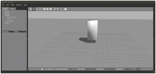
Figure 3.8 Gazebo display after loading rectangular prism model
Gazebo, spawn model spawn model in Gazebo Our simple, rectangular prism model will be loaded into Gazebo, and the display will appear as in Fig 3.8. We can remove this model by clicking on it, then pressing the delete key.
Alternatively, the prism can be loaded with specified world coordinates. For example, the command:

loads the prism with its coordinate frame located 4 m above the ground plane.
Instead of navigating to the model directory to load models, one can include the full path to the model location. This is made somewhat more general with use of the environment variable ROS_WORKSPACE. The following command loads the model using an explicit path:

ROS_WORKSPACE
It can be more convenient to ask ROS to find the package in which the model resides, which can be done with , e.g. as with the following command:

Since direct commands can be tedious to type in, it is typically more convenient to enter the commands in a launch file, then invoke the launch file to load models. An example is in exmpl_models/launch/add_rect_prism.launch. The contents of this file are:

roslaunch, spawn model spawn model from roslaunch The syntax is similar to the command line, though with variations. Within a launch file, one finds ROS packages using instead of . This launch file can be invoked from any directory with:

This command finds the package exmpl_models, implicitly looks in the subdirectory launch, and invokes the launch file add_rect_prism.launch. This launch file loads the rectangular prism model into Gazebo with initial coordinates of . With gravity off, this model remains stationary, floating above the ground plane.
A second simple model (a cylinder) can be added with a similar launch file:

which results in the Gazebo display in Fig 3.9. Note that the Models menu now includes rect_prism and cylinder.

Figure 3.9 Gazebo display after loading rectangular prism and cylinder
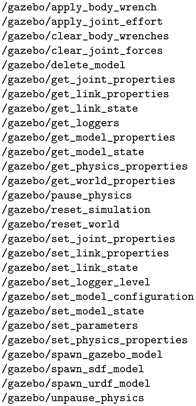
At this point, we have confirmed that our models are syntactically correct, present the expected visual displays, and contain the minimum requirements to be compatible with Gazebo simulation. More interestingly, dynamic simulation can be observed by giving these models an initial velocity that results in collision, from which we can observe behavior of the physics engine. To initialize our models with a non-zero velocity and angular velocity, we can use a service of Gazebo. Running:

shows 30 services running, one of which is /gazebo/set_model_state. Examining this service with

Gazebo set model state SetModelState shows that the service message expects an argument, model_state, of type gazebo_msgs/SetModelState. Looking in the gazebo_msgs/srv directory, one finds the service message description SetModelState.srv, the contents of which is:

which confirms that the request field of this service message contains a field called model_state of type gazebo_msgs/ModelState.
The message type gazebo_msgs/ModelState can be examined with:

which displays details of this message type to be:

A model state can be set using a manual command. An example is:

setting model state in Gazebo This command specifies the model name to be our rectangular prism, and it commands the component of the angular velocity to be 1.0 rad/sec. Implicitly, all other components of position, orientation, linear velocity and angular velocity are set to 0. The syntax for specifying components of a message type is YAML. (See http://www.w3.org/1999/xlink for details on using YAML within a ROS command line.) YAML
Since the YAML syntax can become tedious (and error prone for direct typing), it can be more convenient to set the model state programmatically. An example of how to do this is contained in the package example_gazebo_set_state in the source code (node) example_gazebo_set_prism_state. setting model state from program
Key lines of this node include:

A compatible service message is instantiated with the line:

Components of this message are filled in, e.g. as:

which specifies the model for which the state is to be set, and:

which specifies a component of angular velocity to be 1.0 rad/sec. Similarly, all components of position, orientation, translational velocity and angular velocity can be specified. After the service message is populated, it is sent to the Gazebo service to set the specified model state with:

This program can be run by entering:

which causes the prism to rotate about its direction. After a single service call, this program concludes. The objects subsequently evolve in time according to their twist vectors.
By using the initial conditions within the launch files for loading a prism and a cylinder, then invoking example_gazebo_set_prism_state, the prism will begin spinning and translating, eventually colliding with the cylinder. This collision results in a change in momentum (including angular momentum) of both objects. The states of the models can be observed with:

Before the models collide, this will show that the cylinder has zero twist, but the prism has an angular velocity about its direction of 0.02 m/sec. After the models collide, they both have altered translational and rotational velocities. However, it can be shown that the total system linear momentum and system angular momentum are preserved. (Momentum before collision equals momentum after collision.) This illustrates that the physics engine behaves as expected. Although the objects may be translating and tumbling in a complex way after collision, the system momentum is conserved.
Robot models can be inserted and dynamically modeled in a similar fashion, although the model and its stimulus are more complex. To import our minimal robot model, in a separate terminal, navigate to the minimal_robot_description package and enter:

spawn model from file This invokes the spawn_model node from the gazebo_ros package with three arguments: declaration that the input file is in URDF format, specification of the URDF file name to be loaded, and a model name to assign to the loaded file in Gazebo. This node will run to completion, resulting in inserting the named URDF file into the simulator. The result appears as in Fig 3.10. The figure verifies that we have an upright, rectangular prism for link1 and a cylindrical link2. The coordinate frames for link1 and link2 are illustrated as well, where the red axes are axes. The green circle about the link2 axis indicates that this vector is also a joint axis (the axis of joint1). This display was enabled via the top menu bar of the Gazebo display by enabling view- Joints. The Gazebo menus offer a variety of additional options that can be convenient for visualizing simulations, including centers of mass and contact forces.

Figure 3.10 Gazebo display of two-link, one-DOF robot URDF model
The command rosrun gazebo_ros spawn_model ... can be run alternatively from a launch file. spawn model from launch file For future interaction with ROS nodes and sensor displays, it will be convenient to first load the robot model onto the parameter server, then spawn the model into Gazebo from the parameter server. This will assure that ROS nodes and Gazebo refer to the same details of the robot model. This is accomplished with the example launch file in package minimal_robot_description, minimal_robot_description.launch, which can be run with:

(If the robot has already been spawned in Gazebo, this will generate an error, due to spawning two identical models.) The contents of this launch file are:
spawn model from parameter server The first subfield in this launch file puts a copy of the robot model on the parameter server, and the second field spawns the model into Gazebo using the model drawn from the parameter server. After running this launch file, it can be verified that the robot model is on the parameter server. Running rosparam list shows an item called robot_description on the parameter server. Running rosparam get /robot_description displays the contents of this item, which contains the entire URFD specifications from minimal_robot_ description.urdf. In the future, it will also be convenient to include start-up of joint controllers in the same launch file, which may include specifications of joint control parameters placed on the parameter server as well. robot_description
Models can also be inserted into Gazebo interactively via the Insert tab in the Gazebo GUI, which can be convenient for constructing variations on the virtual world for experiments with the robot. A variety of models are available on-line to import. Additionally, Gazebo will look in the (hidden) user directory called .gazebo for available models; the .gazebo directory typically resides in the user’s home directory. Robots can be spawned into Gazebo in this fashion as well, although it is more useful to do so via the parameter server for better ROS integration.
With Gazebo running, entering:

reveals that the active topics include:
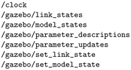
Gazebo messages
Entering:

shows that the following Gazebo services are active: Gazebo services Running:

displays updates of the 6-D pose and 6-D velocity of each link in the system. With the minimal robot spawned into Gazebo, the initial part of the echo display looks like:
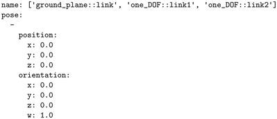
The output declares that there are three links in the system (including the ground plane). The position and orientation of every link and the linear and angular velocity vectors are given. For the simulation at present, these values are boring. All velocities are zero, and all links are aligned with the world frame (except for link2 being elevated by 1.0 m).
The initial pose in this scene is the home pose, corresponding to link2 straight up. In Fig 3.10, link2 is precariously balanced at an unstable equilibrium point. There is no joint controller keeping it upright, and it may unexpectedly tip over, tilting about the joint1 axis.
To make our robot more interesting, a joint controller is needed. The joint controller can integrate with Gazebo, obtaining joint angles and inducing joint torques, simulating a servoed actuator.
3.5 Minimal joint controller
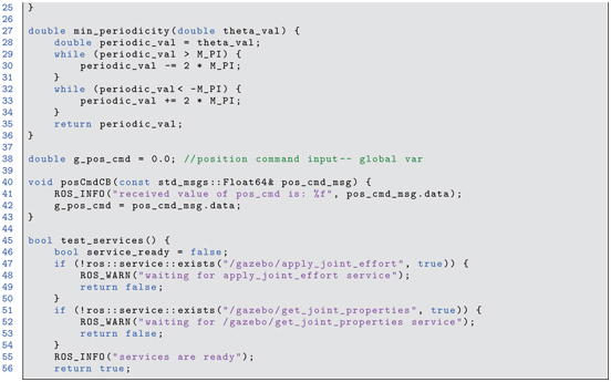
joint controller minimal joint controller An important connection between Gazebo and ROS is how controls are exerted using joint actuator commands and joint displacement sensors. For purposes of illustrating this interaction, a minimal joint controller ROS node is presented. The source code minimal_joint_controller.cpp (in the minimal_joint_controller package) is described here, which interacts with Gazebo and creates a ROS interface (similar to constructing the bridges necessary to interact with a real robot).
Please note that the example controller described here normally would not be used. For a physical robot, the proportional-plus-derivative (PD) controller would be contained within dedicated control hardware. Similarly, for Gazebo, there are pre-defined Gazebo plug-ins that perform the equivalent of the present joint controller example. (See http://www.w3.org/1999/xlink for a tutorial on how to write Gazebo plug-ins.) Gazebo plug-in Thus, you would not need to use the minimal_joint_controller package; this is presented only to illustrate the equivalent of what a Gazebo controller plug-in performs, using concepts already introduced. A disadvantage of using the present controller code relative to a Gazebo plug-in is that the example code incurs additional computational and bandwidth loads of serialization, de-serialization and corresponding latency in message passing, which can be critical in high-performance control implementations.
The contents of minimal_joint_controller.cpp appear in Listings 3.8 (preamble and helper functions) and 3.9 (main program).
Listing 3.8:
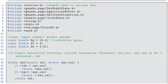
Listing 3.8 minimal_joint_controller.cpp: minimal joint controller via Gazebo services (preamble and helper functions)

Listing 3.9 minimal_joint_controller.cpp: minimal joint controller via Gazebo services (main program)
The example controller in minimal_joint_controller.cpp interacts with Gazebo via service clients of the services /gazebo/get_joint_properties and /gazebo/apply_joint_effort. In lines 36 through 41, the get_joint_properties apply_joint_effort helper function test_services() (lines 45 through 57) is used to make sure the Gazebo services are available, after which corresponding service clients are instantiated (lines 71 through 74). Compatible service messages are instantiated in lines 76 and 77. We can examine the operation of these respective Gazebo services manually.
To examine Gazebo’s services, make sure the minimal robot is running, by first starting Gazebo:

and loading the robot model with:

The Gazebo service /gazebo/get_joint_properties can be examined manually by entering:

which results in the following example output:

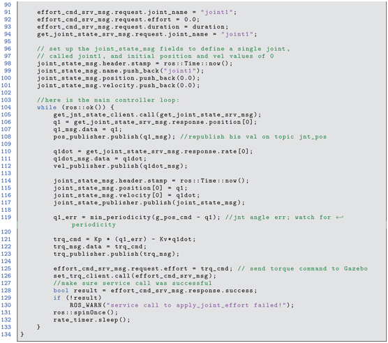
From this service, we can obtain the state of joint1, which includes the joint position and the joint (angular) velocity. The service client of this service, get_jnt_state_client, joint state makes such calls repeatedly in the control loop to obtain the joint position and velocity from the dynamic simulator.
The service client of /gazebo/apply_joint_effort, set_trq_client, sets fields in the corresponding service message for joint_name to joint1 and effort to a desired joint torque, enabling the controller node to impose joint torques on joint1 of the simulated robot.
A subscriber to the topic pos_cmd is also set up (line 83), ready to accept user input for desired joint1 position values via callback function posCmdCB (lines 40 through 43).
The main loop of our controller node does the following:
- Obtains the current joint position and velocity from Gazebo and republishes these on topic joint_states (lines 104 through 117)
- Compares the (virtual) joint sensor value to the commanded joint angle (from the pos_cmd callback), accounting for periodicity (line 119)
- Computes a PD torque response (line 121)
- Sends this effort to Gazebo via the apply_joint_effort service (lines 125 and 126)
The minimal controller node can be started with the command:

Initially, there is no noticeable effect on Gazebo, since the start-up desired angle is 0, and the robot is already at 0 angle. However, we can command a new desired angle manually from the command line (and later, under program control) with the command:
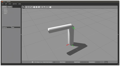
Figure 3.11 Gazebo display of minimal robot with minimal controller

Figure 3.12 Transient response of minimal robot with minimal controller

which commands a new joint angle of 1.0 radians. The robot then moves to the position shown in Fig 3.11. We can record the dynamic response of an input command by plotting the published values of joint torque, velocity and position, using rqt_plot. Enter the command:

then add topics of /jnt_pos/data, /jnt_trq/data and /jnt_vel/data. The plot in Fig 3.12 shows the transient response, starting from a position command of 1.0, then responding to a new command of 2.0. rqt_plot As shown, the initial joint angle is larger than the commanded 1.0. This is due to a low feedback proportional gain and the influence of gravity, causing droop relative to the desired angle. At approximately is required to hold the link against gravity.
To illustrate the influence of contact dynamics, an additional model is added to Gazebo, as shown in Fig 3.13. Here, a cafe table (from a list of pre-defined models) is added using the Insert menu of Gazebo. Gazebo offers the user the capability of moving the table to a desired location, which was chosen here to be within reach of the robot.

Figure 3.13 Gazebo display of minimal robot contacting rigid object
Next, the robot was commanded to position 0 (straight up), then commanded to position 2.5, which is unreachable with the table in the way. The transient dynamics from this command are shown in the Fig 3.14. The collision model of the link and the collision model of the table are used by Gazebo to detect that contact has occurred. This results in a reaction force from the table to the robot (and from the robot to the table). As a result, the robot does not reach its goal angle, and equilibrium occurs with the robot’s joint actuator exerting an effort downward on the table, while struggling to reach the desired angle of 2.5 rad. Gazebo, collisions
The ability to move models in Gazebo under program control can have useful applications in performing simulations in dynamic virtual worlds. As noted, though, simulating joint controllers in Gazebo is better performed using plug-ins, as described next.
3.6 Using Gazebo plug-in for joint servo control
A Gazebo plug-in can run at the full rate of the Gazebo simulator (1 kHz, by default), without the overhead and associated latency of message passing. ROS controllers in Gazebo are intended to be constructed with interfaces identical to actual hardware as well as dynamic behavior in simulation that emulates dynamic behavior of actual hardware. Further, the ROS packages and example controllers were constructed with anticipation of growth and generalization. Unfortunately, this resulted in a fair amount of complexity in creating and simulating models of joint controllers. Further, multiple additional packages are required (including, for example, with the Indigo ROS release: ros-indigo-controller-interface, ros-indigo-gazebo-ros-control, ros-indigo-joint-state-controller, and ros-indigo-effort-controllers). These packages are not installed automatically, even with the desktop-full ROS installation. If you installed ROS using the setup scripts accompanying this text (at http://www.w3.org/1999/xlink), these control packages will already be installed. If you installed ROS manually with the desktop-full option, you will need to install the ros-controller packages (as admin) with:

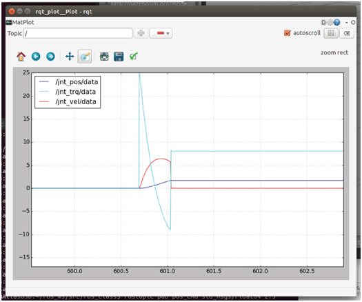
Figure 3.14 Contact transient when colliding with table
Gazebo, control plug-in ros_controllers libgazebo_ros_control plug-in effort control joint transmission A good example to follow regarding ROS control is the rrbot tutorial, which can be found at http://www.w3.org/1999/xlink.
The process for incorporating ROS joint controllers as a Gazebo plug-in requires the following steps:
- Edit the joint fields to specify torque and joint limits in the URDF file
- Add a transmission field to the URDF, one for each joint to be controlled
- Add a gazebo block in the URDF to bring in the libgazebo_ros_control.so controller plug-in library
- Create a controller parameter YAML file that declares the controller gains
- Modify the launch file to put the control parameters on the parameter server and start the controllers running
These steps are illustrated here, revisiting our minimal robot specification. Within the package minimal_robot_description, a modified URDF file, minimal_robot_description_w_jnt_ctl.urdf, contains the additions necessary for ROS joint control. This model file is largely identical to our previous minimal robot URDF, Listing 3.7, and thus it is not repeated in full here. The important additions within minimal_robot_description_w_jnt_ctl.urdf exist within three blocks.
First, the previous joint1 block is modified as follows:

revolute joint joint, revolute joint, continuous prismatic joint joint, prismatic joint, limits This block shows a new type of joint and additional parameters. The revolute joint type is more appropriate than continuous for a robot arm, since robot joints typically have limited range of motion (in contrast to joints for wheels). Another common joint type is prismatic, for joints that extend and retract. (For more detail on joint types and specifications, see http://www.w3.org/1999/xlink.) Joint limit values are expressed in the limit tag, including upper and lower joint range of motion limits (constrained to the range 0 to 2.0, for this example). Additionally, one can express actuator dynamic limits, including a velocity limit (here set to 0.5 rad/s) and a torque limit (set to 10.0 ). The expression “effort” is used instead of “torque”, since an effort can be either a force or a torque, depending on whether the joint is prismatic or revolute. The joint might also have inherent damping (linear friction). This is included in our example with the expression dynamics damping="1.0"/ . effort
A second addition to the URDF file is a transmission block (see http://www.w3.org/1999/xlink). In the present example, this declares a transmission associated with joint1:

transmission The above block is required, and the joint name must be associated with a corresponding joint name detailed in the URDF—“joint” in this case. (For multiple joints to be controlled, a corresponding transmission block must be inserted for each controlled joint.) While future options are anticipated, the lines

and

are, at the time of this writing, the only available options for these required elements. EffortJointInterface
In the example transmission block, the transmission ratio is set to unity. For realistic robot dynamics, transmission ratios on the order of 100 to 1000 are common, and the reflected inertia of the motor can contribute a significant influence of the link inertia. At present, incorporating this in the Gazebo model would require that the modeler incorporate an estimated reflected motor inertia augmentation of the corresponding link inertia. Correspondingly, the actuator parameters defining velocity saturation, torque saturation and control gains must be represented consistently. If the default unity transmission ratio is used, the gains must be expressed in joint-space (transmission output) values, as though the motor were a low-speed, high-torque, direct-drive actuator.
A second block must be inserted in the URDF file for use of Gazebo plug-in controllers, as follows:
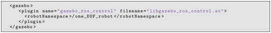
This block is an instruction to the Gazebo simulator. It brings in the plug-in library libgazebo_ros_control.so. The line

sets a namespace for the controller. controller namespace Since multiple robots may be present in the simulator, it is useful to separate their interfaces into separate namespaces. The name chosen, one_DOF_robot, must be consistent verbatim with naming in two other files: the control-parameter YAML file and the launch file (described below). control parameters
A file that must be created for use with Gazebo plug-in controllers is a controller parameter file in YAML syntax. Such files typically reside within a subdirectory for configuration files. In the the package minimal_robot_description, a subdirectory control_config was created, which contains the file one_dof_ctl_params.yaml. The contents of this file are:

Listing 3.10 one_dof_ctl_params.yaml: control gains file
The control parameter file starts with a robot name, in this case one_DOF_robot:. This name must agree with the namespace name in the gazebo tag within the URDF file.
The control parameter file associates a controller name with each controlled joint. In the present case, a controller named joint1_position_controller is associated with joint1. For additional controlled joints, this block should be replicated, assigning a unique controller name associated with each controlled joint name in the corresponding URDF file.
The type of controller specified for this example is a PID joint position controller, which is a type of servo controller with proportional, derivative and integral-error gains. The gain values are specified by the line: PID controller

which assigns values for the proportional gain (10.0 ) and the integral-error gain (10.0 ). The suggested values are not well tuned, but they are valid.
Finding good gains for joint controllers can be challenging. This can be done interactively with graphical assistance using the command:

rqt_reconfigure Use of this graphical tool for joint control parameter tuning is described at http://www.w3.org/1999/xlink.
Tuning the integral-error gain can be particularly challenging. This control gain can easily lead to instability. Using a gain of 0 is a good place to start. If this gain is non-zero, anti-windup constraints should be imposed on the integral-error computation. These are specified by the values of i_clamp_min and i_clamp_max. If integral-error feedback is not used (i.e. by setting the i: term to zero), it is not necessary to specify these values. integral-error gain
For the control parameter file to be associated with the corresponding real-time control code, the YAML file is first loaded onto the parameter server. This is conveniently done within a launch file.
A launch file that performs the necessary start-up functions for our example is minimal_robot_w_jnt_ctl.launch, contained within the minimal_robot_description package. The contents of this launch file appear in Listing 3.11.
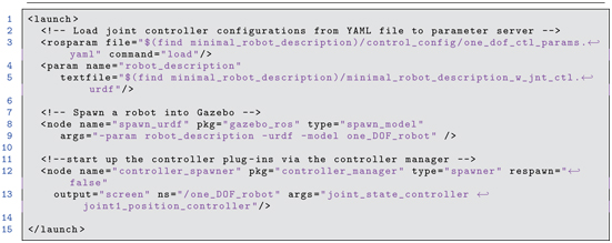
Listing 3.11 minimal_robot_w_jnt_ctl.launch: launch file for minimal robot using ROS control plug-ins
controller_spawner Line 3 of Listing 3.11 loads the control parameter file on the parameter server, where it will be accessed when the joint controllers are started. Lines 4 and 5 load the (modified) robot model URDF file onto the parameter server. Lines 8 and 9 load the robot model into the Gazebo simulator. This task was formerly done with a separate terminal command, but this operation is now automated by including it in the launch file. Also, the robot model in this instance is spawned into Gazebo by accessing it from the parameter server instead of from a file. Lines 12 and 13 use the spawner node from the controller_manager package to bring in the PID controller(s) and start them up. In this command, the argument joint1_position_controller refers to the controller name specified in the control parameter YAML file. If there are more joint controllers to be used, each controller’s name should be included in the list of arguments in this command.
Note that the controller launch command specifies ns="/one_DOF_robot". This namespace assignment must be identical to the name assigned in the control parameter YAML file as well as the namespace specified in the gazebo tag of the URDF file. namespace, robot robot namespace
A roslaunch option used in the controller launch command is: output="screen". With this option specified, roslaunch screen output printed output from the node being launched will appear within the terminal from which roslaunch is invoked. This is the case even when there are multiple nodes launched from the same launch file. (Formerly, we used rqt_console to view such messages when launching minimal_nodes, since launching multiple nodes from a single terminal suppressed their ROS_INFO displays within that terminal.)
With the preceding changes, our controlled robot can be launched as follows. First, bring up Gazebo with an empty world from a terminal with the command:

In a second terminal, launch our robot model, complete with controllers:

Terminal output from this launch ends with:
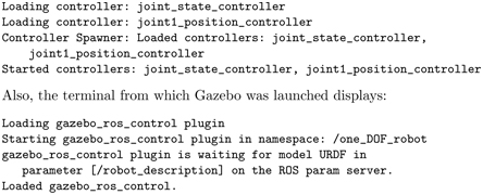
Our one-DOF robot appears in the Gazebo graphical display, identical to the initial case presented in Section 3.4. However, we now have additional topics. Running

shows the following additional topics:
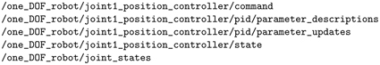
joint control topics These topics all appear under the namespace one_DOF_robot. The topic /one_DOF_robot/joint1_position_controller/command is subscribed to by Gazebo, and the message type is std_msgs/Float64. This topic is used by the joint position controller as a desired setpoint, equivalent to pos_command in our previous example minimal controller. We can use this topic to command our robot manually by entering, e.g.:

Figure 3.15 Transient response to step position command with ROS PD controller

which commands the joint to a desired angle of 1.0 rad. The resulting response is shown in Fig 3.15. The response is slow and has overshoot, calling for tuning of the control parameters. With the integral-error term active, however, the link ultimately converges virtually perfectly on the commanded setpoint of 1.0 rad.
With the preceding introductory material, we next consider a slightly more complex model in the context of a mobile robot.
3.7 Building mobile-robot model
mobile robot modeling To extend the URDF modeling introduced in Section 3.3, modeling of a simple mobile robot is presented here, introducing some additional modeling and Gazebo capabilities. An on-line tutorial for building mobile robots can be found at http://www.w3.org/1999/xlink. (See http://www.w3.org/1999/xlink for a mobile-robot modeling tutorial using SDF, which is a similar, but richer modeling format that is becoming more popular).
Extensions of URDF modeling to be introduced here include the use of xacro to help simplify URDF models, xacro and a Gazebo plug-in for inclusion of a differential-drive controller.
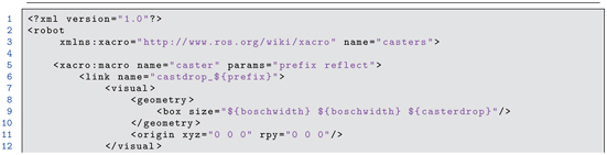
The illustrative mobile-robot model, differential-drive controller called mobot.xacro, is contained in the accompanying repository within the package mobot_urdf. The contents of mobot.xacro are given in Listing 3.12. A xacro file, xacro (see http://www.w3.org/1999/xlink), can be converted to a URDF file, but using xacro can help simplify model specification. Notably, mobot.xacro takes advantage of the xacro instruction xacro:include / to import five other xacro files. This allows distributing the modeling details over multiple smaller files with restricted contexts.
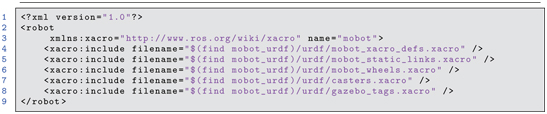
Listing 3.12 mobot.xacro: simple mobile robot xacro model file
An interpretation of the Listing 3.12 follows. Line 1, ?xml version="1.0"? , must be the first line of all xacro files. Line 3,

establishes that this file will use the xacro package for defining and using macros. Subsequent lines include five other xacro files (and these files may include other files, hierarchically).
A useful xacro capability is defining properties and macros. Examples are included in the file mobot_xacro_defs.xacro, which appears in Listing 3.13.

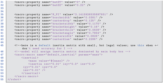
Listing 3.13 mobot_xacro_defs.xacro: xacro file that contains parameter values
Lines 6 through 43 use xacro properties to define mnemonic names to represent numerical values. This technique allows for defining URDF elements with symbolic parameters. Use of xacro properties helps to keep numerical values consistent throughout the file (which is particularly important when these values are used in multiple instances). It also makes the file easier to modify to change dimensions to tune a model to a physical system.
In addition to defining parameters, xacro allows for defining macros. For example, lines 47 through 54 define the macro default_inertial:

xacro macro This macro is used six times in the model listing, e.g. as in line 19 of casters.xacro:

Macros can be used within the definition of other macros. In fact, use of the macro default_inertial on line 19 of casters.xacro is such an instance, since it is embedded within the macro caster.
The next three files included use box and cylinder geometric objects to define the 14 links in this system, both for their visual representation and for their collision boundaries. Inertial components are defined for each link in the system. All fields within the link and joint definitions are of the same style as introduced in the minimal_robot URDF, except for the use of named parameters in place of numerical values. Details are distributed over multiple files, the first of which is mobot_static_links.xacro. This file appears in Listing 3.14.
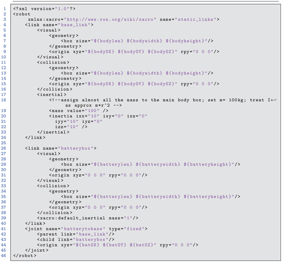
Listing 3.14 mobot_static_links.xacro: specification of static links in mobot model
The mobot_static_links.xacro file contains visual, collision and inertial properties for two links: a base_link and a batterybox. Every robot model has a root link, conventionally called base_link, that is the root of the transformation tree of all other frames of the robot. Arbitrarily many additional links (including sensor links) may be joined to the base link. The file mobot_static_links.xacro also describes a batterybox link, which is joined to the base_link through a defined fixed joint.
The third included file is mobot_wheels.xacro. This file, displayed in Listing 3.15, describes the drive wheels of the mobile robot. This description includes visual, collision and inertial properties of the wheels, along with effort and velocity limits of the named drive-wheel joints.
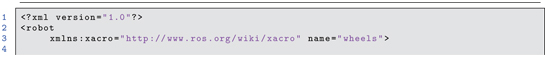

Listing 3.15 mobot_wheels.xacro: description of drive wheels
The wheel macro is used twice in the code to define symmetric left and right drive wheels through use of the prefix parameter. This allows defining links with names right_wheel and left_wheel with associated joints right_wheel_joint and left_wheel_joint. These are declared in the model file on lines 34 through 35:

Through use of this macro, it is assured that the left and right wheels will be identical, except for their placement within the model. Changes to parameter values used within this macro will still result in left and right wheels that are identical.
The file casters.xacro, which is included in mobot.xacro, contains detailed modeling of a pair of passive casters attached to the robot. Each caster has two degrees of freedom: caster swivel and caster wheel rotation. The modeling file specifies the visual, collision and inertial properties of the caster components, as well as the (passive) joint properties. This file is displayed in Listing 3.16.


Listing 3.16 casters.xacro: description of passive caster wheels
As with the drive wheels, a macro that supports creating identical, albeit reflected caster models is defined.
Finally, mobot.xacro includes the file gazebo_tags.xacro, which is shown in Listing 3.17. As with the minimal robot arm example, it is useful to include a Gazebo plug-in for joint control. For the mobot model, this is done as shown in file gazebo_tags.xacro.

Listing 3.17 gazebo_tags.xacro: gazebo block to include differential-drive plug-in
The XML code between the gazebo tags brings in the library libgazebo_ros_diff_drive.so, which is useful for differential-drive control similar to that of the previous simple two-dimensional robot simulator. To use the differential-drive libgazebo_ros_diff_drive.so plug-in, several parameters must be defined, including
- Names of the drive-wheel joints, right_wheel_joint and left_wheel_joint
- Wheel separation, track
- Name of the root of the URDF tree, which is base_link
- Topic name to be used to command speed and spin, set (per convention) to cmd_vel
Further details can be found at http://www.w3.org/1999/xlink and http://www.w3.org/1999/xlink.
To use a xacro file, one converts it to a URDF file using the xacro executable within the xacro package. For example, to convert the file mobot.xacro to a URDF with filename mobot.urdf, run the following command:

This action creates a URDF file with all of the substitutions defined by the xacro macros. The URDF file produced can be checked for consistency with the command:

which produces the output:
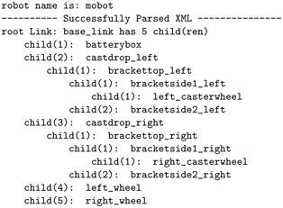
This output shows that the URDF file can be parsed logically, and it displays 14 links in the model. Relationships among the links are shown in an outline style. The tree of links also can be visualized graphically using the command:

which produces the file mobot_graphiz.pdf, which is displayed in Fig 3.16. This figure illustrates the connectivities and spatial relationships among the links. urdf_to_graphiz
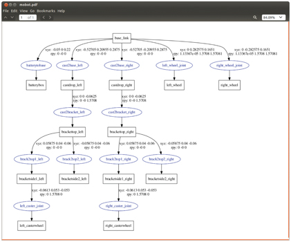
Figure 3.16 Graphical display of URDF tree for mobot
The mobot model can be loaded into Gazebo to visualize and simulate. As before, this is done by first loading the robot description file into the parameter server, then executing the spawn_model node within the gazebo_ros package, referencing the robot model on the parameter server. This is accomplished via the launch file mobot.launch in the urdf subdirectory of the package mobot_urdf. First, Gazebo is started with the command:

Then the mobot model is inserted into the Gazebo simulation by running the corresponding launch file:

The resulting Gazebo display is shown in Fig 3.17. The Gazebo option view->joints has been enabled. Note that we can see 6 movable joints: two joints corresponding to the two large drive wheels, and four joints associated with the passive casters. Gazebo, view joints
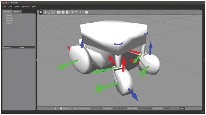
Figure 3.17 Gazebo view of mobot in empty world
3.8 Simulating mobile-robot model
As noted earlier, the robot model can be introduced in the Gazebo simulator by

after which the mobot model is inserted into the Gazebo simulation by running the corresponding launch file:

At this point, the mobile robot can be controlled via the cmd_vel topic, identical to what was done with the simple two-dimensional robot simulator. For example, the command:

causes the robot to move in a counter-clockwise circle.
We can also command the robot under program control, as formerly illustrated with the STDR simulator, or with a teleoperation program. Use of such command nodes with different robots is made simpler through a ROS feature of topic remapping. remapping topic remapping This can be seen by re-using the stdr_open_loop_commander node from the package stdr_control introduced in Section 3.1. Note that the stdr_open_loop_commander.cpp code publishes to the topic /robot0/cmd_vel, whereas our differential-drive controller of the mobot model expects commands on topic cmd_vel. We can re-use the stdr_open_loop_commander node nonetheless if we remap the output topic name. From the command line, this can be invoked by entering:

By using the option /robot0/cmd_vel:=cmd_vel, when this command is executed, the output from stdr_open_loop_commander is redirected from /robot0/cmd_vel to cmd_vel, and our mobot responds.
Topic remapping can also be performed within launch files, as illustrated in open_loop_squarewave_commander.launch within the launch subdirectory of package mobot_urdf.
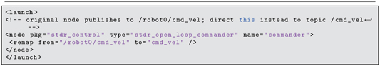
Listing 3.18 open_loop_squarewave_commander.launch
Running this launch file has the same effect as the previous command line execution with topic remapping.
An alternative, more convenient means to send Twist commands to the robot interactively is by running a keyboard teleoperation node, e.g.:

teleop_twist_keyboard (This package should be installed by the provided installation scripts, or it can be installed manually. See http://www.w3.org/1999/xlink.) This node takes keyboard input to command linear and angular velocities, and these commands are published as a Twist message to the cmd_vel topic, resulting in robot motion. This interface works as well with the STDR simulator or with any mobile robot that subscribes to a velocity-command interface with a Twist message type (which is the de facto standard in ROS). By default, this node publishes Twist commands to the topic cmd_vel, although this can be remapped (e.g. to control the STDR simulator). Twist command
An important difference of the URDF model in Gazebo versus the STDR simulator is that the Gazebo simulation includes physics. Inertias, friction, controller dynamics and actuator saturation are taken into account. With the Gazebo simulation of the mobot running, invoking the launch file:

commands the robot to move, and the resulting response can be plotted with rqt_plot. The mobot simulation in Gazebo publishes its state to the odom topic, from which we can plot the robot forward velocity in response to step velocity commands. As seen in Fig 3.18, the robot does not change velocities instantaneously.
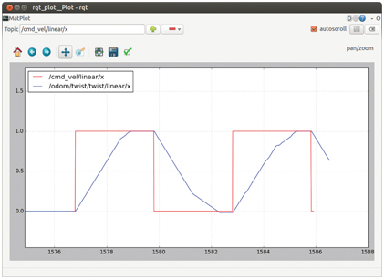
Figure 3.18 Response of mobot to step velocity commands in Gazebo simulation
One of the idiosyncrasies of the default physics simulator, open dynamics engine, is that it does not do a good job of modeling sustained stiff contact ODE, stiff contact stiff contact between separate models. This is noticeable with wheels or feet on the ground, as well as gripper fingers grasping objects. This can be observed with the simple mobile robot model. After starting Gazebo and inserting the mobot model, the robot will slowly slip to its left. Actually, the robot wheels are chattering against the ground. This can be seen in the Gazebo viewer by enabling view->contacts from the top menu bar. An example screenshot with contacts displayed appears in Fig 3.19. The blue markers are points of contact and the green lines show the direction and (by length) the magnitude of the contact forces. At this instant, the contact forces on wheels are stronger on its left side than on its right. However, if the display is viewed dynamically, the contact forces can be seen to toggle on and off and to shift around due to numerical instability of modeling stiff contact. This problem is exacerbated by the fact that the robot has four wheels, and simultaneous contact of four points with a flat plane is numerically challenging. As a result, the robot seems to constantly vibrate on the ground.
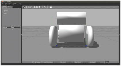
Figure 3.19 Gazebo simulation of mobot with contacts display enabled
A few adjustments can be made to try to improve the numerical stability. Within the URDF (or xacro file), insert the lines:
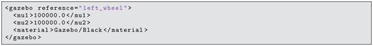
Gazebo model friction and repeat the block for right_wheel as well. This Gazebo tag passes parameters to the physics engine, declaring a custom friction property. In fact, the mu coefficients are not realistically physical. They do influence the simulation, but these values cannot be treated like genuine dimensionless Coulomb friction components. Some experimentation may be required to achieve acceptable simulation results for sustained contact simulations, including wheels, feet and fingers.
The line material Gazebo/Black /material gazebo delimiters. The result of the example insertion (repeated for left and right wheels) is that the model appears with black wheels. Gazebo material colors
Another variation that can be introduced is to tell the simulator to run more iterations of internal computations each time step (where the time step is, by default, 1 ms). This can result in better fidelity of simulation, including Gazebo time step Gazebo numerical iterations less chatter with sustained, stiff contacts. But this is done at the price of more demanding computation, potentially resulting in a lower real-time factor. The iterations parameter can be changed with a Gazebo tag in the URDF or interactively from the Gazebo window. For the latter, on the left pane, choose the World tab, then under physics->solver->iterations, edit the numerical value from its default value (50) to something larger (e.g. 200). This change can slow the side slip of the mobot model to be imperceptible.
The mobile-robot simulation can be made more interesting by introducing elements in the world model. This can be done by manually inserting existing models or by inserting custom-designed models. An interesting world model that can be inserted from the Gazebo Insert tab is Starting Pen. After selecting this model from the Insert tab, the user has the opportunity to move the corresponding model around in the simulated world to a desired location (via the mouse), then click to complete the model placement. Figure 3.20 shows the mobot model within a virtual world that includes the starting pen model.
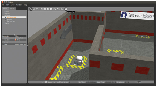
Figure 3.20 Gazebo display of a mobot in starting pen
3.9 Combining robot models
Since robot URDF files can get quite long, it is useful to be able to include subsystems within a single model file. Similarly, it is convenient to include launch files within launch files. URDF, combining models
To illustrate, we will mount our minimal robot arm model onto our simple mobile base. Revisiting the minimal arm model in the minimal_robot_description package, we make a simple change to the URDF to create the file minimal_robot_description_unglued.urdf. Importantly, we delete the joint glue_robot_to_world, so our arm can be attached to the mobile base instead. To make the arm more attractive, the following material tags are added to colorize the links:

We can combine the mobile-platform and minimal arm models as illustrated by the file mobot_w_arm.xacro, the contents of which are shown in Listing 3.19.

Listing 3.19 mobot_w_arm.xacro: model file combining mobot and minimal arm
The xacro file of Listing 3.19 resides in the mobot_urdf package. Lines 4 and 5:

use the include feature of xacro to bring in two files verbatim. The named file paths start with . This syntax informs the launcher to search for the named files by stated package name (mobot_urdf in this example). Specifying directories in this manner simplifies specifying the search path, and it also makes the launcher more robust. Packages installed in a different system under different directories can still be found using this syntax.
After bringing in both the mobile base and the simple arm models, the arm is attached to the base by declaring a new (fixed) joint, arm_base_joint:
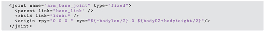
This new joint specifies how link1 (the first link of the arm model) is to be attached to its parent, base_link (the base link of the mobile-platform model). The arm model is offset in y and z, using xacro parameters, to center the base of link1 on the top of the main link of the mobile robot. joint, fixed
In addition to combining URDF (or xacro) models, it is also convenient to combine launch files. Our launch file for the robot arm, minimal_robot_w_jnt_ctl.launch, performed three functions: it loaded the arm URDF onto the parameter server, it spawned the robot model from the parameter server into Gazebo, and it started the ROS joint position controller(s). Since our integrated mobile base with arm is a new model, we wish to separate the arm-specific launch commands from the model loading and spawning. For this purpose, a smaller launch file in the minimal_robot_description package, called minimal_robot_ctl.launch, is created. The contents of this file appear in Listing 3.20.

Listing 3.20 minimal_robot_ctl.launch: launch file for starting arm controller
A launch file for the integrated robot model resides in the mobot_urdf package within the launch subdirectory, named mobot_w_arm.launch. The contents of this launch file appear in Listing 3.21.

Listing 3.21 launch file combining mobot and minimal arm
launchfile, including files This launch file loads the combined xacro file onto the parameter server and spawns this model into Gazebo. The line:

searches for the file minimal_robot_ctl.launch in the minimal_robot_description package and includes this launch file verbatim.
After launching Gazebo, the integrated launch file can be invoked with:

The resulting Gazebo display appears in Fig 3.21.
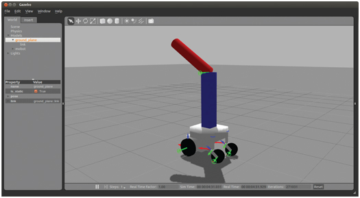
Figure 3.21 Gazebo display of combined mobile base and minimal arm models
Running:

shows that the following topics are active:
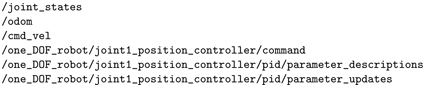
We thus see that command interface topics are available for both the mobile platform and the arm. Feedback values of joint states for both the arm and mobile base are available as well.
3.10 Wrap-Up
Our robot modeling so far has been quite crude in utilizing only primitive boxes and cylinders. Nonetheless, we have seen the basic elements of modeling, including kinematic, dynamic, visual and collision properties, as well as use of plug-ins for physically realistic controllers. The simple examples illustrate modeling both of articulated mechanisms and mobile vehicles.
Making more sophisticated models involves extending the same techniques to more joints and using CAD-file descriptions that offer more detailed and realistic modeling of visual and collision properties. A few examples examples of more realistic robot models are shown in Figs 3.22 through 3.24.
The Baxter [9] robot model in Fig 3.22 includes control over 15 joints (7 per arm plus a neck pan motion) plus grippers (which can be substituted). Sensor outputs include the dynamic state of every joint, streaming images from three color cameras, distance sensors from the wrists, and sonar sensors around the head. This model is realistic in terms of its kinematics (including joint limits), actuator behavior (including torque saturations), visual appearance and collision characteristics. The robot is highly dexterous and well instrumented. Further, the model is publicly available [37]. Consequently, this model will be used in this text for further examples in use of ROS for sensing and manipulation.

Figure 3.22 Gazebo display of Baxter robot model
The model in Fig 3.23 is of a dual-arm DaVinci surgical robot [41]. The CAD descriptions have been posted by Johns Hopkins University [16,18]. Inertial parameters and ROS controller plug-ins were added to make this model Gazebo compliant. The resulting system is useful for testing extensions to computer-assisted robotic surgery and potentially development of a surgical training system.

Figure 3.23 Gazebo display of DaVinci robot model
Figure 3.24 shows the Boston-Dynamics, Inc. Atlas robot [6]; the model was developed by the Open Source Robotics Foundation (OSRF) [1] for the DARPA 1 Robotics Challenge [30]. This model was used by teams to develop code for the DARPA competition tasks, including both bipedal motion control and object manipulations (e.g. valve turning). Given the risk, difficulty and crew size required to perform physical experiments with Atlas, this model helped teams develop code more quickly, enabling individuals to make progress in parallel and to perform extensive software debugging and testing in simulation before moving to physical trials.

Figure 3.24 Gazebo display of Atlas robot model
It should be appreciated that robot models in Gazebo include realistic physical interactions, including collisions, effects of gravity and inertial effects. Simulators that lack these properties can be used to evaluate viability of kinematic trajectories in terms of reachability, but simulators that lack physics engines cannot evaluate dynamic effects, including walking or object manipulation.
An even stronger motivation for using a physics-based simulator is incorporation of sensor simulation. Gazebo is capable of simulating physical sensors acting in a virtual environment. Plug-ins for sensors include color cameras, LIDARs, depth cameras (including the Microsoft Kinect [38]), stereo cameras, accelerometers, force sensors, and sonar sensors. With emulation of sensors, one can develop sensor-based behaviors that are testable in Gazebo. Since such development can be time consuming, having a suitable simulator is a valuable productivity tool.
Integrating sensory data requires reconciling all model and sensor information to a common reference frame, which requires extensive use of coordinate transforms in ROS, which is introduced next.
1 DARPA: Defense Advanced Research Projects Agency of the U.S. Department of Defense.