CHAPTER 6
Using Cameras in ROS
CONTENTS
6.1 Projective transformation into camera coordinates
6.2 Intrinsic camera calibration
6.3 Intrinsic calibration of stereo cameras
6.4.1 Example OpenCV: finding colored pixels
6.4.2 Example OpenCV: finding edges
INTRODUCTION
Cameras are commonly used with robots. To interpret camera data for purposes of navigation or grasp planning, one needs to interpret patterns of pixel values (intensities and/or colors) and associate labels and coordinates with these interpretations. This chapter will introduce conventions for camera coordinate frames in ROS, camera calibration, and low-level image-processing operations with OpenCV. Extensions to 3-D imaging are deferred to Chapter 7. camera calibration
6.1 Projective transformation into camera coordinates
A necessary step toward projective transformation associating images with spatial coordinates is camera calibration. This includes intrinsic properties and extrinsic properties. camera model, intrinsic parameters The intrinsic properties of a camera remain constant independent of the way the camera is mounted or how it moves in space. Intrinsic properties include image sensor dimensions (numbers of rows and columns of pixels); the central pixel of the image plane (which depends on how the image plane is mounted relative to the idealized focal point); distance from the image plane to the focal point; and coefficients of a model of lens distortion. Extrinsic properties describe how the camera is mounted, which is specified as a transform between a frame associated with the camera and a frame of interest in the world (e.g. the robot’s base frame). The camera’s intrinsic properties should be identified before attempting to calibrate the extrinsic properties.
Calibrating a camera requires defining coordinate frames associated with the camera. An illustration of the standard coordinate system of a camera is shown in Fig 6.1.
The point “C” in Fig 6.1 corresponds to the focal point of a pinhole camera model (i.e., “C” is the location of the pinhole). This point is referred to as the projection center, and it will constitute the origin of our camera frame. projection center camera model, projection center
The camera will have a sensor plane (typically, a CCD array) behind the focal point (between the sensor plane and objects in the environment viewed by the sensor). This sensor plane has a surface-normal direction vector. We can define the optical axis as the unique camera model, optical axis vector perpendicular to the sensor plane passing through point “C.” The optical axis defines the z axis of our camera coordinate frame. The sensor plane will also have rows and columns of pixels. We define the camera frame x axis as parallel to sensor rows, and the y axis as parallel to sensor columns, consistent with a right-hand frame (X,Y,Z). Choice of positive direction of X depends on how the sensor defines increasing pixel column numbers. camera frame
The projection of light rays from the environment to the sensor plane results in inverted images. It is mathematically convenient to avoid consideration of image inversion by assuming a virtual image plane that lies in front of the focal point (between the focal point and objects viewed). This image plane, or principal plane, is defined parallel to the camera model, principal plane physical sensor device, but offset by distance “f” (the focal length) in front of the projection center. camera model, focal length This principal plane has two local coordinate system: (x, y) and (u, v). The directions of the x and u axes are parallel, as are the directions of the y and v axes. The origin of the (u, v) frame is one corner of the image plane, whereas the origin of the (x, y) frame is near the center of the principal plane. To be precise, the origin of the (x, y) system is at point “c” in Fig 6.1, which corresponds to the intersection of the optical axis with the principal plane. Additionally, the frames (x, y) and (u, v) have different units. The (x, y) dimensions are metric, whereas the (u, v) coordinates are measured in pixels. The u coordinate ranges from 0 to NCOLS-1, where NCOLS is the number of columns in the sensor; v ranges from 0 to NROWS-1, where NROWS is the number of rows. (A common sensor dimension is = NCOLS NROWS). Data from the camera will be available in terms of light intensities indexed by (u, v) (in each of three planes, for color cameras).
The location of point “c” ideally is near u = NCOLS/2 and v = NROWS/2. In practice, the actual location of point “c” on the principal plane will depend on assembly tolerances. The true coordinates of point “c” are , which defines a central pixel known as the optical center. optical center camera model, optical center The coordinates of the central pixel are two of the intrinsic parameters to be determined.
Conversion from (x, y) coordinates to (u, v) coordinates requires knowledge of the physical dimensions of the pixel sensor elements in the detector. These elements, in general, are not square. Conversion from (x, y) to (u, v) can be expressed as: and , where is the width of a pixel and is the height of a pixel.

Figure 6.1 Standard camera frame definition.
In Fig 6.1, a point “M” in the environment is shown, where light emanating from this point (presumably background light reflecting off the object) is received by our detector. Following a ray from point “M”, passing through the focal point (the projection center) results in intersection with our principal plane at image point “m”. Point M in the environment has coordinates M(X, Y, Z), as measured with respect to our defined camera frame. The projected image point “m” has coordinates m(x, y) in the principal-frame coordinate system. If the coordinates of M are known with respect to the camera frame, the coordinates of m can be computed as a projection. Given the focal length “f”, projection may be computed as and (where x, f, X, Y and Z are all in consistent units, e.g. meters). Additionally, with knowledge of the optical center in pixel coordinates and knowledge of the pixel dimensions and we can compute the coordinates (u, v) of the projection of this optical ray onto our sensor. This projection computation thus requires knowledge of five parameters: f, , , and . This set of parameters can be further reduced by defining and , where and are treated as separate focal lengths measured in units of pixels. Using only four parameters, , , , and , it is possible to compute projection from the environment onto (u, v) coordinates in the principal plane. These four parameters are intrinsic, since they do not change as the camera moves in space. Identifying these parameters is the first step in camera calibration.
Beyond a linear camera model, one can also account for lens distortion. Commonly, this is done by finding parameters for an analytic approximation of radial and tangential distortion as follows. Given M(X, Y, Z), one can compute the projection m(x, y). The values of (x, y) can be normalized by the focal length: . In these dimensionless units, distortion can be modeled to map linear projection onto projection subject to distortion, and the resulting prediction of light impingement can then be converted to (u, v) pixel coordinates. A distortion model to map onto is (see http://www.w3.org/1999/xlink): camera model, distortion
1
2
where . Note that when all coefficients are zero, the distortion formula degenerates to simply and . Also, for pixels close to the optical center “c”, the (dimensionless) value of r will be small, and thus the higher order terms in Equations 1 and 2 will be negligible. The distortion model often includes and disregards higher order terms. Discovery of distortion model coefficients is also part of the intrinsic parameter calibration process, which will be described next.
6.2 Intrinsic camera calibration
intrisic camera calibration ROS provides support for intrinsic camera calibration through the cameracalibration package (which camera_calibration package consists of a ROS wrapper on camera calibration code originating from openCV). Theory and details of the process can be found in the OpenCV documentation (see http://www.w3.org/1999/xlink).
The calibration routine assumes use of a checkerboard-like vision target with known numbers of rows and columns and known dimensions. Calibration can be as simple as waving the calibration target in front of the camera while running the calibration process. The process will acquire snapshots of the target, inform the user when there are a sufficient number of good images for identification, then compute the intrinsic parameters from the acquired images.
This process can be illustrated in simulation, given a Gazebo emulation of a camera, a model for the vision target, and means to move the vision target in front of the camera.
Emulation of cameras in Gazebo was introduced in Section . In the simplecameramodel package (in Part 3 of the associated repository), emulation of a camera in Gazebo is specified with only a static robot acting as a camera holder. The xacro file appears in Listing 6.3.
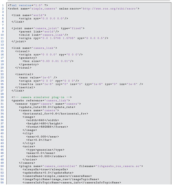
Listing 6.1 simple_camera_model.xacro: simple camera model
This model file specifies a camera located 0.5 m above the ground plane, oriented facing downward (looking at the ground plane). The model camera has pixels and publishes images encoded with eight bits each for the red, green and blue channels. Noise can be modeled, but it has been set to zero in this simple model. Radial and tangential distortion coefficients can be specified in the model as well; in the present case, these have been set to zero to emulate an ideal (linear) camera. The focal length is specified indirectly by specifying a field-of-view angle of 0.6 rad. Emulated images will be published to the topic /simplecamera/imageraw.
Our robot can be launched into Gazebo with the command:

This command invokes the simplecamerasimuwcheckerboard.launch file within the launch subdirectory of the package simplecameramodel. This launch file performs multiple steps, including starting Gazebo, setting gravity to 0, loading the simple camera model onto the parameter server and spawning it into Gazebo, and finding and loading a model called smallcheckerboard. camera calibration template
With Gazebo running and the camera model spawned, rostopic list shows 13 topics under /simplecamera. camera topics Running:

shows that images are published at 30 Hz, which is consistent with the update rate specified in the Gazebo model. Running:

shows that the message type on this topic is sensormsgs/Image. Running:

shows that this message type includes a header, specification of imager dimensions (height and width in pixels is , in this case), a string that describes how the image is encoded (rgb8, in this case), a step parameter (number of bytes per row, which is 1920 = 3 640, in this case) and a single vector of unsigned 8-bit integers comprising the encoded image.
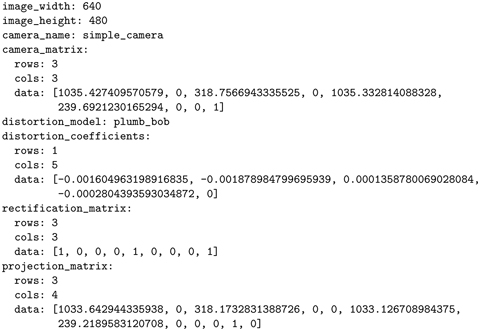
Another topic of interest is /simplecamera/camerainfo. This topic carries messages of type sensormsgs/CameraInfo, which contains intrinisic camera information, including number of rows and columns sensor_msgs/CameraInfo of pixels, coefficients of the distortion model, and a projection matrix that contains values of , , , and . Running:


This camera data includes the width and height of the sensor ( ), distortion coefficients that are all zero, and a projection matrix that sets (focal length, in pixels, for a sensor with square pixels). The focal length and horizontal width are consistent with the specified horizontal field of view (set to 0.6 rad in the model). This can be confirmed by:
3
The projection matrix, P, also specifies , which is close to half the width and projection matrix camera projection matrix half the height of the image array. (It is surprising that these values are not (319.5, 239.5), and this is possibly a Gazebo plug-in error.) The camera_info values reported on topic /simplecamera/camerainfo are consistent with the model specifications for our emulated camera. Although these values are known (by construction), one can nonetheless perform virtual calibration of the camera emulating the same procedure used with physical cameras. The vision target used for this calibration is a model of a checkerboard.
The smallcheckerboard model is located in package exmplmodels under subdirectory smallcheckerboard. The checkerboard model consists of seven rows and eight columns of 1 cm squares, alternating black and white. These squares create six rows and seven columns of internal four-corner intersections, which are used as precise reference points in the calibration process. After launching simplecamerasimuwcheckerboard.launch, the emulated camera images can be viewed by running:

The node imageview from the imageview package subscribes to image messages on the topic image and displays received images in its own display window. To get this node to subscribe to our images on topic /simplecamera/imageraw, the image topic is re-mapped on the command line with the option image:=/simplecamera/imageraw.
With these processes running, the screen appears as in Fig 6.2.

Figure 6.2 Gazebo simulation of simple camera and display with image viewer.
This figure shows the crude rectangular prism representing the camera body, with optical axis pointing down towards the ground plane. The checkerboard is hovering 0.2 m above the ground plane, approximately centered in the camera’s field of view. A light source in the Gazebo simulation casts shadows of both the camera body and the checkerboard onto the ground plane. The display from imageview shows that the camera sees the checkerboard, approximately centered in the camera’s field of view. Part of the shadow cast by the checkerboard is also visible in the synthetic image computed for the virtual camera.
To simulate waiving the vision target (checkerboard) in front of (below) the camera, a node is used to command Gazebo to move this model. Moving the checkerboard uses the same Gazebo interface introduced in Section . The code for moving the checkerboard is in the src directory of the examplecameracalibration package, source file name movecalibrationcheckerboard.cpp. This routine generates random poses for the checkerboard, approximately constrained to remain within the camera’s field of view. The checkerboard is moved vertically, horizontally, and tilted at arbitrary skew angles. The checkerboard poses are held for 0.5 sec each. Random motion generation of the checkerboard is initiated with:

The ROS camera-calibration tool can then be launched with:

This brings up an interactive display, as shown in Fig 6.3. The options to the camera calibrator node specify that there should be internal corners in the image target, that each square of the target is 1 cm 1 cm, that the image topic to which our camera publishes is /simplecamera/imageraw, and that the name of our camera is simplecamera.
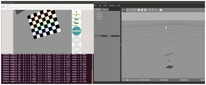
Figure 6.3 Camera calibration tool interacting with Gazebo model.
As this routine runs, it acquires snapshots of the vision target at different poses. It applies image processing to each such snapshot to identify the 42 internal corners. It displays acquired images with a graphical overlay illustrating identification of the internal corners (as seen in the colored lines and circles). As the calibration node runs, it continues to acquire sample data and informs the operator of the status of its calibration set. The horizontal bars under X, Y, size and skew in the calibration viewer indicate the range of contributions of vision target samples. When these bars are all green (as in Fig 6.3), the calibrator is suggesting that the data acquired so far is sufficient to perform calibration. When this is the case, the circle labeled “calibrate” changes from gray to green, making it an active control. Once this is enabled, the operator can click on this button to initiate parameter identification. A search algorithm is then invoked to attempt to explain all of the acquired data (with associated internal corner points) in terms of intrinsic camera coordinates. (As a by-product, the algorithm also computes an extrinsic pose estimate for each of the template snapshot poses.) Once the identification algorithm has converged, calibration results will be displayed and the Save and Commit buttons will be enabled.
Clicking Save and then clicking Commit results in camera parameters written to the directory .ros (a hidden directory under your home directory). Within the .ros directory, a subdirectory called camerainfo will be created, which will contain a new camera_info directory file called simplecamera.yaml. For an example calibration process as above, the output yaml file contains the following: camera calibration YAML file contains the following:
At this point, running rostopic echo /simplecamera/camerainfo shows that the new camera parameters are being published. The camera still has identically pixels (as it must), but there are now non-zero (though small) distortion parameters. These values are actually incorrect (since the simulated camera had zero distortion). However, these are the values found by the calibration algorithm. This shows that the calibration algorithm is only approximate. Better values might be obtained with more images acquired before initiating the parameter search.
Similarly, the values of , , and are slightly off. The focal-length values indicate nearly square pixels (1033.64 versus 1033.13), and these are close to the true model value (1034.47). The central coordinates of are close to the model values of (320.5, 240.5). These values, too, might be improved by acquiring and processing more calibration data.
This concludes the description of how to use the ROS camera calibration tool, and it provides some insight into the meaning of the camera parameters and expectations of the precision to which one can expect calibration to be achieved.
As noted earlier, calibration of a single camera is insufficient in itself to derive 3-D data from images. One must augment this information with additional assumptions or with additional sensors to infer 3-D coordinates from image data. Stereo vision is a common means to accomplish this. Calibration of a stereo vision system is described next.
6.3 Intrinsic calibration of stereo cameras
stereo camera calibration Stereo cameras offer the opportunity to infer 3-D from multiple images. A prerequisite is that the stereo cameras are calibrated. Commonly, stereo cameras will be mounted such that the transform between their respective optical frames is constant (i.e. a static transform). In this common situation, the coordinate transform from the left optical frame to the right optical frame is considered intrinsic, since this relationship should not change as the dual-camera system is moved in space. For efficiency of stereo processing, this transform is described in terms of two rectification matrices and a single baseline dimension. These components must be identified in addition to the monocular-camera intrinsic parameters for each of the cameras.
The simple camera model is extended to dual (stereo) cameras in the model file multicameramodel.xacro in package simplecameramodel. This model file includes two cameras, both at elevation 0.5 m. To assist with visualization, this model file specifies that the left camera body will be colored red in Gazebo. (Specification of colors in rviz, unfortunately, is not consistent with color specifications in Gazebo.) In this model, the left camera has its optical axis pointing anti-parallel to (and colinear with) the world z axis, and the image-plane x axis is oriented parallel to the world y axis. The right camera is offset by 0.02 m relative to the left camera. This offset is along the positive world y axis, which is also 0.02 m along the left-camera image-plane positive x axis. These frames are illustrated in Fig 6.4, which shows the left-camera optical frame, the world frame, and the locations of the left and right camera bodies.

Figure 6.4 Rviz view of world frame and left-camera optical frame in simple stereo camera model.
The model file includes the Gazebo elements shown below:


The camera specifications, right and left, are identical to the specifications used in the prior simple camera model, with zero distortion, zero noise, pixels, and 0.6 rad horizontal field of view. Importantly, instead of specifying:

the stereo model specifies:

The reference frame for this system is the leftcameraoptical_frame. A 0.02 m baseline is specified, meaning that the right camera is offset from the left camera by a distance of 0.02 m along the positive x axis of the left camera optical frame. 1
The stereo camera model can be launched with:

Note that this launch file also starts the robotstatepublisher node, which publishes the model transforms, and thus enables rviz to display frames of interest.
With this model running in Gazebo, there are twice as many camera topics (for left and right cameras). Running: displays (in part):
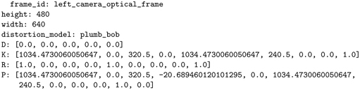
As with the monocular camera, the focal length (in pixels) is 1034.47, and . The K matrix and the R matrix are identical for the left and right cameras, and these are identical to the previous monocular camera example. The only difference is that the projection matrix (P matrix) of the right camera has a translation term (first row, third column) that is non-zero (specifically, ). This translation component is , where b is the baseline displacement of the right camera with respect to the left camera.
Performing stereo camera calibration incorporates the elements of monocular camera calibration to identify the intrinsic camera properties. In addition, stereo calibration finds rectification transforms for the two cameras. The intent of rectification is to transform the left and right images into corresponding virtual cameras that are perfectly aligned, i.e. with image planes that are coplanar, optical axes that are parallel, and x axes that are parallel and colinear. rectification, stereo cameras stereo camera rectification Under these conditions, the following highly useful property is obtained: for any point M in the environment that projects onto the left and right (virtual) image planes, the corresponding left and right y values (and v values) of the projected points will be identical in the left and right images. This property dramatically simplifies addressing the correspondence problem, in which one needs to identify which pixels in the left image correspond to which pixels in the right image, which is a requirement for inferring 3-D coordinates via triangulation.
To perform stereo camera calibration, the ROS node cameracalibrator.py can again be used, but with more cameracalibrator.py node parameters specified. This process is detailed on-line at http://www.w3.org/1999/xlink and illustrated at http://www.w3.org/1999/xlink. For our simulated stereo cameras, we can again use the model checkerboard and random pose generation, as follows. First, launch the multi-camera simulation:

Next, insert the checkerboard template with the command:
roslaunch simple_camera_model add_checkerboard.launch
Move the checkerboard in Gazebo to (constrained) random poses with:

The calibration tool can be started with:

In this case, there are quite a few additional options and specifications. The checkerboard is again described as having internal intersections among 0.010 m squares. The image topics right and left are remapped to match the topic names corresponding to the right and left cameras of our simulated system. The option fix-aspect-ratio enforces that the left and right cameras must have , which enforces that the pixels are square. This constraint reduces the number of unknowns in the parameter search, which can improve the results (if it is known that the pixels are, in fact, square). The option zero-tangent-dist enforces stereo camera calibration, fix-aspect-ratio stereo camera calibration, zero-tangent-dist stereo camera calibration, fix-principal point that the camera model must assume zero tangential distortion, i.e. that the and coefficients are coerced to be identically zero; this removes these degrees of freedom from the calibration parameter search. The option fix-principal-point coerces the values of to be in the middle of the image plane (which is true for our simple camera model, but not generally in practice). With these simplifications, the calibration process (parameter optimization) is faster and more reliable (provided the assumptions imposed are valid).
Figure 6.5 shows a screenshot during the calibration process. The camera bodies are rendered in Gazebo side by side and facing down, viewing the movable checkerboard. The graphical display for the calibration tool shows the left and right images, as well as the identification of internal corners on both images. As with monocular calibration, the graphical display shows when the data acquisition is determined adequate to perform valid calibration.

Figure 6.5 Screenshot during stereo camera calibration process, using simulated cameras.
Once data acquisition is sufficient for calibration, the calibrate button changes from to green. Clicking on this button initiates the algorithmic search for optimal calibration parameters. This can take several minutes (although it is much faster with the parameter-constraints imposed in this example). After completion, the save and commit buttons are enabled, and clicking these will store the resulting calibration in /.ros/camerainfo/stereocamera in files left.yaml and right.yaml. stereo camera calibration file Results for an example calibration are:
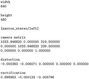

Rectification for the left camera is essentially a identity matrix, meaning this camera is already virtually perfectly aligned in the epipolar frame. The epipolar frame right-camera rectification rotation matrix is also essentially the identity, since the Gazebo model specified the right camera to be parallel to the left camera (and thus no rotation correction is necessary). camera matrix The camera matrix contains intrinsic parameters of each camera. Note that, for both cameras, , which is the middle of the sensor plane (as mandated by the option fix-principal-point). Also, for both left and right cameras, which was enforced as an option. However, for the left camera, and for the right camera. These should have been identical at . This shows that the calibration algorithm (which performs a non-linear search in parameter space) is not perfect (although the identified values may well be adequately precise).
The left-camera projection matrix has a fourth column of all zeros. The right-camera projection matrix has . This value is close to the ideal model value of .
In the present (simulated) case, the camera calibration parameters are, in fact, known identically, since these are specified in the Gazebo model. When the Gazebo simulation is restarted, the simulated cameras will use the model-specified parameters. More generally, calibration of physical cameras is a necessary step. After performing calibration (e.g. using the described checkerboard method), the identified calibration parameters will be stored in the .ros directory, and when the camera drivers are subsequently launched, these stored calibration values will be read from disk and published on the corresponding camerainfo topic.
An alternative to the multicamera plug-in is the model stereocam.xacro in package simplecameramodel. In this model file, two individual cameras are defined, where each camera is specified as in our monocular-camera example. This alternative model can be launched with:

This will result in separate camera publications (left and right). This model file has more intuitive frame specifications than the multicamera plug-in. A complication of modeling separate cameras, however, is that the image publications will have different time stamps. In performing stereo-vision analysis, right and left images must have adequate temporal correspondence to interpret dynamic data. That is, if the cameras are moving or if objects in the environment are moving, triangulation is only valid when operating on left and right images that are acquired synchronously. (For static scenes with static cameras, synchronization is not a concern.) stereo camera frame synchronization
Defining separate camera drivers in the model file results in asynchronous image publications. As a result, the camera-calibration node and subsequent stereo image processing node will not accept the asynchronous images. If it is known that the image analysis will be performed with stationary cameras viewing stationary objects (e.g. interpreting objects on a table after a robot has approached the area), it is justifiable to modify the image topics to spoof synchronism. This can be done, for example, by running:

This node simply subscribes to the raw left and right image topics, /unsynced/left/image_raw and /unsynced/right/image_raw, re-assigns the time stamp in the respective message headers as:

then re-publishes the images on new topics, /stereo_sync/left/image_raw and /stereo_sync/right/image_raw. The input and output topics can be re-mapped at run time to match the topic names of the actual cameras and the desired topic names for subsequent processing. With the stereo_sync node running, pairs of recently received left and right images will produce output image topics with identical time stamps. This will enable use of stereo calibration and stereo processing nodes.
6.4 Using OpenCV with ROS
OpenCV (see http://www.w3.org/1999/xlink)is an open-source library of computer vision functions. It was initiated by Intel in 1999, and it has become a world-wide popular resource for computer vision programming. To leverage the capabilities of OpenCV, ROS includes bridge capabilities to translate between ROS-style messages and OpenCV-style objects (see http://www.w3.org/1999/xlink). OpenCV
In addition to accommodating OpenCV classes, ROS also has customized publish and subscribe functions for working with images. The imagetransport framework in ROS comprises both classes and nodes for managing transmission of images (see http://www.w3.org/1999/xlink). Since images can be very taxing on image_transport communications bandwidth, it is important to limit network burden as much as possible. There are publish and subscribe classes within imagetransport that are used essentially identical to ROS-library publish and subscribe equivalents. The behaviors of the imagetransport versions are different in a couple of ways. First, if there are no active subscribers to an imagetransport publisher, images on this topic will not be published. This automatically saves bandwidth by declining to publish large messages that are not used. Second, imagetransport publishers and subscribers can automatically perform compression and decompression (in various formats) to limit bandwidth consumption. Invoking such compression merely requires subscribing to the corresponding published topic for the chosen type of compression, thus making this process very simple for the user.
In this section, simple use of OpenCV with ROS is illustrated. This information is not intended to be a substitute for learning OpenCV; it is merely a demonstration of how OpenCV can be used with ROS.
6.4.1 Example OpenCV: finding colored pixels
The file findredpixels.cpp in the package exampleopencv of the accompanying repository attempts to find red pixels in an image. The package exampleopencv was created using:

In this package, imagetransport is used to take advantage of the efficient publish and subscribe functions customized for images. The cvbridge library enables conversions between OpenCV datatypes and ROS messages. The sensormsgs package describes the format of images published on ROS topics.
The CMakeLists.txt file auto-generated using cscreate_pkg contains a comment describing how to enable linking with OpenCV:

By uncommenting findpackage(OpenCV REQUIRED) (as above), your source code compilation within this package will be linked with the OpenCV2 library (which is the supported version for ROS Indigo and Jade). OpenCV and CMakeLists.txt CMakeLists.txt and OpenCV
The example source code findredpixels.cpp (in the /src sub-directory) computes two output images. One of these is a black and white image for which all pixels are black except for the locations of pixels in the input image that are considered to be sufficiently red (and these pixels are set to white in the output image). The second output image is a copy of the color input image, but with superimposed graphics corresponding to a small blue block displayed at the centroid of the red pixels. The code is shown in Listings 6.2 through 6.4.

Listing 6.2 find_red_pixels.cpp: C++ code to find centroid of red pixels, class definition
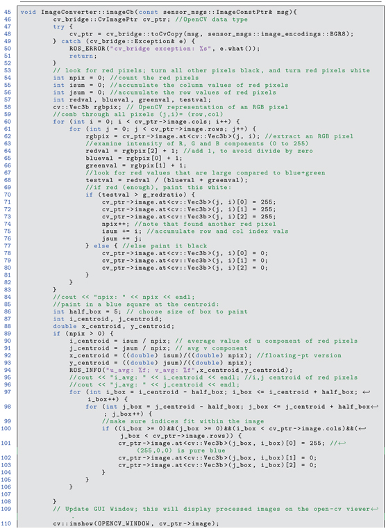

Listing 6.3 find_red_pixels.cpp: C++ code to find centroid of red pixels, method implementation

Listing 6.4 find_red_pixels.cpp: C++ code to find centroid of red pixels, main program
In findredpixels.cpp, lines 6 through 11 bring in the necessary headers for ROS, OpenCV, sensor messages, and ROS-OpenCV conversions. The main program (lines 119 through 133) merely instantiates an object of class ImageConverter, sets a global threshold parameter, then goes into a timed loop with spins. All of the computation in this node is done by callbacks defined within the ImageConverter class.
The ImageConverter class is defined in lines 18 through 43. This class has member variables (lines 20 through 22) that include a publisher and subscriber as defined in the imagetransport library, as well as an instantiation of an ImageTransport object. In the constructor (lines 26 through 34), the image publisher is set to publish to the topic imageconverter/outputvideo, and the subscriber is set to invoke the callback function imageCb upon receipt of messages on topic simplecamera/imageraw.
The actual work is performed in the body of the callback function, lines 44 through 117. Line 46:

OpenCV, cv_bridge defines a pointer to an image that is compatible with OpenCV. Data at this pointer is populated by translating the input ROS message msg into a compatible OpenCV image matrix in the format of an RGB image, with each color encoded as eight bits, using the code:

Lines 60 through 83 correspond to a nested loop through all rows and columns of the image, examining RGB contents of each pixel with a line of the form:

The redness of a pixel is chosen to be computed relative to the green and blue values, as evaluated by lines 64 through 66:

If the red component is at least 10 times stronger than the combined green and blue components, the pixel is judged to be sufficiently red. (This is an arbitrary metric and threshold; alternative metrics may be used.)
Lines 71 through 73 show how to set the RGB components of a pixel to saturation, corresponding to a maximally bright white pixel. Lines 78 through 80, conversely, set all RGB components to 0 to specify a black pixel. While combing through all pixels of the copied input image, lines 74 through 76 keep track of the total number of pixels judged to be sufficiently red, while summing the respective row and column indices. After evaluating all pixels in the image, the centroid of the red pixels is computed (lines 89 through 93).
Lines 97 through 106 alter the B/W image to display a square of blue pixels at the computed red-pixel centroid. This processed image is displayed in a native OpenCV image-display window using lines 110 and 111. The same image is published on a ROS topic using line 116:

The ROS-published image can be viewed by running:

The example code can be used with any image stream. For illustration, we can re-use our stereo camera model by running:

Next, add a small red block for the cameras to observe with:

This places a small, red block at (0, 0, 0.1) with respect to the left stereo camera’s frame. The findredpixels code example can now be run using the following launch file:

This launch file starts the imageview node, re-mapping its input topic to the left-camera topic /stereocamera/left/imageraw. This brings up a display window that shows the raw image from the left stereo camera. Additionally, this launch file starts up our example node findredpixels from package exampleopencv and re-maps the input topic from simplecamera/imageraw to /stereocamera/left/imageraw. The result shown in Fig 6.6 shows the Gazebo view with stereo cameras and a small red block centered below the left camera.
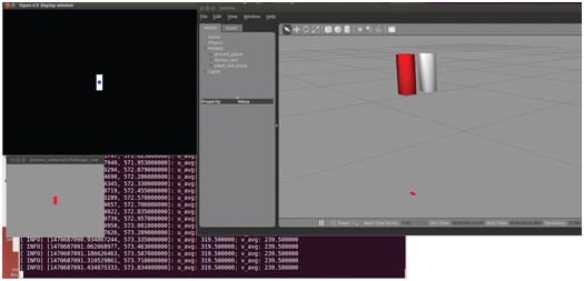
Figure 6.6 Result of running find_red_pixels on left-camera view of red block.
The imageview node shows a display of the raw video from the left camera, which shows a red rectangle centered in the field of view. The OpenCV display window shows the result of the image processing. There is a white rectangle centered in a black background, and the centroid of this white rectangle is marked with a blue square, as expected. The terminal prints the coordinates of this centroid (319.5, 239.5), which is in the middle of the field of view of the virtual image sensor.
The image displayed in the OpenCV display window is also published on the ROS topic /imageconverter/outputvideo. This can be verified by running another instance of imageview with input topic remapped to /imageconverter/outputvideo. Publishing intermediate steps of image processing can be useful for visualizing the behavior of an image pipeline to aid tuning and debugging.
In the example code, ros::spinOnce() is executed by the main program at 10 Hz. The input video rate, however, is 30 Hz. As a result, the example code only operates on every third frame. This can be a handy technique for reducing computational demand. A simpler and more effective means of reducing both bandwidth and CPU burden is throttling, which can be invoked using rqtreconfigure. Within this GUI, under the topic image throttling stereocamera/left, the GUI displays a slider for imager_rate. If the value is reduced to 1.0, imager_rate frames will be published only at 1.0 Hz. Using this GUI for throttling image rates can be convenient for interactively evaluating a good compromise for image rates.
6.4.2 Example OpenCV: finding edges
OpenCV, edge finding The previous example performed operations on individual pixels. More commonly with OpenCV, one uses existing higher-level functions. As an example, consider the source code findfeatures.cpp, which finds edges in images using a Canny filter. This example code follows the findredpixels code, with the addition of the following lines inserted into function imageCb() of findredpixels.

This code instantiates two OpenCV image matrices, grayimage and contours. The code line:

converts the received RGB image into a gray-scale image. This is necessary because edge detection on color images is not well defined. The gray-scale image is then used to compute an output image called contours using the function cv::Canny(). This function OpenCV, Canny edge filter takes two tuning parameters, a low threshold and a high threshold, which can be adjusted to find strong lines while rejecting noise. For the example image, which is black or white, the Canny filter will not be sensitive to these values, though these would be important in more realistic scenes, such as finding lines on a highway. The contour image is displayed in the OpenCV display window. (Original line 110, which displayed the processed image with blue-square centroid, has been commented out.) This example can be run much as before, with:

Next, add a small red block for the cameras to observe with:

Instead of launching findredpixelsleftcam.launch, use:

This starts the node findfeatures, performs the necessary topic re-mapping and starts imageview. With these steps, the output appears as in Fig 6.7. As desired, the OpenCV image displays the detected edges, which correspond to the edges of the block.

Figure 6.7 Result of running Canny edge detection on left-camera view of a red block.
While this is only a simple example of OpenCV capabilities, it illustrates how images can be processed with both low and high-level functions and how OpenCV can be integrated with ROS. Many advanced, open-source ROS packages exist using OpenCV, such as camera calibration, visual odometry, lane finding, facial recognition, and object recognition. Existing non-ROS OpenCV solutions can be ported to ROS with relative ease using cvbridge, and thus much prior effort can be leveraged with ROS.
6.5 Wrap-Up
This chapter introduced several fundamental concepts for using cameras in ROS. Conventions have been presented for assigning coordinate frames to cameras and reconciling these with sensor-plane pixel coordinates. A step toward getting physical coordinates from camera images is intrinsic camera calibration. ROS uses the conventions of OpenCV for representing intrinsic camera calibration. ROS packages support performing camera calibration, e.g. using checkerboard-style calibration templates. Results of intrinsic calibration are published on ROS camerainfo topics.
Camera calibration support in ROS is extended to stereo cameras. The results include individual camera intrinsic parameters, rectification parameters and identification of a baseline between transformed (rectified) images. The value of calibrating stereo cameras is that it becomes possible to infer 3-D coordinates of points of interest using multiple camera views.
Use of OpenCV for low-level image processing was introduced very briefly. OpenCV has an extensive library of image-processing functions, and these can be used within ROS nodes by following the integration steps presented in this chapter. Use of OpenCV functions with ROS will be introduced further in Chapter in the context of computing depth maps from stereo images.
1 Specification of frames for use with the “multicamera” plug-in is non-intuitive–presumably a bug in this plug-in. Some contortions with intermediate frames were required to achieve the desired camera poses and image-plane orientations.