CHAPTER 13
Arm Motion Planning
CONTENTS
13.1 Cartesian motion planning
13.2 Dynamic programming for joint-space planning
13.3 Cartesian-motion action servers
INTRODUCTION
Robot arm motion planning is a broad field with a variety of sub-problems. For example, one may be concerned with the optimal trajectory a robot can execute to get from some start pose to some final pose in minimum time, subject to constraints on the actuator efforts and joint ranges of motion. Another variant is planning arm motions that optimize the mechanical advantage of available actuators, e.g. as in weight lifting. A common problem is planning how to command a robot’s joints to move from an initial pose to a final pose (expressed either in joint space or in task space) while avoiding collisions (with the robot or with entities in the environment). The task to be performed may require a specified end-effector trajectory, e.g. as in laser cutting, sealant dispensing, or seam welding. In such cases, the velocity of the endpoint may be constrained by the task (e.g. for optimal material removal rates, torch speeds or dispensing rates). In demanding cases, motion planning must be performed in real time, e.g. to generate motion to catch a ball. At the other extreme, some motion plans for stereotyped behaviors (e.g. folding arms into a compact pose for transportation) may be computed offline with the results saved for execution as a rote skill. In cases of large communication latency, supervisory control may be the best approach. In this case, one may plan a motion and preview the result in simulation before committing the remote system to execute the approved plan.
Arm motion planning packages exist in ROS, and the sophistication and breadth of options may be expected to grow. In the current context, a single example planning approach will be described to illustrate how arm motion planning can integrate within a ROS-based hierarchy.
The example planning problem considered here assumes that one has a specified six-DOF path in Cartesian space that the robot’s tool flange must satisfy. For example, a seven-DOF arm may be required to move a knife blade along a specified path (along a workpiece) while maintaining a specified orientation of the knife (with respect to the workpiece), equivalently constraining six-DOF poses of the tool flange. It will be assumed that the Cartesian path can be adequately approximated by sequential samples along the continuous path. At each sample point along the path, the seven-DOF arm typically would have infinitely many inverse-kinematic options. Pragmatically, this may be approximated by sampled IK solutions, on the order of hundreds of options per Cartesian knot point. Even in this simplified scenario, the planning problem can be intimidating. For example, if there were 100 samples along the Cartesian trajectory and 200 IK solutions are computed for each such pose, there would be joint-space path options, which is overwhelmingly large.
Fortunately, this planning problem can be simplified dramatically using dynamic programming. The approach described here is composed of two layers: a Cartesian-space planner and an underlying joint-space planner.
13.1 Cartesian motion planning
The package cartesianplanner contains the source files for multiple Cartesian planners, including arm7dofcartesianplanner.cpp, ur10cartesianplanner.cpp, and baxtercartesianplanner.cpp, which define respective planning libraries for the seven-DOF arm, a Universal Robots UR10 arm, and the Baxter robot. The role of these libraries is to sample points along a Cartesian path, compute IK options for each sampled pose along the path, and (with the help of the joint-space planner) find the optimal sequence of joint-space solutions to traverse the desired Cartesian path.
In general, the Cartesian path to be followed is task dependent. The cartesianplanner is illustrative of how to sample a path and compute an attractive joint-space trajectory, but it is limited in its generality. The Cartesian planners described here have multiple motion-planning options:
- Specify a start pose, qvec, in joint-space coordinates, and specify a goal pose in Cartesian space. Compute a joint-space trajectory from the start angles to one of the IK solutions for the goal pose.
- Specify a start pose, qvec, in joint space, and specify a goal pose in Cartesian space. Compute a Cartesian trajectory by sampling points along a straight-line path. A trajectory will be generated such that desired final orientation of the gripper will be obtained quickly, then preserved throughout the linear move.
- Specify a start pose, qvec, and a desired delta-p Cartesian motion. Sampled Cartesian poses will be generated starting from the initial pose and translating in a straight line by the specified displacement vector while holding orientation fixed at the initial orientation.
- Specify Cartesian start and end poses with respect to the arm’s base. Only the orientation of the end pose will be considered. Orientation of start pose is ignored. A sequence of Cartesian poses is generated that maintains constant orientation while moving in a straight line from the start position to the end position.
The node examplearm7dofcartpathplannermain.cpp shows how to use the Cartesian planner arm7dofcartesianplanner.cpp, which relies on support from the corresponding kinematics library arm7doffkik and from the generic jointspaceplanner. Similarly, respective example main programs are provided for the Baxter robot and for the Universal Robots UR10 robot.
Running the node examplearm7dofcartpathplannermain will produce an output file arm7dofposes.path of joint-space poses that produce Cartesian motion with the tool flange orientation constant. In this example, the desired motion specifications are hard-coded in the main program, corresponding to maintaining orientation of the tool flange pointing up while translating from to at constant and . Samples along this path are computed every 5 cm. These path specification values can be edited to test alternative motions. With a roscore running, the seven-DOF arm planner example can be run with:

For this example, 60 samples are computed along the Cartesian path. At each sample point, inverse-kinematic options are computed at increments of 0.1 rad of the base joint. This results in roughly 200 IK solutions per Cartesian sample point (ranging from 130 to 285 IK solutions at each Cartesian pose, for this example).
Key lines of the code examplearm7dofcartpathplannermain.cpp are:
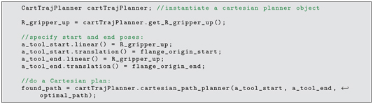
The planner option invoked in this example is specification of both start and end Cartesian poses. After calling cartesianpathplanner(), a joint-space plan will be returned in optimalpath. This plan is written to an output file called arm7dofposes.path, which consists of 61 lines (one for each Cartesian sample point), the first few lines of which are:
Each line specifies seven joint angles corresponding to a joint-space pose that is an IK solution of the corresponding desired Cartesian-space pose. Selection of optimal joint-space poses from among the candidate IK solutions is performed by a supporting library, the joint-space planner, which will be discussed next.
The planning libraries can be used as in this example for offline planning. Alternatively, the planning libraries can be used within action servers that perform motion planning and execution on demand. This option will be discussed further, after introducing a generic joint-space planning technique.
13.2 Dynamic programming for joint-space planning
Finding optimal joint-space solutions from among IK options can be challenging. A dynamic-programming approach to joint-space planning described here is applicable to a wide array of robots, at least for low-dimensional null spaces, such as seven-DOF arms.
For example, the motion plan for a seven-DOF arm illustrated by examplearm7dofcartpathplannermain.cpp results in 61 Cartesian samples, each of which has between 130 and 285 joint-space IK options. For each Cartesian sample point, a single IK solution must be chosen. However, these cannot be selected independently within each Cartesian sample point. Transitions between successive sample points must result in smooth motion, i.e. no large jumps in joint angles. Avoiding large jumps is not as simple as looking one step ahead, as invoking a greedy algorithm, since such an approach can lead to trajectories that result in poor options (large jumps) downstream. Instead, the entire path must be considered in context.

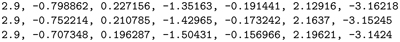
Figure 13.1 Conceptualization of a feed-forward network dynamic-programming problem
An approach to finding optimal sequences of joint-space solutions among a large number of options is dynamic programming. Conceptually, consider the feed-forward graph in Fig 13.1. The example network shown consists of six layers (columns), each comprised of some number of nodes (circles within each column). The network is feed-forward in the following sense. The m’th node in layer l, denoted as node , may have a link from to the n’th node in layer (node ). However, node has no link to any node in any layer other than layer . (e.g. links are never directed backward, nor do they skip over subsequent layers).
A path within this network starts at some node in layer L1 and concludes at some node in layer L6, visiting a total of six nodes (including start and finish) in the path. Any such path has an associated cost C that is the sum of state costs and transition costs. A state cost is a cost associated with passing through a given node ( for node m in layer l). A transition cost is the cost associated with following a link from node to node , which may be referred to as transition cost (e.g. as labelled in Fig 13.1). The path cost C is a scalar consisting of the sum of all state and transition costs (six state costs and five transition costs, in this example). Thus a candidate path can be scored with a penalty function of path cost. The optimization objective of the proposed problem is to find the path from L1 to L6 that has the minimum path cost.
With respect to our joint-space planning problem, we can interpret each layer as a six-DOF task-space pose sampled along a specified Cartesian path. The objective is to move the tool flange forward along this path, e.g. performing a cutting operation, and we can label (e.g.) six points along this path sequentially. For a task such as cutting (or drawing, welding, scribing, glue-dispensing, etc.) it would not make sense to skip over any of these points nor to ever go backward. Rather, each of the Cartesian subgoals must be achieved in sequence. We require that our end effector visit each of the Cartesian poses. However, computing inverse kinematics, we find that there are multiple joint-space solutions that achieve pose l. We may refer to the m’th joint-space solution at the l’th Cartesian pose to be node . (Depending on the chosen sampling resolution, we may consider hundreds of IK alternatives at each task-space sample or layer). Each node within our network describes a unique joint-space pose of the robot. A sequence of nodes, chosen 1 from each layer consecutively, describes a (discretized) joint-space trajectory that is guaranteed to pass through the sequential Cartesian-space samples along the task-space trajectory.
The state cost for a given node in this context may be scored by multiple criteria. For example, a robot pose that results in a self collision or a collision with the environment may be assigned a cost of infinity (or, more simply, removed from the network altogether). A node (pose) that is a near collision may have a high state cost. Nodes that are near singularities might also be penalized. Other pose-dependent criteria might also be considered. Transition costs should penalize large moves. For example, a path that included moving the base joint by moving from layer l to layer would result in high accelerations of high-inertia joints, which would be slow, disruptive, and presumably would result in wild tool-flange gyrations while moving only a short distance along the Cartesian path. Similarly, a sudden wrist flip from layer l to layer would be unacceptable, although the IK solutions may be correct at both of these layers. Thus, large changes in joint angles from layer to layer should be penalized.
Different optimal path solutions will result from different strategies of assigning state and transition penalties. The designer must choose how to assign costs to joint-space poses, how to assign transition costs, the number and locations of the Cartesian-space sample points (layers), and how many IK solutions (nodes) to consider at each sample point. Having cast the planning problem as a feed-forward graph, we can apply graph-solving techniques to our abstracted problem, yielding a sequence of joint-space poses that advance the robot through the chosen Cartesian-space poses.
For this type of graph, dynamic programming can be applied effectively. The process is as follows. Working backward from the final layer, each node will be assigned a cost to go. For the final layer, the cost to go is simply the state cost associated with each final-layer node.
Backing up to layer (layer L5, in our example), each node in this layer is assigned a cost to go. For our example, for node 1 in layer L5, , there are only two options: to transition to node at a cost of , or transition to node at a cost of . The cost to go for node will be assigned the minimum of these two options, which we may label as . The cost to go for node is computed similarly, resulting in an assigned value .
Continuing to work backward through the network, when computing cost to go for nodes in layer l, we may assume that the cost to go has already been computed for all nodes in layer . To compute the cost to go for node m in layer l, , consider each node n in layer l+1 and compute the corresponding cost . Find the minimum cost (over all options in layer ) among these options and assign it to . In this process, a cost to go is computed for every node in the network, and computing these costs is comparably efficient at every layer.
Given cost to go assignments for every node, the optimal path through the network can be found by following the steepest gradient of costs through the network.
A simple numerical example is illustrated with the help of Figs 13.2 through 13.6.
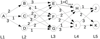
Figure 13.2 Simple numerical example of dynamic programming consisting of five layers with transition costs assigned to each allowed transition

Figure 13.3 First step of solution process. Minimum cost to go is computed for nodes H and I. Two of the four links from layer four to layer five are removed because they are provably suboptimal

Figure 13.4 Second step of solution process. Minimum cost to go is computed for nodes E, F and G in layer 3 (costs 2, 3 and 2, respectively). Three of the six links have been pruned, leaving only the single optimal option for each node in layer three. It can be seen at this point that node I will not be involved in the optimal solution.

Figure 13.5 Third step of solution process. Minimum cost to go is computed for nodes B, C and D in layer two (costs 4, 4 and 3, respectively). Six of the nine links have been pruned, leaving only the single optimal option for each node in layer two.
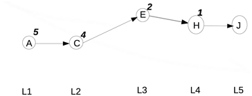
Figure 13.6 Final step of solution process. Minimum cost to go is computed from node A. Only a single path through the network constituting the optimal solution survives.
This sequence of views shows how the cost to go computation propagates backward from the goal states. As the cost to go is computed, many of the options can be eliminated as provably suboptimal in the context of a globally optimal solution. Typically, a single link will survive the cost to go optimization at each layer of computation. In this simple example with integer transition costs, ties could exist, resulting in multiple surviving links from each such incremental optimization. In practice, however, the cost will be a floating-point value and ties will not occur.
In the illustrated example, it becomes clear early on that node I cannot be part of the optimal solution, and thus the goal node must be node J. Working backward through the layers, links are pruned and incremental transition costs are replaced with the optimal cost to go associated with each node. As the process sweeps back to the starting layer, a single path through the network results (Fig 13.6). This solution process is quite efficient, and the resulting path is provably optimal.
A library that performs this optimal-path computation is in the package jointspaceplanner.
This planner assumes all state costs are merely zero (with the presumption that dangerous poses have already been removed from the network). Transition costs are assigned to be a weighted sum of squares of delta joint angles corresponding to a transition. One must provide an entire network and a vector of weights (associated with joints) to the planner constructor, and the planner will return the optimal path through the network. The network passed to the solver is represented as:

The pathoptions argument is a (std) vector of (std) vectors of (Eigen) vectors. The outermost vector contains L elements corresponding to L layers in the network. Each layer within this vector contains a vector of nodes (IK options at this point along the trajectory). The number of nodes within a layer may vary from layer to layer. Each node within a layer is an N-jointed IK solution, expressed as an Eigen-type vector. The network solver is written to accommodate arbitrary dimensions in terms of number of layers, number of nodes in any layer, and number of dimensions of each node. However, care should be taken to avoid excessive numbers of layers and numbers of nodes per layer, as the planning can become slow.
In the example examplearm7dofcartpathplannermain.cpp, a seven-DOF robot is considered moving along a Cartesian path sampled every 5 cm, resulting in 61 layers (including start and end poses). Each layer has between 130 and 285 IK joint-space options. On one core of a 2 GHz i7 Intel processor, the planning process requires about 8 sec, which includes approximately 3 sec to compute approximately 13,000 IK solutions and about 5 sec to find the minimum-cost path through the resulting network.
The result of the example plan is the file arm7dofposes.path, which lists the seven-DOF joint angles recommended for each of the 61 steps along the Cartesian path.
The example Cartesian planners in package cartesianplanner, including 7DOFarm, UR10 and Baxter, all use the same joint-space planner library described here. The library is flexible enough to accommodate any number of joints, any number of IK solutions per Cartesian sample point, and any number of Cartesian sample points along a Cartesian path. However, excessively large networks will require correspondingly large computation times.
It should be noted, however, that the simple joint-space planning optimization illustrated here does not take into consideration potential collisions, either with the environment or with the robot’s own body. Joint-space solutions that would result in collisions should be removed from the graph before planning a path through the network.
13.3 Cartesian-motion action servers
In Section 13.1, Cartesian motion planning libraries were introduced. Each such motion library is customized for a specific robot type. However, the objective is the same in each case: a gripper or tool is to be moved in space to a destination pose, often constrained to move along a Cartesian path. Ideally, this can be accomplished with commands from a higher level that are robot agnostic. An example approach to this uses Cartesian motion action servers.
In the cartesianplanner package, the nodes baxterrtarmcartmoveas.cpp and ur10cartmoveas.cpp use their respective Cartesian planner libraries and they present an action-server interface called cartMoveActionServer. Action clients can communicate with these action servers using a generic action message, defined in cartmove.action in the cartesianplanner package. This action message includes the following mnemonics in the goal field:
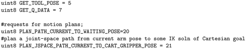
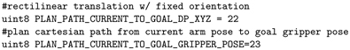
Each of these is an action code that can be specified by a client.
Components of the goal message are:
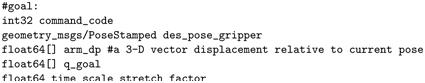
A client should fill in the commandcode field with one of the defined action-code values. For the case of PLANPATHCURRENTTOWAITINGPOSE, no additional fields need to be filled in. For requesting either a joint-space or Cartesian-space plan to a goal pose, the client must specify the corresponding command code in the goal message and must also specify the desired gripper pose in the desposegripper field. If requesting a relative motion along a specified vector, the desposegripper field is not needed, but the armdp field must be filled in. (Joint-space goal specifications are also possible, although this mode is less general and should be avoided).
An example client program that uses this action interface is examplegenericcartmoveac.cpp in the cartesianplanner package. This node instantiates an action client that connects to the action server cartMoveActionServer (through use of the library cartmotioncommander) and communicates via the action message cartmove.action. This client illustrates invoking various actions offered by the Cartesian-motion action server, including: planning and executing a path to a pre-defined waiting pose; planning and executing a path to an absolute tool pose; and planning and executing a Cartesian motion relative to the current tool pose. The class ArmMotionCommander in the cartmotioncommander library encapsulates details for invoking these behaviors, including populating a cartmove goal message, sending this message to the action server, and returning the response code received by the callback function. This simplifies the action client code, as in the snippet below from examplegenericcartmoveac.cpp.

These lines of code invoke the behaviors of moving to a pre-defined waiting pose, then moving to a specified tool pose along a Cartesian path. At this level of abstraction, the client does not need to be aware of what type of robot it is controlling. Rather, the client can focus on moving a tool in task space while leaving details of inverse kinematics and Cartesian-space planning to the action server. In fact, the example generic action client works equally well with the Baxter robot or with the UR10 robot with no changes, in spite of the fact that these robots have very different kinematic properties, including numbers of joints.
One minor complication is that the relevant frame names (e.g. gripper frame and base-link frame) of different robots may have different names, which limits the re-usability of application code. A fix for this is to define additional frames on these robots that present generic names. For example, the Baxter robot’s right arm has a gripper with a frame between the fingertips called rightgripper. The UR10 robot does not have such a frame name. The last link of the UR10 has a frame called tool0. Further, Baxter robot kinematics is computed with respect to the torso frame, whereas the UR10 robot has no torso frame. Instead, UR10 kinematics is computed with respect to its baselink frame. To have the Baxter robot present a common interface, baxterstatictransforms.launch from the cartesianplanner package is run. This launch file consists merely of:
By running this launch file, two additional frames are published on tf: genericgripperframe and systemrefframe. The generic gripper frame in this case is prescribed to be identical to the rightgripper frame, since the argument list specifies x, y, z = 0, 0, 0, and quaternion x, y, z, w = 0, 0, 0, 1. With this publication, one can refer to genericgripperframe as a synonym for rightgripper to invoke planning and motion execution. The other frame published, systemrefframe, relates a generic reference frame name to the relevant Baxter frame, torso. In this case, the torso is specified to be 0.91 m above the system reference frame (which is defined to be on the ground plane). Object poses can be defined with respect to the system reference frame, and the transform from system reference frame to torso frame can be calibrated to correspond to the mounting height of the robot.
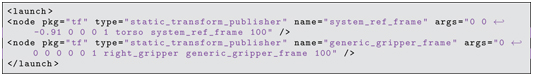
Correspondingly for the UR10, the model frames to be referenced are baselink and tool0 (unless a gripper is added to the model, in which case tool0 should be substituted for an appropriate frame on the gripper). These frames are associated with systemrefframe and genericgripperframe, respectively. This is done by launching ur10statictransforms.launch within the cartesianplanner package. The contents of this launch file are:

Launching this file results in genericgripperframe being synonymous with tool0, and systemrefframe being synonymous with the world frame. This assumes that the robot is launched with a transform describing the robot’s baselink with respect to the world frame. With these additional transforms, one can control the UR10 by referring to the genericgripperframe in the systemrefframe.
The example generic Cartesian-move action client can be run on the UR10 robot as follows. First, start a UR10 simulation with:

Then, start the static transform publications for gripper and reference frames with:

Start a Cartesian-move action server for the UR10 robot by running:

At this point, the robot is ready to receive and act on Cartesian-motion planning and execution goals. The simple example action client can be run with:

This example code will prompt the user for input, including asking for a desired delta-z value for a Cartesian motion. The action client will run to conclusion, but the action server will persist, ready to accept new goals from new action clients.
To run the same, generic Cartesian-move client node with the Baxter robot, first start the Baxter robot simulation with:

Wait for the start-up to conclude (which may take 30 seconds, or so). Then enable the motors with the command:

Start a trajectory-streamer action server with:

Start the transforms that define the generic gripper frame and the system reference frame:

Start the Cartesian-motion action server for Baxter’s right arm:

The Baxter robot is now ready to accept Cartesian-motion goals from an action client. The generic action client can be run, identical to the case of the UR10 robot, with:

Running this node results in Baxter’s right-gripper frame executing Cartesian trajectories in exactly the same way as the UR10 moves its tool0 frame. This ability to refer to Cartesian-space motions of generic gripper frames offers the possibility of writing higher-level code that is independent of any specific robot arm design. By abstracting the programming problem in this way, the programmer can focus on thinking in task space while ignoring the details of how any one robot could carry out the desired task-space trajectories. This will be discussed further in the context of an objectgrabber package, after introducing some further detail of the Baxter simulator.
13.4 Wrap-Up
Controlling a robot arm ultimately reduces to specifying a stream of coordinated joint-angle commands in time. Computing a desirable motion can be highly complex, and arm motion planning is a broad and open field. One example planning approach that is applicable to kinematically redundant robots (with low null-space dimensionality) was presented using dynamic programming. The result of the planning computation is a trajectory message, which can be communicated to a trajectory action server running on the robot. It was shown how Cartesian-motion planners can be embedded in action servers, and these action servers can refer to generic gripper and system reference frames. Such an approach supports the possibility of writing generic action client nodes that focus on task-space operations and are re-usable across multiple robot designs.
We next consider development of these concepts specifically with respect to the Baxter robot.