CHAPTER 12
Robot Arm Kinematics
CONTENTS
INTRODUCTION
Robot arm kinematics is a starting point for most textbooks in robotics. A fundamental question is, given a set of joint displacements, where is the end effector in space? To be explicit, one must define reference frames. A frame of interest on a robot may be its tool flange, or some point on a tool tip (e.g. welder, laser, glue dispenser, grinder, ...) or a frame defined with respect to a gripper. It is useful to compute the pose of the defined frame of interest with respect to the robot’s base frame. In a separate transform, one can express the robot’s base frame with respect to a defined world frame. The task of computing the pose of a robot’s end effector with respect to its base frame given a set of joint displacements constitutes forward kinematics. For open kinematic chains (i.e. most robot arms), forward kinematics is always simple to compute, yielding a unique, unambiguous pose as a function of joint displacements.
While forward kinematics is relatively simple, the more relevant question is typically the inverse: given a desired pose of the end effector frame, what set of joint angles will achieve this objective? Solving this inverse kinematics relationship is plagued with problems. There may be no viable solutions (goal is not reachable), there may be a finite number of equally valid solutions at very different sets of joint angles (typical for six-DOF robots), or there may be an infinity of solutions (typical for robots with more than six joints). Further, while forward kinematics solutions can be obtained using a standard procedure, solving for inverse kinematic solutions may require ad hoc algorithms exploiting creative insights.
The kinematics-and-dynamics package KDL (see, e.g. http://www.w3.org/1999/xlink) is a popular tool for computing forward kinematics and robot dynamics. One of its capabilities is that it can reference a robot model on the parameter server to obtain the information necessary to compute forward kinematics. Thus, any open-chain robot in ROS already has a corresponding forward kinematics solver (via KDL). KDL also computes Jacobians (between any two named frames).
Unfortunately, the more useful and more difficult problem of inverse kinematics is not handled well in general. If the robot of interest has specific properties (e.g. six DOFs with a spherical wrist), inverse kinematic solutions can be computed analytically, yielding exact expressions for all possible solutions. However, robots with redundant kinematics (more than six DOFs) are increasingly popular, due to their enhanced dexterous workspace, and this makes computing inverse kinematics ambiguous. Further, many robot designs do not conform to the equivalent of a spherical wrist, and for such designs, there may be no known analytic inverse kinematics solution.
Numerical techniques (gradient search using a kinematic Jacobian) are often employed when analytic inverse kinematic solutions are not available. As is typical with numerical searches, this approach can be slow, fail to converge, get stuck in local minima, and (when successful) typically returns a single solution when multiple solutions or an infinity of solutions exist.
When working with a particular robot, if an inverse kinematics package is available, the available solution may be sufficient. If a suitable package is not already available, it may be necessary to design one.
This chapter will introduce examples of forward and inverse kinematics libraries and use these to illustrate common issues in robot kinematics.
12.1 Forward kinematics
A simple example to illustrate kinematics is in the package rrbot. This robot model borrows from the on-line tutorial at http://www.w3.org/1999/xlink for the rrbot (a two-DOF robot with two revolute joints). In the subdirectory model the file rrbot.xacro defines a simple, planar manipulator with three links and two joints. Figure 12.1 shows Gazebo and rviz views of this robot, which was launched using:


Figure 12.1 Gazebo and rviz views of rrbot
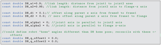
The rrbot has frames defined for each of its links. To be consistent with Denavit-Hartenberg convention, the frames were defined such that the z axes pass through revolute joint axes (for joints 1 and 2), as follows:
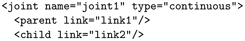
By defining this frame, tf will compute transformations out to this frame of interest.
The fictitious link flange is defined simply as:

Since the link flange is connected by a static joint, it is not necessary to define inertial, visual or collision components. The same technique is useful for modeling mounting sensors (rigidly) to robots or defining tool frames on specific end effectors.
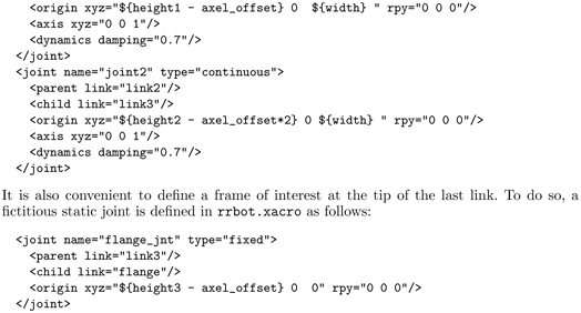
With the above joint definitions, the equivalent Denavit-Hartenberg parameters, as defined in the header file rrbot/include/rrbot/rrbotkinematics.h, are:
Converting between a URDF and DH models can be confusing. In the present case, having defined the joint axes consistent with DH convention, the z axes of DH frames 1 and 2 are parallel (as well as the z axis of the flange frame), and consequently the alpha angles are zero, and the a parameters are the link lengths. Since there is an offset from link1 to link2 along the z direction, there is also a non-zero d1 parameter.
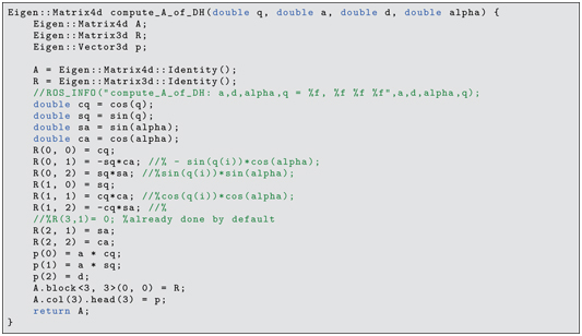
In the rrbot package, the source file rrbotfkik.cpp compiles to a library that computes forward and inverse kinematics for the rrbot. The function computeAofDH() returns a 4 4 coordinate-transform matrix, as described in Chapter 4. In general, a coordinate transform between successive DH frames follows from specification of the four DH parameters, as shown in computeAofDH().
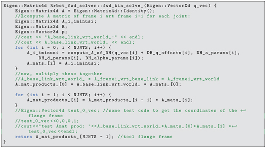
A general procedure for computing forward kinematics simply involves computing each successive 4 4 transformation matrix, then multiplying these matrices together. This is implemented in the function fwdkinsolve() within the rrbotfkik.cpp library as follows:
This same forward-kinematics code is applied as well to additional example robots in learningros/Part5, including a six-DOF ABB robot (model IRB120), the six-DOF Universal Robots UR10, the Baxter robot (with seven-DOF arms) and a robot model based on the NASA Goddard satellite-servicer arm (called arm7dof). To customize the forward kinematics code for a specific robot, it is necessary only to define the number of joints and values for the DH parameters in the respective header file. If using the KDL package, that step is not even necessary, since KDL will parse the robot model to obtain the parameter values.
Forward and inverse kinematics can be tested using the testrrbotfk.cpp test function. The rrbot, test function, and supporting tools are brought up with:

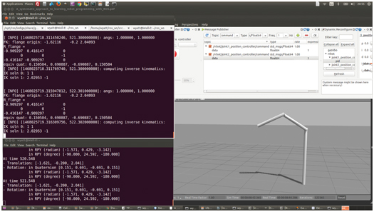
Figure 12.2 Gazebo, tf_echo and fk test nodes with rrbot
A screenshot with these nodes running is shown in Fig 12.2. The robot can be moved to arbitrary poses using rqtgui. In the example shown, the joints are both commanded to angles of 1.0 rad. The testrrbotfk node subscribes to jointstates and prints the published joint values, confirming that the robot is at the commanded joint angles. (In this test, gravity was set to zero, so there is no joint error from gravity droop.) Forward kinematics of the flange frame with respect to the base (world) frame is computed and displayed as:

To test this result, the tfecho node is run to get the flange frame with respect to the world frame. This function displays:
To the precision displayed, the results are identical.
A second, more realistic test can be run with:
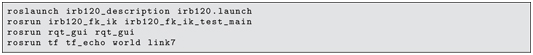

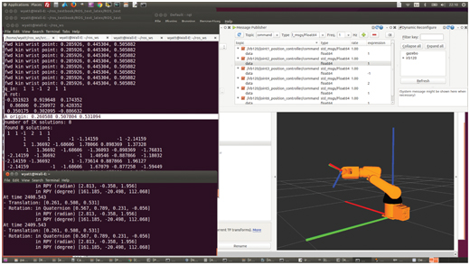
Figure 12.3 rviz, tf_echo and fk test of ABB IRB120
This launches a model of the ABB IRB120 industrial robot. Using rqtgui, the six joints are commanded to the values . The resulting pose is shown in Fig 12.3. The tfecho node prints out the pose of the flange frame (link7) with respect to the world. It displays:

The test node irb120fkiktestmain subscribes to the joint states and uses these values to compute forward kinematics. This node prints out:

Again, to the precision displayed, the results are identical. Additional spot checks yield similar results.
12.2 Inverse kinematics
The code used to compute forward kinematics for the two-DOF rrbot and the example six-DOF arm is virtually identical, except for the number of joints and the specific numerical values of the DH parameters. The algorithmic approach is valid in general for all open kinematic chains. In contrast, inverse kinematics can require robot-specific algorithms and may be problematic for handling multiple solutions, which is exacerbated with kinematically-redundant robots.
Starting with the two-DOF rrbot, inverse kinematics can be computed using the law of cosines. The rrbotfkik.cpp program includes a class for forward kinematics and a class for inverse kinematics. The inverse kinematics function iksolve() takes an argument for the desired end-effector pose (as an Eigen::Affine3 object), and it populates a std::vector of Eigen::Vector2 objects comprising alternative solutions. There can be 0, 1 or 2 solutions for the rrbot.
With only two degrees of freedom, it is (typically) only possible to satisfy two objectives. For example, one cannot find solutions for an arbitrary desired position (x, y, z) of the tool flange. The rrbot can only reach flange coordinates for which . If the requested flange position is (x, 0.2, z), then solutions may be possible.
The function iksolve() first calls solveforelbowang(), which returns 0, 1 or 2 reachable elbow (joint2) angles. These angles follow from the realization that the distance from the shoulder to the flange is a function only of joint2 (not joint1). The value of joint2 angle can be found from the law of cosines: . In this case, a and b are the lengths of the two movable links and c is the desired distance from the robot’s shoulder (joint1) to the tool flange (tip of distal link). These three lengths form a triangle, and the angle C is the angle opposite the leg with length c. This relationship can be solved for angle C using an inverse cosine. However, there are zero, one or two solutions for C in this equation. If, for example, a flange pose is requested that is beyond the reach of the robot (i.e. ), there are no solutions for C.
When the requested position is within reach of the robot, there are typically two solutions. (A special case occurs when the arm is fully extended, precisely reaching a desired position; in this case there is only one solution.) Most commonly, if there are any solutions, there are two solutions (commonly referred to as elbow up and elbow down).
For each of the elbow solutions, one can find the corresponding shoulder angle (joint1 angle) that achieves the desired flange position. This is computed using the function solveforshoulderang(), reduces the shoulder-angle problem to solving an equation of the form for the value of q. This equation occurs frequently in inverse-kinematics algorithms and is solved within the function solveKeqAcosplusBsin(K, A, B, qsolns). There is some ambiguity, though, since two solutions are obtained, and only one is consistent with a correct robot pose. For a given elbow angle, both candidate shoulder angles are tested using forward kinematics, and the correct shoulder angle is thus identified. Typically, if the desired point is reachable, there will be two valid solutions, and .
As an example, the desired flange position of:

has two solutions, as computed and displayed by testrrbotfk:
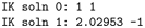
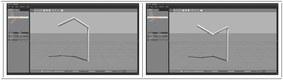
Figure 12.4 Two IK solutions for rrbot: elbow up and elbow down
These solutions are illustrated in Fig 12.4 Inverse kinematics for the ABB IRB120 is more complex. Fortunately, this robot design incorporates a spherical wrist. (A spherical wrist is a design for which the last three joint axes intersect in a point.) Existence of a spherical wrist simplifies the IK problem, since one can solve for position of the wrist point (the point of intersection of the last three joint axes) in terms of the proximal joints (joints 1, 2 and 3, in the case of the IRB120). Transformation matrices, law of cosines, and solutions of are again exploited to solve for joint-angles q1, q2 and q3. In addition to elbow-up and elbow-down solutions, the robot can also rotate 180 degrees about its turret (base) to reach backward to achieve two more elbow-up, elbow-down solutions. There thus can be four distinct solutions that place the wrist point at its desired position. For each of these solutions, the spherical wrist offers two distinct solutions. All together, these comprise eight IK solutions. A specific example for the IRB120 robot was run using the irb120fkiktestmain node, starting the robot at joint angles . Forward kinematics was computed, then this flange pose was used to generate inverse-kinematic solutions. For this case, there were eight solutions, including re-discovery of the original joint angles, . The eight solutions for this case are:
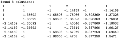
These solutions show that the first three joint angles appear twice in separate solutions, which differ only in the last three (wrist) joint angles. All eight of the solutions for this example are shown in Fig 12.5. The two distinct wrist solution for each combination of (q1, q2, q3) may not be easily discernible, but these solutions are quite distinct in (q4, q5, q6).

Figure 12.5 Example of eight IK solutions for ABB IRB120
Although the example shown has eight IK solutions, the number of solutions can vary. If a requested point is beyond the reach of the robot (or within the body of the robot) there will be no viable solutions. If IK solutions require moving one or more joints beyond their allowable range of motion, there will be fewer than eight valid solutions. If the desired pose is reachable at a singular pose (when two or more joints align such that their joint axes are colinear), there will be an infinity of IK solutions (describable as a function of the sum or difference of the joint angles of the aligned joints).
A related example is in package urfkik, which is a library of forward and inverse kinematics functions for the Universal Robots UR10 robot. This six-DOF robot does not have a spherical wrist, but an analytic inverse-kinematic method does exist. Typically, there are eight IK solutions for each desired tool flange pose (if reachable) within 0 to 360 degree joint angle ranges.
With an array of IK solutions, one requires an algorithmic means to choose among the solutions to execute one of them. Choosing a best solution can be ambiguous, but one expectation is that the robot will not jump suddenly, e.g. between elbow-up and elbow-down solutions, during execution of a trajectory.
How to choose among candidate solutions is even more challenging when the robot has more than six degrees of freedom (or, more generally, when the robot degrees of freedom is larger than the number of task constraints). In such cases, there is a continuum (or multiple, distinct continua) of solutions to choose from. An example is in arm7dof.
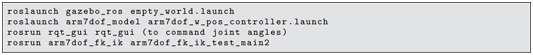
The robot model in arm7dofmodel is based on the NASA RESTORE arm design being considered for servicing satellites in space. A Gazebo view of a proposed NASA design is shown in Fig 12.6. Frame assignments for this seven-DOF arm are shown in Fig 12.7. The model in package arm7dofmodel is a simplified, abstracted version of the satellite servicer arm. This model (with a large disk appended to the tool flange) appears as in Fig 12.8. This design incorporates a spherical wrist, which simplifies the inverse-kinematics algorithm. For each solution of (q1, q2, q3, q4) that places the wrist point in a desired position, there are two solutions (q5, q6, q7) that achieve the desired flange pose (satisfying both desired position and orientation of the flange). However, if the desired wrist point is reachable, there is typically a continuum (or multiple, disconnected continua) of solutions in the space (q1, q2, q3, q4). 1
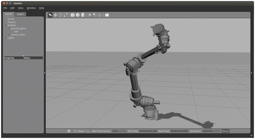
Figure 12.6 Proposed NASA satellite-servicer arm, Gazebo view

Figure 12.7 Proposed NASA satellite-servicer arm, rviz view with frames displayed
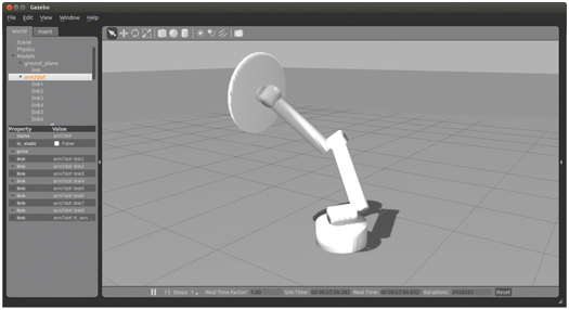
Figure 12.8 Approximation of proposed NASA satellite-servicer arm
An approach to inverse kinematics for this arm is presented in [2], in which solutions are obtained as a function of a free variable, such as the elbow-orbit angle or the base turret angle. The latter approach is taken here. Within the package arm7doffkik, a forward and inverse kinematics library contains a key function ikwristsolnsofq0(). This function accepts coordinates of a desired wrist point along with a desired turret angle (q1) and it returns all of the viable solutions for joint angles (q2, q3, q4). As with the ABB six-DOF robot, once q1 is constrained, only (these) three joints imply the wrist-point coordinates, and there can be up to four distinct solutions. Also like the ABB six-DOF robot, each of these wrist-point solutions theoretically has two solutions for (q5, q6, q7) (though these may or may not be reachable within the robot’s joint range-of-motion constraints). In at least some instances, there thus will be eight distinct, viable IK solutions (at given angle q1). For the pose in Fig 12.8, there are six distinct, reachable IK solutions at .
The choice of base angle, q1, for an optimal IK solution is unclear. In fact, the best choice of q1 may only be knowable in a broader context. To defer choosing a value of q1, one can compute IK solutions for a range of q1 candidates, sampled at some chosen resolution. The function iksolnssampledqs0() accepts a specified flange pose and fills in a (reference variable) std::vector of seven-DOF IK solutions. The sampling resolution of q1 is set by the assigned value of DQYAW, which is set to 0.1 rad in the header file arm7dofkinematics.h. For the pose shown in Fig 12.8, 228 valid IK solutions were computed at a sampling resolution of 0.1 rad over q1 from 0 to . This example was computed using the following code in package arm7doffkik:
Since all of these solutions are computed analytically, they present no numerical issues, such as failure to converge. Further, the analytic approach yields a large number of options, not simply a single solution (in contrast to a numerical approach). The solution process is also relatively efficient. For the example shown, computing 228 IK solutions required approximately 30 msec on a laptop using one core of a 2 GHz Intel i7.
The number of solutions expands dramatically in singular poses. Figure 12.7 shows the seven-DOF arm in a singular pose, for which the joint axis of joint 7 is colinear with the joint axis of joint 5. In such poses, given any solution, one can generate a space of solutions by rotating joint 7 by and simultaneously rotating joint 5 by , thus generating a continuum of solutions even at fixed q1.
For some robot arms, an analytic solution may not be known. In such cases, one must resort to numerical methods. If an approximate analytic solution is known, it can be useful to solve for approximate solutions and use these as starting points for a numerical search. In the numerical search, the manipulator Jacobian is a key component. Jacobians, like forward kinematics, are easy to compute and are well behaved. The example kinematic libraries provided include Jacobian computations.
12.3 Wrap-Up
This chapter has presented a brief overview of robot-arm forward and inverse kinematics. Forward kinematics for open kinematic chains has been solved in general. The tf package computes forward kinematics in real time, based on robot model information available in a URDF. The popular kinematics-and-dynamics package KDL also offers forward-kinematics solutions. Inverse kinematics, on the other hand, does not have a general solution, and for kinematically-redundant robots, there is an entire range of IK solution options. If a robot of interest does not already have an inverse-kinematic solution implemented in ROS, the developer may need to create one, as illustrated in the examples of this chapter.
Forward and inverse kinematics is only one step in motion control of robot arms. At a higher level of abstraction, one needs to plan a smooth sequence of robot arm poses that achieves some desirable behavior. The issue of robot arm motion planning is considered next.
1 By DH convention, joint-angle numbering starts at 1 at the most proximal joint and increments sequentially to the last joint. However, indexing in C++ starts from 0, and thus joint numbers are sometimes numbered from 0.