CHAPTER 4
Coordinate Transforms in ROS
CONTENTS
4.1 Introduction to coordinate transforms in ROS
4.4 Transforming ROS datatypes
INTRODUCTION
Reconciliation of coordinates is necessary to take advantage of sensor-driven behaviors, whether in simulation or in physical control. Coordinating data from multiple models and sensors is accomplished through coordinate transformations. Fortunately, ROS provides extensive support for coordinate transformations. Since transforms are ubiquitous in ROS and in robotics in general, it is important to have an understanding of how coordinate transforms are handled in ROS. coordinate transforms
4.1 Introduction to coordinate transforms in ROS
Coordinate frame transformations are fundamental to robotics. For articulated robot arms, full six-DOF transforms are required to compute gripper poses as a function of joint angles. Multiplication of sequential transforms, link by link, performs such computations. Sensor data, e.g. from cameras or LIDARs, is acquired in terms of the sensor’s own frame, and this data must be interpreted in terms of alternative frames (e.g. world frame or robot frame).
Any introductory robotics text will cover coordinate-frame assignments and transformations (e.g. [3,36]). A brief introduction to coordinate-frame transformations is given here, leading to ROS’s treatment of coordinate transforms.
A frame is defined by a point in 3-D space, , that is the frame’s origin, and three vectors: , and (which define the local , and axes, respectively). The axis vectors are normalized (have unit length), and they form a right-hand triad, such that crossed into equals : . coordinate frame
These three directional axes can be stacked side-by-side as column vectors, comprising a matrix, .
1
We can include the origin vector as well to define a matrix as:
2
orientation matrix
A useful trick to simplify mathematical operations is to define a homogeneous transformation matrix by converting the above matrix into a square matrix by adding a fourth row consisting of [ 0 0 0 1]. We will refer to this augmented matrix as a matrix:
3
homogeneous transformation matrix
Conveniently, matrices constructed as above (consistent with valid frame specifications) are always invertible. Further, computation of the inverse of a matrix is efficient.
Abstractly, one can refer to an origin and a set of orientation axes (vectors) without having to specify numerical values. However, to perform computations, numerical values are required. When numerical values are given, one must define the coordinate system in which the values are measured. For example, to specify the origin of frame B (i.e. point ) with respect to frame A, we can measure from the origin of frame A to the origin of frame B along three directions: the axis of frame A, the axis of frame A, and the axis of frame A. These measurements can be referred to explicitly as , , and , respectively. If we provided coordinates for the origin of frame B from any other viewpoint, the numerical values of the components of would be different.
Similarly, we can describe the components of frame B’s axis (correspondingly, and axes) with respect to frame A by measuring the x, y and z components along the respective axes of frame A.
Equivalently, this representation can be interpreted as the following operation. First, translate frame B such that its origin coincides with frame A, but do not change the orientation of frame B. The three axis vectors of frame B have tips that are unit length from the (common) origin. These define three distinct points in space, and each of these axis tips of frame B can be expressed as 3-D points, e.g. as measured in frame A. Equivalently, the tip of the axis of frame B is simply in the B frame and with respect to the A frame.
We can then state the position and orientation of frame B with respect to frame A as:
4
We can refer to the above matrix as “frame B with respect to frame A.”
Having labeled frames A and B, providing values for the elements of fully specifies the position and orientation of frame B with respect to frame A.
In addition to providing a means to explicitly declare the position and orientation of a frame (with respect to some named frame, e.g. frame B with respect to frame A), matrices can also be interpreted as operators. For example, if we know the position and orientation of frame C with respect to frame B, i.e. , and if we also know the position and orientation of frame B with respect to frame A, , we can compute the position and orientation of frame C with respect to frame A as follows:
5
That is, a simple matrix multiplication yields the desired transform. This process can be extended, e.g.:
6
In the above, the on the left-hand side can be interpreted column by column. For example, the fourth column (rows 1 through 3), contains the coordinates of the origin of frame F as measured with respect to frame A.
The notation of prefix superscripts and post subscripts provides a visual mnemonic to aid logical compatibility. The super and sub-scripts act like Lego™blocks, such that a subscript of a leading matrix must match the pre-superscript of the trailing matrix. Following this convention helps to keep transform operations consistent.
Since coordinate transforms are so common in robotics, ROS provides a powerful tf package for handling transforms. (See http://www.w3.org/1999/xlink.) Use of this package can be confusing, because tf performs considerable work. tf package tf topic
To examine the tf topic, we can start Gazebo with an empty world:

and then bring up our mobile robot with one-DOF arm:

This results in 18 topics published, including the topic tf. Issuing:

shows that the topic tf carries messages of type tf2_msgs/TFMessage.
Running:

tf2_msgs reveals that the tf2_msgs/TFMessage is organized as follows:
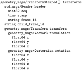
That is, this message contains a vector (variable-length array) of messages of type geometry_msgs/TransformStamped. TransformStamped
The ROS transform datatype is not identical to a homogeneous transformation matrix, but it carries equivalent information (and more). The ROS transform datatype contains a 3-D vector (equivalent to the fourth column of a transform) and a quaternion (an alternative representation of orientation). In addition, transform messages have time stamps, and they explicitly name the child frame and the parent frame (as text strings). child frame parent frame quaternion
There can be (and typically are) many publishers to the tf topic. Each publisher expresses a transform relationship, describing a named child frame with respect to a named parent frame. In the present example, Gazebo publishes to tf because, within the differential-drive plug-in, this was requested with the publishWheelTF option:

(Note that publishWheelJointState was also enabled for this plug-in). publishWheelTF publishWheelJointState
Running:

shows that the tf topic is updated at 300 Hz. Examining the output of tf with:

shows that the transforms component (a variable-length array) of this message includes multiple, individual transform relationships. An (abbreviated) excerpt from the tf echo output is:
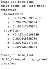
The left_wheel link has a defined reference frame, as does the base_link. From the tf output, we see that a transform is expressed between the base_link frame and the left_wheel frame (and similarly between the base_link frame and the right_wheel frame). The transform from the base_link frame to the left_wheel frame has a translational part and a rotational part.
The translation from the origin of the base frame to the origin of the left-wheel frame is approximately [0, 0.283, 0.165]. These values are interpretable in terms of our robot model. Our base frame has its x axis pointing forward, its y axis pointing to the left, and its z axis pointing up. The origin of the base frame is at ground level, immediately below the point between the two wheels. Consequently, the x value of the left-wheel origin is 0 (neither in front of nor behind the base-frame origin). The y value of the left-wheel origin is positive 0.283 (half the track width of the vehicle). The z value of the left-wheel origin is equal to the wheel radius (i.e., the axle is above ground level by one wheel radius).
The left_wheel frame is also rotated relative to the base_link frame. Its z axis points to the left of the base frame, parallel to the base-frame’s y axis. However, the wheel’s x and y axes will change their orientations as the wheel rotates (i.e. they are functions of the left_wheel_joint rotation value).
In ROS, orientations are commonly expressed as unit quaternions. The quaternion representation quaternion of orientation is an alternative to rotation matrices. Quaternions can be converted to rotation matrices (and used within coordinate transform matrices), or quaternions can be used directly with mathematically defined quaternion operations for coordinate transforms. Quaternions are more compact than rotation matrices and they have attractive mathematical properties. However, they are not as intuitive as rotation matrices for visualizing orientations in terms of , and axes.
Details of representations and mathematical operations with quaternions will not be covered here but can be found in many robotics textbooks and publications (e.g. [11,25]). At this point, it is sufficient to know that there is a correspondence between quaternions and rotation matrices (and ROS functions to perform such conversions will be introduced later), and that there are corresponding mathematical operations for coordinate transformations with quaternions.
Another topic to which Gazebo is publishing is joint_states, which carries messages of type sensor_msgs/JointState. Running: joint_states topic

shows output such as the (abbreviated) following:

These messages list the names of joints (e.g. left_wheel_joint), then list states of these joints (including positions) in the same order as the list of joint names (e.g. the left wheel joint angle is 0.0055 rad, per the example message). This information is needed as part of the computation of transforms. For example, the transform of the left_wheel frame with respect to the base frame cannot be computed without knowing the value of the wheel rotation.
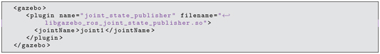
The wheel rotation values are published on joint_states because the URDF model contains the Gazebo option: publishWheelJointState true /publishWheelJointState . However, the joint_states topic does not contain other angles, including the caster wheel angles nor the arm joint angle (joint1).
The caster wheel angles are known to Gazebo, and these joint angles can be published to a ROS topic by including another Gazebo plug-in in the model. The model file mobot_w_jnt_pub.xacro (in the mobot_urdf package) is the same as mobot2.xacro, except for the addition of the following lines:
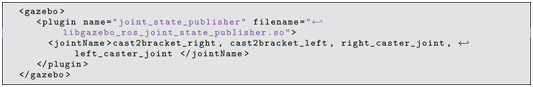
libgazebo_ros_joint_state_publisher.so This Gazebo plug-in accesses the internal Gazebo dynamic model to obtain the joint values for the named joints, and it publishes these values to the joint_states topic.
Similarly, the model file minimal_robot_w_jnt_pub.urdf in the minimal_robot_description package is identical to minimal_robot_description_unglued.urdf, except for the addition of the following lines:
which invokes the libgazebo_ros_joint_state_publisher.so Gazebo plug-in to publish the values of joint1 angles to the joint_states topic.
These two modified files are included in a common model file, mobot_w_arm_and_jnt_pub.xacro (in the mobot_urdf package), as follows:

Listing 4.1 mobot_w_arm_and_jnt_pub.xacro
The mobot_w_arm_and_jnt_pub.xacro model file is identical to mobot_w_arm.xacro, except that it includes the modified mobot and arm model files. The mobot_w_arm_and_jnt_pub.xacro model file is referenced in a launch file, mobot_w_arm_and_jnt_pub.launch:
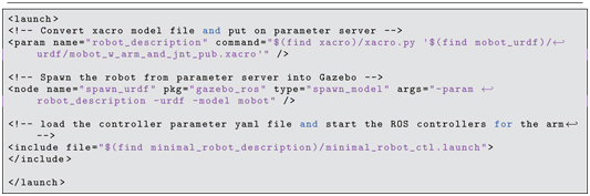
Listing 4.2 mobot_w_arm_and_jnt_pub.launch
To observe the effects of the joint-state publisher Gazebo plug-in, kill and restart Gazebo:

and then invoke the new launch file:

This again brings up the mobile robot with attached one-DOF arm. Now, however, the joint_states topic is richer. Example output of:

(excerpted) is:

We see that now there are seven joint values being published. These values are needed to compute transforms for link poses. Given the model description, which prescribes how connected links relate to each other through joint displacements, it is possible to compute all individual transforms for pair-wise connected links. This could be done manually from the information available. However, this is such a common need that ROS has a package designed to do this: the robot_state_publisher (see http://www.w3.org/1999/xlink). robot_state_publisher
With the simulation running, invoking:

results in the tf topic being much richer as well. Excerpts from the output of:

follow:
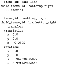
From the tf output, one can follow chains of transforms. One kinematic branch starts at base_link and has successive parent-child connections through castdrop_right (a static transform) to brackettop_right (which swivels about its z axis, as evidenced by the quaternion values), to bracketside1_right (a static transform) to right_casterwheel (which spins about its axle). The individual transforms can be multiplied together (an operation defined in the transform class, equivalent to multiplying matrices) to find the pose of any link frame with respect to any desired reference frame (as long as there is a complete chain between the two frames).
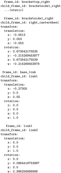
Note also the transform between base_frame and link1 (a static transform) and the transform between link1 and link2 (which depends on the joint1 angle). From these transforms, one can obtain the frame of link2 of the one-DOF robot with respect to the base link. ROS also provides facilities to compute transforms between any two (connected) frames within a user’s program with a transform_listener, details of which are introduced in Section 4.2.
4.2 Transform listener
Performing transforms from one frame to another is enabled by the tf library transform listener in ROS (see: http://www.w3.org/1999/xlink). A very useful capability in the tf library is the tf_listener. We have seen that transforms are published to the topic tf, where each such message contains a detailed description of how a child frame is spatially related to its parent frame. (In ROS, a parent can have multiple children, but a child must have a unique parent, thus guaranteeing a tree of geometric relationships.) The tf_listener is typically started as an independent thread (thus not dependent on spin() or spinOnce() invocations from a main program). This thread subscribes to the tf topic and assembles a kinematic tree from individual parent-child transform messages. Since the tf_listener incorporates all transform publications, it is able to address specific queries, such as “where is my right-hand palm frame relative to my left-camera optical frame?” The response to such a query is a transform message that can be used to reconcile different frames (e.g. for hand-eye coordination). As long as a complete tree is published connecting frames of interest, the transform listener can be used to transform all sensor data into a common reference frame, thus allowing for display of sensory data from multiple sources in a common view.
Use of the tf listener is illustrated with example code in the package example_tf_listener of the accompanying code repository. This illustrative package specifically assumes reference to our mobot model, notably with respect to frames base_link, link1 and link2. The example code is comprised of three files: example_tf_listener.h, which defines a class DemoTfListener; example_tf_listener_fncs.cpp, which contains the implementation of the class methods of DemoTfListener; and example_tf_listener.cpp, which contains a main() program illustrating operations using a transform listener. The contents of the main program are shown in Listing 4.3.
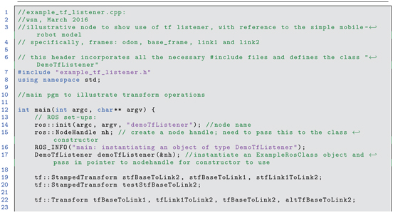
Listing 4.3 example_tf_listener.cpp: example code illustrating transform listener
In Listing 4.3, an object of class DemoTfListener is instantiated (line 17). This object has a transform listener, a pointer to which is tf::TransformListener* tfListener_;. The transform listener is used in four places in the main program: lines 24, 29, 34 and 57. tf::TransformListener transformPose() lookupTransform()
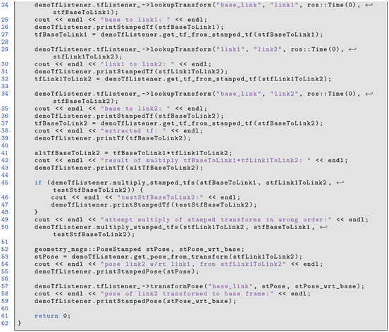
The first instance, line 24, is:

The transform listener subscribes to the tf topic and it constantly attempts to assemble the most current chain of transforms possible from all published parent-child spatial relationships. The transform listener, once it has been instantiated and given a brief time to start collecting published transform information, offers a variety of useful methods. In the above case, the method lookupTransform finds a transformation between the named frames (base_link and link1). Equivalently, this transform tells us where is the link1 frame with respect to the base_link frame. The lookupTransform method fills in stfBaseToLink1, which is an object of type tf::StampedTransform. A stamped transform contains both an origin (a 3-D vector) and an orientation(a matrix). The example code prints components of this transform, using accessor functions of transform objects. tf::StampedTransform
The lookupTransform() function is called with arguments to define the frame of interest (link1) and the desired reference frame (base_link). The argument ros::Time(0) specifies that the current transform is desired. (Optionally, one can request a transform a historical transform corresponding to some specified time of interest in the past.) ros::Time(0)
The object stfBaseToLink1 has a timestamp, labels for the reference frame (frame_id) and for the child frame (child_frame_id), and a tf::Transform object. Objects of type tf::Transform frame_id child_frame_id have a variety of member methods and defined operators. Extracting the tf::Transform from a tf::StampedTransform object is not as simple as would be expected. The function get_tf_from_stamped_tf() is defined within the class DemoTfListener to assist. On line 27,

the tfBaseToLink1 transform is extracted from stfBaseToLink1. This transform describes the position and orientation of frame link1 with respect to frame base_frame.
On line 29, the stamped-transform stfLink1ToLink2 is obtained using the transform listener, but with specified frame of interest link2 with respect to frame link1. The transform is extracted from the stamped transform into the object tfLink1ToLink2.
Lines 34 and 37 perform this operation again, this time to populate tfBaseToLink2, which is the transform of link2 with respect to base_frame.
The operator is defined for tf::Transform objects. Thus, the objects tfBaseToLink1 and tfLink1ToLink2 can be multiplied together, as in line 41: tf::Transform, multiplication

The meaning of this operation is to cascade these transforms, equivalent to multiplying transforms:
7
The result in altTfBaseToLink2 is the same as the result of

and extracting the transform from stfBaseToLink2.
The example code displays the various transforms using the member functions printTf() and printStampedTf() of class DemoTfListener.
Line 57 shows use of another member method of the transform listener:

transformPose() With this function, one can transform an object of type geometry_msgs::PoseStamped. geometry_msgs::PoseStamped The position and orientation of this pose are expressed with respect to the named frame_id. With the transformPose() function, the input PoseStamped object, stPose, is re-expressed as an output pose, stPose_wrt_base, expressed with respect to the named, desired frame (base_link, in this example).
To see the results of the example code, start Gazebo with:

and invoke the mobot launch file:

Running:

one can see published transforms that include relationships among odom, base_link, left_wheel and right_wheel, which are published courtesy of the differential-drive Gazebo plug-in. To get more transforms, including the minimal robot arm, run:

robot_state_publisher The tf topic then carries many additional transform messages, including link2 to link1 (of the minimal robot arm) and link1 to base_link.
With these nodes running, start the example transform listener:

The example transform listener output begins with:

Initially, the transform listener does not have knowledge of all of the incremental transforms of the kinematic tree. The transform listener call thus fails. This failure is trapped, and the call is re-attempted. By the time of the next try, the connecting transforms are all known and the call is successful. Ordinarily, successive attempts to find transforms between any two named frames will be successful. However, it is still good practice to use “try and catch” in case of future missing transforms. tf, try/catch
The first result displayed is:
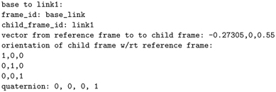
This shows that the transform between frame base_link and frame link1 is relatively simple. The orientation is merely the identity, indicating that the link1 frame is aligned with the base_link frame. The vector from the base_link frame origin to the link1 frame origin has a negative x component, a 0 y component and a positive z component. This makes intuitive sense, as the link1 frame origin is above the base_link origin (and thus positive z component) and behind the base_link frame origin (and thus the negative x component). The quaternion corresponding to the identity matrix orientation is (0,0,0,1).
The next part of the display output is:
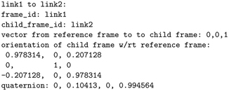
The vector from the link1 frame origin to the link2 frame origin, (0, 0, 1), is simply a 1 m displacement in the z direction. The link2 frame is nearly aligned with the link1 frame. The y axis (second column of the rotation matrix) is (0,1,0), which implies the link2 y axis is identically parallel to the link1 y axis. However, the x and z axes of the link2 frame are not identical to the corresponding link1 axes. Since link2 is leaning slightly forward, the link2 z axis, (0.207, 0, 0.078), has a slight positive x component (as expressed with respect to the link1 frame), and the link2 x axis, , points slightly down, and thus has a negative z component (with respect to the link1 frame). The next display output corresponds to the transform between link2 and the base link.

For comparison, the output of the product tfBaseToLink1 and tfLink1ToLink2 is:
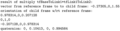
The components of this result are identical to those of the transform lookup directly from the base link to link2, demonstrating that products of transforms behave equivalent to matrix transform multiplications (although the result of tf::Transform multiplications are objects of type tf::Transform, not merely matrices).
Multiplication of tf::StampedTransform objects is not defined. However, a member function of class DemoTfListener performs the equivalent operation. Line 45:

performs the expected operation. The transform components of the stamped transforms are extracted, multiplied together, and used to populate the transform component of a resulting stamped transform, testStfBaseToLink2. The example function gets assigned the frame_id of the first stamped transform and the child_id of the second stamped transform. However, for the multiplication to make sense, the child_id of the first stamped transform must be identical to the frame_id of the second stamped transform. If this condition is not satisfied, the multiplication function returns false to indicate a logic error. (See line 50.)
Finally, lines 52 through 59 illustrate how to transform a pose to a new frame. The output display is:
pose link2 w/rt link1, from stfLink1ToLink2
frame id = link1
origin: 0, 0, 1
quaternion: 0, 0.10413, 0, 0.994564
pose of link2 transformed to base frame:
frame id = base_link
origin: -0.27305, 0, 1.55
quaternion: 0, 0.10413, 0, 0.994564
Note that the transformed link2 pose has a translation and a rotation identical to the corresponding components of the stamped transform stfBaseToLink2 obtained using tfListener_- lookupTransform.
Another check on this transform can be obtained with use of a command-line tool within the tf package. Running:

tf tf_echo results in output to the screen displaying the transform between the named frames. The order of naming matters. The above command displays the frame of link2 with respect to frame base_link. Example output from this command is:

which agrees with the transform-listener result.
Converting between geometry_msgs types and tf types can be tedious. The code in Listing 4.4, extracted from example_tf_listener_fncs.cpp, illustrates how to extract a geometry_msgs::PoseStamped from a tf::StampedTransform.
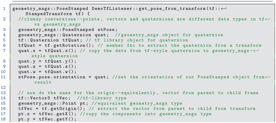

Listing 4.4 example conversion from tf to geometry_msgs type
Although vectors and quaternions are defined within geometry_msgs and tf, these types are not compatible. The code in Listing 4.4 shows how these can be converted.tf and geometry_msgs type conversions
When instantiating a transform listener, it was noted that the lookup function should be tested for return errors. This is done in the constructor of DemoTfListener, as shown in Listing 4.5, extracted from example_tf_listener_fncs.cpp.
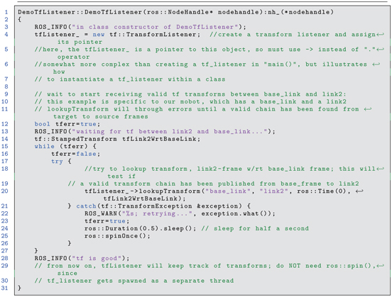
Listing 4.5 constructor of DemoTfListener illustrating tfListener
The try and catch construct is used to trap errors from the lookupTransform() function of the transform listener. When using a transform-listener lookup function, it is advisable to always have a try and catch test. Otherwise, if the lookup function fails, the main program will crash. lookupTransform()
Another concern with the transform listener is clock synchronization of multiple computers running nodes within a common ROS system. ROS supports distributed processing. However, with a network of computers, each computer has its own clock. This can cause time stamps within published transforms to be out of synchronization. The transform listener may complain that some transforms appear to be posted for times in the future. Resolution of this problem may require using chrony (see http://www.w3.org/1999/xlink) or some alternative network time protocol clock synchronization. time synchronization chrony
Additional functions in example_tf_listener_fncs.cpp include multiply_stamped_tfs(), get_tf_from_stamped_tf(), get_pose_from_transform(), printTf(),printStampedTf() and printStampedPose(). These will not be covered in detail here, but viewing the source code can be useful in understanding how to access or populate components of transform types. The conversions introduced here are incorporated within a useful library called XformUtils, which will be described in the next section. In addition to tf operations, an alternative library known as Eigen can be more convenient for performing linear-algebra operations, as introduced next.
4.3 Using Eigen library
ROS messages are designed for efficient serialization for network communication. These messages can be inconvenient to work with when one desires to perform operations on data. One common need is to perform linear algebra operations. A useful C++ library for linear algebra is the Eigen library (see http://www.w3.org/1999/xlink). The Eigen open-source project is independent of ROS. However, one can still use Eigen with ROS. Eigen library
To use Eigen with ROS, one must include the associated header files in the *.cpp source code and add lines to CmakeLists.txt. Our custom cs_create_pkg script already includes the necessary lines in CmakeLists.txt; they only need to be uncommented. Specifically, uncomment the following lines in the CMakeLists.txt file: Eigen and CMakeLists.txt

(see http://www.w3.org/1999/xlink for an explanation of cmake_modules in ROS). In the source code, include the header files for the functionality desired. The following steps include much functionality:

For access to additional capabilities in Eigen, more header files may be included, as described in http://www.w3.org/1999/xlink.
A program that illustrates some Eigen capabilities is example_eigen_plane_fit.cpp in the package example_eigen. Lines from this program are explained here.
An example vector may be defined as follows:

This instantiates an Eigen object that is a column vector comprised of three double-precision values. The object is named normal_vec, initialized to the values [1;2;3].
One of the member functions of Eigen::Vector3d is norm(), which computes the Euclidean length of the vector (square root of the sum of squares of the components). The vector can be coerced to unit length (if it is a non-zero vector!) as follows: Eigen::Vector3d

Note that, although normal_vec is an object, the operators and / are defined to scale the components of the vector as expected. Thus, vector-times-scalar operations behave as expected (where normal_vec.norm() returns a scalar value).
Here is an example of instantiating a matrix object comprised of double-precision values:

With the following notation, one can fill the matrix with data, one row at a time:

There are a variety of other methods for initializing or populating matrices and vectors. For example, one can fill a vector or matrix with zeros using:
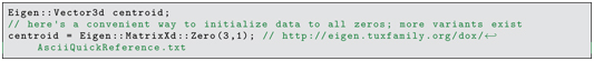
The arguments (3,1) specify 3 rows, 1 column. (A vector is simply a special case of a matrix, for which there is either a single row or a single column.)
Alternatively, one may specify initial values as arguments to the constructor upon instantiation. To initialize a vector to values of 1:

Eigen::MatrixXd
In the illustrative example code, a set of points is generated that lie on (or near) a pre-determined plane. Eigen methods are invoked to discover what was the original plane, using only the data points. This operation is valuable in point-cloud processing, where we may wish to find flat surfaces of interest, e.g. tables, walls, floors, doors, etc.
In the example code, the plane of interest is defined to have a surface normal called normal_vec, and the plane is offset from the origin by a distance dist. A plane has a unique definition of distance from the origin. If one cares about positive and negative surfaces of a plane, the distance from the origin can be a signed number, where the offset is measured from origin to plane in the direction of the plane’s normal (and thus can result in a negative offset).
To generate sample data, we construct a pair of vectors perpendicular to the plane’s normal vector. We can do so starting with vector v1 that is not colinear with the plane normal. In the example code, this vector is generated by rotating normal_vec 90 degrees about the z axis, which is accomplished with the following matrix*vector multiply:

(Note: if normal_vec is parallel to the z axis, v1 will be equal to normal_vec, and the subsequent operations will not work.)
For display purposes, Eigen types are nicely formatted for cout. Matrices are formatted with new lines for each row, e.g. using:

Rather than use cout, it is preferable to use ROS_INFO_STREAM(), which is more versatile than ROS_INFO(). This function outputs the data via network communication, and it is thus visible via rqt_console and loggable. To display Rot_z as a formatted matrix with ROS_INFO_STREAM(), one can use: ROS_INFO_STREAM()

For short column vectors, it is more convenient to display the values on a single line. To do so, one can output the transpose of the vector, e.g. as follows:

Two common vector operations are the dot product and the cross product. From the example code, here are some excerpts:

and for the cross product, v1 crossed into normal_vec:
Eigen, dot product Eigen, cross product

Note that the result of v1 x normal_vec must be mutually orthogonal to both v1 and normal_vec. Since the result, v2, is perpendicular to normal_vec, it is parallel to the plane under construction.
A second vector in the plane can be computed as:

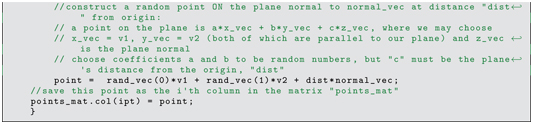
Using the vectors v1, v2 and normal_vec, one can define any point in the desired plane as:

with the constraint c = dist, but a and b can be any scalar values.
Random points in the plane are generated and stored as column vectors in a matrix. The matrix is instantiated with the line:

The example generates random points within the desired plane as follows:
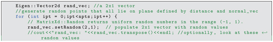
Random noise can be added to the (ideal) data on the plane using:
Random noise can be added to the (ideal) data on the plane using:

The matrix points_mat now contains points, column by column, that approximately lie on a plane distance dist from the origin and with surface-normal vector normal_vec. This dataset can be used to illustrate the operation of plane fitting. The first step is to compute the centroid of all of the points, which can be computed as follows:

The (approximately) planar points are then offset by subtracting the centroid from each point.

The resulting matrix (three rows and npts columns) can be used to compute a covariance matrix by multiplying this matrix times its transpose, resulting in a matrix:

One of the more advanced Eigen options is computation of eigenvectors and associated eigenvalues. This can be invoked with:
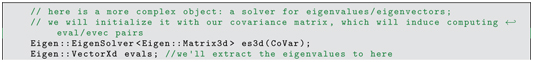

Eigen::EigenSolver The three eigenvalues are all non-negative. The smallest of the eigenvalues corresponds to the eigenvector that is the best-fit approximation to the plane normal. (The direction of smallest variance is perpendicular to the best-fit plane.) If the smallest eigenvalue corresponds to index ivec, the corresponding eigenvector is:

The distance of the plane from the origin can computed as the projection (dot product) of the vector from the origin to the centroid onto the plane normal:

The program example_eigen_plane_fit.cpp illustrates a variety of Eigen capabilities, and the specific algorithm illustrated is an efficient and robust technique for fitting planes to data.
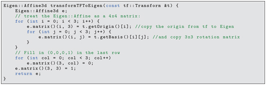
Another Eigen object that will be useful is Eigen::Affine3d, which has the equivalent capabilities of a coordinate-transform operator. Eigen::Affine3d A ROS tf transform can be converted to an Eigen affine object as follows:
Subsequently, Eigen affine objects can be multiplied together, or premultiplied by Eigen Vector3d objects to transform points to new coordinates frames, as in the following example code snippet:
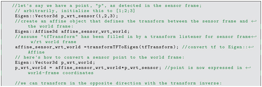

Eigen-style affine transforms are very useful both in computing poses of kinematic chains and transforming sensor data into useful reference frames, such as a robot’s base frame.
4.4 Transforming ROS datatypes
XformUtils transform conversions As we have seen, ROS nodes communicate with each other through defined message types. A ROS publisher deconstructs the data components of a message object, serializes the data and transmits it via a topic. A complementary subscriber receives the serial data and reconstructs the components of the corresponding message object. This process is convenient for communications, but message types can be cumbersome for performing mathematical operations. For example, a geometry_msgs::Pose object can be inspected in terms of its individual elements, but it cannot be used directly in linear algebraic operations.
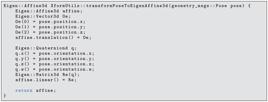
The package xform_utils contains a library of convenient conversion functions. For example, transformPoseToEigenAffine3d(), which takes a geometry_msgs::Pose and returns an equivalent Eigen::Affine3d, is given below.
To use these utility functions in one’s own package, the package should include xform_utils dependency in package.xml, and the package source code should include the header file #include xform_utils/xform_utils.h . Within the source code, an object of type XformUtils can be instantiated, after which the member functions can be used.
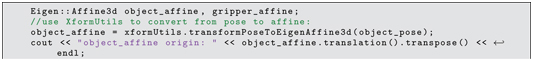
Example usage is illustrated in the source code example_xform_utils.cpp in the xform_utils package. This example anticipates a forthcoming need to transform from an object pose to a gripper pose. In this instance, the object pose is hard coded, with position and orientation components of a geometry_msgs::Pose object called object_pose. A gripper approach pose is to be derived in which the origin of the gripper frame is identical to the origin of the object frame, the x axis of the gripper frame is coincident with the object frame, and the z axis of the gripper frame is anti-parallel to the z axis of the object frame. This is constructed as follows. Given the populated object frame, it is transformed into an equivalent Eigen::Affine3d object using XformUtils, and the components of the affine are displayed:

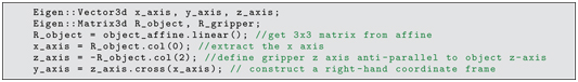
The rotation matrix of the Affine3d object is interpreted in terms of x, y and z direction axes. These are used to construct the corresponding axes of the gripper frame. The x axis of the gripper frame is identical to the x axis of the object frame, and the z axis of the gripper frame is the negative of the z axis of the gripper frame. The y axis is constructed as the cross product of z into x to create a right-hand triad.
From the object origin and the constructed orientation, the gripper affine is populated:

The resulting Affine3d object is converted into a pose (using a XformUtils function), and this pose is used in populating a PoseStamped object, and the result is displayed (using another XformUtils function).

This illustrates how object types in ROS can be transformed to be compatible with additional libraries (notably, the Eigen library) to exploit additional library functions. The specific example used here will be useful in computing poses for manipulation, as discussed in Section .
4.5 Wrap-Up
Coordinate transforms are ubiquitous in robotics, and correspondingly, ROS has extensive tools for handling coordinate transforms. These can be somewhat confusing, though, since there are multiple representations. The tf library offers a tf listener that can be used conveniently within nodes to listen for all transform publications and assemble these into coherent chains. The tf listener can be queried for spatial relationships between any two connected frames. The listener responds with the most current transform information available. In contrast, a planner would consider hypothetical relationships. As such, tf is less useful for planning purposes, and thus one may need to compute kinematic transforms independently for planning. Additionally, although tf is updated dynamically, a potential limitation is that the assembled chains of transforms may be slightly time delayed. Consequently,tf results should not be used in time-critical feedback loops (e.g. for force control, for which it may be necessary to compute one’s own kinematic transforms).
The Eigen library, which is independent of ROS, can be integrated within ROS nodes to perform fast and sophisticated linear algebra computations. Eigen transforms can use matrices or the Eigen datatype Eigen::Affine3. As with other independent libraries, conversions are required between ROS message types and (in this case) Eigen objects. Such conversions require some extra overhead, but the benefits are worth the effort.
With an understanding of transforms in ROS, we are ready to introduce the valuable ROS visualization tool known as rviz.