CHAPTER 8
Point Cloud Processing
CONTENTS
8.1 Simple point-cloud display node
8.2 Loading and displaying point-cloud images from disk
8.3 Saving published point-cloud images to disk
8.4 Interpreting point-cloud images with PCL methods
INTRODUCTION
Interpreting 3-D sensory data is enabled with the use of the Point Cloud Library Point Cloud Library Point Cloud Processing (see http://www.w3.org/1999/xlink). This open-source effort is independent of but compatible with ROS. The Point Cloud Library (PCL) offers an array of functions for interpreting 3-D data. The present treatment is not intended to be a comprehensive tutorial of PCL. Rather, a few simple capabilities are introduced that provide useful functionality. Greater expertise can be gained by consulting the on-line tutorials and code examples. (At the time of this writing, there appears to be no textbook for teaching PCL.) It is hoped that the incremental examples discussed here will help to make the on-line resources more accessible.
8.1 Simple point-cloud display node
The pclutils package contains the source program displayellipse.cpp and the associated module makeclouds.cpp. This program introduces use of some basic PCL datatypes and conversions to ROS-compatible messages. This package was created using cscreatepkg with options of roscpp, sensormsgs, pclros and pclconversions. (Additional dependencies of stdmsgs and tf are used in later examples.)
Within the displayellipse node, a point-cloud object is populated with computed values that describe an ellipse extruded in the z direction that has coloration that varies in the z direction.
The source code of the function that populates a point cloud is shown in Listing 8.1.
Listing 8.1 make_clouds.cpp: C++ code illustrating populating a point cloud
The function makeclouds() accepts pointers to PCL PointCloud objects and fills these objects with computed data. The object pcl::PointCloud pcl::PointXYZ is templated to accommodate different types of point clouds. We specifically consider basic point clouds (type pcl::PointXYZ), which have no color associated with individual points, and colored point clouds (type pcl::PointXYZRGB).
A PCL point-cloud object contains fields for a header, which includes a field for frameid, and components that define the height and width of the point cloud data. Point clouds can be unordered or ordered. In the former case, the point-cloud width will be the number of points, and the point-cloud height will be 1. An unordered point cloud is a “bucket of points” in no particular order. PointCloud object
The first argument of this function is a pointer to a simple point cloud, consisting of (x, y, z) points with no associated intensity or color. The second argument is a pointer to an object of type pcl::PointXYZRGB, which will be populated with points that have color as well as 3-D coordinates. PCL pcl::PointXYZRGB PCL pcl::PointXYZ
Lines 28 and 29 instantiate variables of type pcl::PointXYZ and pcl::PointXYZRGB, which are consistent with elements within corresponding point clouds. An outer loop, starting on line 31, steps through values of z coordinates. At each elevation of z, coordinates x and y are computed corresponding to an ellipse. Lines 47 through 49 compute these points and assign them to elements of the basicpoint object:

On line 50, this point is appended to the vector of points within the uncolored point cloud:

In lines 53 through 55, these same coordinates are assigned to the colored point object. The associated color is added on line 57:

and the colored point is added to the colored point cloud (line 58):

Encoding of color is somewhat complex. The red, green and blue intensities are represented as values from 0 to 255 in unsigned short (eight-bit) integers (line 25). Somewhat awkwardly, these are encoded as three bytes within a four-byte, single-precision float (lines 37 through 41).
At each increment of z value, the R, G and B values are altered (lines 60 through 67) to smoothly change the color of points in each z plane of the extruded ellipse.
Lines 71 through 77 set some meta-data of the populated point clouds. The lines:

specify a height of 1, which implies that the point cloud does not have an associated mapping to a 2-D array and is considered an unordered point cloud. PointCloud, unordered Correspondingly, the width of the point cloud is equal to the total number of points.
When the makeclouds() function concludes, the pointer arguments basiccloudptr and pointcloudptr point to cloud objects that are populated with data and header information and are suitable for analysis and display.
The displayellipse.cpp file, displayed in Listing 8.2 shows how save a point-cloud image to disk, as well as publish a point cloud to a topic consistent with visualization via rviz. This function instantiates point-cloud pointers (lines 24 through 25), which are used as arguments to the makeclouds() function (line 31).

Listing 8.2 display_ellipse.cpp: C++ code illustrating publishing a point cloud
On line 34, a PCL function is called to save the generated point cloud to disk:

PCL PCD files This instruction causes the point cloud to be saved to a file named ellipse.pcd (in the current directory, i.e. the directory from which this node is run).
For ROS compatibility, point-cloud data is published using the ROS message type sensormsgs/PointCloud2. This message type is suitable for serialization and publications, but it is not compatible with PCL operations. The packages pclros and pclconversions offer means to convert between ROS point-cloud message types and PCL point-cloud objects. pcl_ros pcl_conversions
The PCL-style point cloud is converted to a ROS-style point-cloud message suitable for publication (lines 36 and 37). The ROS message roscloud is then published (line 46) on topic ellipse (as specified on line 41, upon construction of the publisher object).
To compile the example program, the CMakeLists.txt file must be edited to reference the point-cloud library. Specifically, the lines:

are uncommented in the provided CMakeLists.txt auto-generated file. This change is sufficient to bring in the PCL library and link this library with the main program.
With a roscore running, the example program can be started with

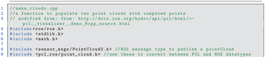
This node has little output, except to remind the user to select topic ellipse and frame camera to view the point-cloud publication in rviz. Starting rviz and selecting camera as the fixed frame and selecting ellipse for the topic in a PointCloud2 display yields the result in Fig 8.1.
Figure 8.1 Rviz view of point cloud generated and published by display_ellipse.
As expected, the image consists of sample points of an extruded ellipse with color variation in the extrusion (z) direction. This image can be rotated, translated and zoomed in rviz, which helps one to perceive its 3-D spatial properties.
The function savePCDFileASCII invoked on line 34 PCL, savePCDFileASCII PCL, savePCDFile causes the file to be saved in ASCII format, whereas an alternative command savePCDFile would save the point cloud in binary format. The ASCII representation should be used sparingly. ASCII files are typically more than twice the size of binary files. Further, there is (currently) a bug in the ASCII storage that results in some color corruption. Nonetheless, the ASCII option can be useful for understanding PCD file formats.
The ASCII file ellipse.pcd can be viewed with a simple text editor. The beginning of this file is:

The file format contains metadata describing how the point cloud is encoded, followed by the data itself. (Details of the file format can be found at http://www.w3.org/1999/xlink.) The field names, in order, are x y z rgb. The WIDTH of the data is 2920, which is identical to the POINTS. The HEIGHT is simply 1, and WIDTH HEIGHT = POINTS. This description means that the point cloud is stored merely as a list of points–an unordered point cloud–without any inherent structure (or at least none that is encoded in the file).
Following the description of how the data is encoded, the actual data is listed. Only six lines of this data are shown; the entire data includes 2920 points. As can be seen from the first six lines, all values of z are , which is consistent with the outer z-height loop of makeclouds() (which starts at ). The x and y values are also consistent with the sin and cos values expected. The fourth value is harder to interpret, since the RGB data is encoded as three of four bytes in the single-precision floating-point value.
In the next section, we will see the alternative of an ordered point-cloud encoding.
8.2 Loading and displaying point-cloud images from disk
In the previous section, a point cloud was populated with computed data. More typically, one would be working with point-cloud data acquired by some form of depth camera, e.g. a depth camera such as the Kinect™, a scanning LIDAR such as the Carnegie Robotics sensor head, or point clouds generated by stereo vision. Such data is typically acquired and processed online during robot operation, but it is also convenient to save snapshots of such data to disk, e.g. for use in code development or creation of an image database.
A simple example of reading a PCD file from disk and displaying it to rviz is provided in displaypcdfile.cpp, which is shown in Listing 8.3. PCD file display

Listing 8.3 display_pcd_file.cpp C++ code illustrating reading PCD file from disk and publishing it as a point cloud
Lines 37 through 48 of Listing 8.3 are equivalent to corresponding lines in the previous displayellipse program. The topic is changed to pcd (line 37) and the frameid is set to cameradepthopticalframe (line 40), and these must be set correspondingly in rviz to view the output. camera_depth_optical_frame
The primary difference with this example code is that the user is prompted to enter a file name (lines 23 through 25), and this file name is used to load a PCD file from disk and populate the pointer pclclrptr (line 27):

As a diagnostic, lines 32 through 34 inspect the width and height fields of the opened point cloud, multiply these together, and print the result as the number of points in the point cloud.
Example PCD files reside in the accompanying repository within the ROS package pcdimages. A snippet of an example PCD file from a Kinect camera image, stored as ASCII, is:

This example is similar to the ellipse PCD file, with the notable exception that the HEIGHT parameter is not unity. The HEIGHT WIDTH is , which is the sensor resolution of the Kinect color camera. The total number of points is 307,200, which is . In this case, the data is an ordered point cloud, since the listing of point data corresponds to a rectangular array. PointCloud, ordered
An ordered point cloud preserves potentially valuable spatial relationships among the individual 3-D points. A Kinect camera, for example, has each 3-D point associated with a corresponding pixel in a 2-D (color) image array. Ideally, an inverse mapping also associates each pixel in the 2-D array with a corresponding 3-D point. In practice, there are many “holes” in this mapping for which no valid 3-D point is associated with a 2-D pixel. Such missing data is represented with NaN (not-a-number) codes, as is the case with the initial point values in the PCD file snippet shown above.
Coordinate data within a point-cloud object typically is stored as four-byte, single-precision floating-point values. Single-point precision is more than adequate for the level of precision of current 3-D sensors, and thus this lower-precision representation helps reduce file size without compromising precision.
Running the display node with

prompts the user to enter a file name. If the node is run from the pcdimages directory, the file name entered will not require a directory path. Entering the file name cokecan.pcd results in the response:

which is the number of points expected for a Kinect-1 image. In rviz, setting the topic to pcd and setting the fixed frame to cameradepthopticalframe produces the display shown in Fig 8.2.
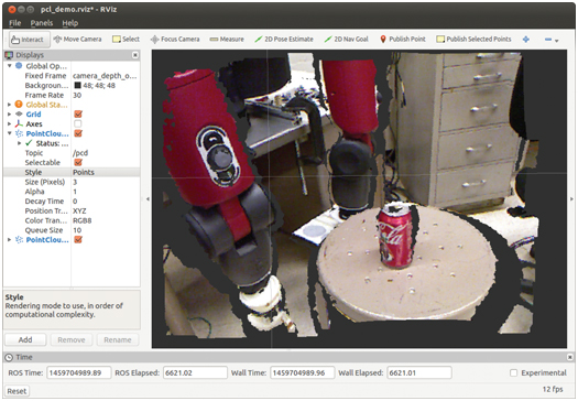
Figure 8.2 Rviz view of image read from disk and published by display_pcd_file.
8.3 Saving published point-cloud images to disk
A convenient utility program in the pclutils package is pcdsnapshot.cpp. The contents of this program are shown in Listing 8.4. pcl_utils snapshot
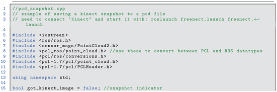

Listing 8.4 pcd_snapshot.cpp C++ code illustrating subscribing to point-cloud topic and saving data to disk as PCD file
In this program, a ROS subscriber subscribes to topic camera/depthregistered/points (line 30) with a callback function, kinectCB(), listening for messages of type sensormsgs/PointCloud2 (lines 18 through 25). When a message is received by the callback function, it converts the message to a pcl::PointCloud type (line 21). The callback function signals that it has received a new image by setting gotkinectimage to “true.”
The main program waits for the gotkinectimage signal (line 34), and upon confirmation, the main program saves the acquired image as filename kinectsnapshot.pcd within the current directory (line 40):

To use this program with a Kinect camera, plug in the camera, and with a roscore running, start the Kinect driver:

(If the freenect driver is not already installed on your system, it will need to be installed. This installation is included with the provided setup scripts.)
Start rviz, and set the fixed frame to cameradepthopticalframe, add a PointCloud2 item and set its topic to camera/depthregistered/points. This will provide a real-time view of the Kinect data, published as a ROS point cloud. rviz, displaying Kinect data
To prepare to capture an image, open a terminal and navigate to a directory relevant for storing the image. When the rviz display shows a scene to be captured, run the node:

This will capture a single point-cloud transmission and save the captured image to disk (in the current directory) as a PCD file called kinectsnapshot.pcd. The saved image will be in binary format, and it will store the colored, ordered point cloud. To take more snapshots, re-name kinectsnapshot.pcd to something mnemonic, and re-run pcdsnapshot. (If you do not re-name the previous snapshot, the file kinectsnapshot.pcd will be overwritten.)
The image in Fig 8.2 was acquired in this manner. The resulting PCD file can be read from disk and displayed, using displaypcdfile, or it can be read into another application to perform interpretation of the point-cloud data.
8.4 Interpreting point-cloud images with PCL methods
Within the pclutils package, the program findplanepcdfile.cpp (displayed in Listing 8.5) illustrates use of a few PCL methods. The functions are illustrated operating on a PCD file. Lines 56 through 65 are similar to displaypcdfile, in which the user is prompted for a PCD file name, which is then read from disk. The resulting point cloud is published on topic “pcd” (lines 68, 73 and 108), making it viewable via rviz.


Listing 8.5 find_plane_pcd_file.cpp C++ code illustrating use of PCL methods
A new feature introduced in this program, voxel filtering, appears in lines 78 through 81:
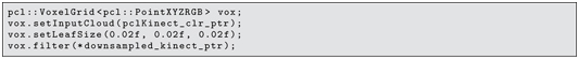
pcl::VoxelGrid These instructions instantiate a PCL-library object of type VoxelGrid that operates on data of type pcl::PointXYZRGB (colored point clouds). The VoxelGrid object, vox, has member functions that perform spatial filtering for down-sampling. (For greater detail, see http://www.w3.org/1999/xlink.) Typical of PCL methods, the first operation with vox is to associate point-cloud data with it (on which the object will operate). PCL attempts to avoid PCL, down-sampling making copies of data, since point-cloud data can be voluminous. Pointers or reference variables are typically used to direct the methods to the data already in memory. After affiliating vox with the point cloud read from disk, parameters are set for leaf size. The x, y and z values have all been set to 0.02 (corresponding to a 2 cm cube).
With the instruction filter, the vox object filters the input data and produces a down-sampled output (which is populated in a cloud via the pointer downsampledkinectptr). Conceptually, down-sampling by this method is equivalent to subdividing a volume into small cubes and assigning each point of the original point cloud to a single cube. After all points are assigned, each non-empty cube is represented by a single point, which is the average of all points assigned to that cube. Depending on the size of the cubes, the data reduction can be dramatic, while the loss of resolution may be acceptable.
In the example code, lines 86 and 110 convert the down-sampled cloud to a ROS message and publish the new cloud to the topic downsampledpcd. The sizes of the original and down-sampled clouds are printed out (lines 84 and 85).
Running rosrun pclutils findplanepcdfile prompts for a file name. Using the same file as in Fig 8.2 (cokecan.pcd), downsampling at the chosen resolution (2cm cubes) results in printed output:
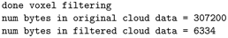
showing that down-sampling reduced the number of points by nearly a factor of 50 (in this case). Bringing up rviz, and setting the fixed frame to cameradepthopticalframe and choosing the topic downsampledpcd in a PointCloud2 display item produces the display in Fig 8.3. In this example, the severity of the downsampling is obvious, yet the image is still recognizable as corresponding to Fig 8.2. With the data reduction, algorithms applied to point-cloud interpretation can run significantly faster. (The choice of downsampling resolution would need to be tuned for any specific application).

Figure 8.3 Rviz view of image read from disk, down-sampled and published by find_plane_pcd_file.
In addition to demonstrating downsampling, the findplanepcdfile illustrates a means of interacting with the point-cloud data to assist interpretation of the data. The example code is linked with an example library that contains additional point-cloud processing examples, pclutils.cpp (in the pclutils package). This library defines a class, PclUtils, an object of which is instantiated on line 88. In addition, this object is shared with external functions via a global pointer, which is defined on line 35 and assigned to point to the PclUtils object on line 89.
One of the features of PclUtils is a subscriber that subscribes to the topic selectedpoints. The publisher on this topic is an rviz tool, publishselectedpoints, which allows a user to select points from an rviz display via click and drag of a mouse. The (selectable) points lying within the rectangle thus defined are published to the topic selectedpoints as a message type sensormsgs::PointCloud2. When the user selects a region with this tool, the corresponding (underlying) 3-D data points are published, which awakens a callback function that receives and stores the corresponding message.
Within findplanepcdfile, the value pclUtils.gotselectedpoints() is tested (line 94) to see whether the user selected a new patch of points. If so, a copy of the corresponding selected-points data is obtained (line 96) using the PclUtils method:

When a new copy of selected points is obtained, a function is called to analyze the down-sampled image in terms of a cue from the selected points (line 103):

PCL and rviz point selection
The function findindicesofplanefrompatch() is implemented in a separate module, findindicesofplanefrompatch.cpp, which resides in package pclutils. The contents of this module are shown in Listing 8.6.

Listing 8.6 find_indices_of_plane_from_patch.cpp C++ module showing PCL functions for interpretation of point-cloud data
The objective of this function is, given patchcloud points, which are presumably nearly coplanar, finding all other points in inputcloud that are nearly coplanar with the input patch. The result is returned in a vector of point indices, specifying which points in input cloud qualify as coplanar. This allows the operator to interactively select points displayed in rviz to induce the node to find all points coplanar with the selection. This may be useful e.g. for defining walls, doors, floor and table surfaces corresponding to the operator’s focus of attention. The example function illustrates use of PCL methods computePointNormal(), transformPointCloud(), and pcl::PassThrough filter methods setInputCloud(), setFilterFieldName(), setFilterLimits(), and filter(). pcl::PassThrough filter methods
On line 37 of findindicesofplanefrompatch(), the input cloud (a presumed nearly coplanar patch of points) is analyzed to find a least-squares fit of a plane to the points.

The fitted plane is described in terms of four parameters: the components (nx, ny, nz) of the plane’s surface normal, and the minimum distance of the plane from the camera’s origin (focal point). These parameters are returned in an Eigen-type vector via a the reference argument planeparameters. Additionally, the (scalar) curvature is returned in the curvature argument. The function computePointNormal() uses an eigenvalue-eigenvector approach to provide a robust best-estimate to a plane fit through the provided points. (See http://www.w3.org/1999/xlink for an explanation of the mathematical theory behind this implementation.)
When fitting a plane to points, there is an ambiguity regarding direction of the plane normal. The data alone cannot distinguish positive versus negative normal. Physically, solid objects have surfaces that distinguish inside from outside, and by convention the surface normal is defined to point toward the exterior of the object. PCL plane normal
In the current example, the point-cloud data is presumed to be expressed with respect to the camera’s viewpoint. Consequently, all points observable by the camera must correspond to surfaces that have a surface normal pointing (at least partially) toward the camera. When fitting a plane to points, if the computed surface normal has a positive z component, the normal vector must be negated to be logically consistent.
Additionally, the distance of a plane from a point (the focal point, in this case) is unambiguously defined. However, a signed distance is more useful, where the distance is defined as the displacement of the plane from the reference point along the plane’s normal. Since all surface normals must have a negative z component, all surfaces also must have a negative displacement from the camera-frame origin.
These corrections are applied as necessary within the function makeaffinefromplaneparams() (invoked on line 45). This function is a method within the pclutils library. The implementation of this method is displayed in Listing 8.7.
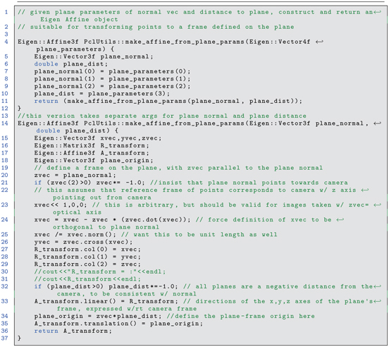
Listing 8.7 Method make_affine_from_plane_params() from Pcl_utils library
Lines 20 and 21 test and correct (as necessary) the surface normal of the provided patch of points. Similarly, line 32 assures that the signed distance of the plane from the camera’s origin is negative.
This function constructs a coordinate system on the plane defined by the plane parameters. The coordinate system has its z axis equal to the plane normal. The x and y axes are constructed (lines 23 through 26) to be mutually orthogonal and to form a right-hand coordinate system together with the z axis. These axes are used to populate the columns of a orientation matrix (lines 27 through 29), which constitutes the linear field of an Eigen::Affine object (line 33). The origin of the constructed coordinate system is defined to be the point on the plane closest to the camera-frame origin. This is computed as a displacement from the camera origin, in the direction opposite the plane normal, by (signed) distance equal to the plane-distance parameter (line 34). The resulting vector is stored as the translation() field of the Eigen::Affine object. The resulting populated affine object is returned.
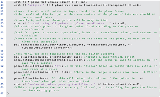
After function findindicesofplanefrompatch() calls function makeaffinefromplaneparams() (line 45 of Listing 8.6), the resulting affine is used to transform all of the input-cloud data. Noting that object Aplanewrtcamera specifies the origin and orientation of a coordinate frame defined on the plane, the input data can be transformed into the plane frame using the inverse of this affine object. A PCL function, transformPointCloud() can be used to transform a complete point cloud. This is invoked on line 57 of findindicesofplanefrompatch(), specifying the input cloud (*inputcloudptr), an object to hold the transformed cloud (*transformedcloudptr) and the desired transformation to apply to the input (Aplanewrtcamera.inverse()). PCL, transformPointCloud()

After being transformed into the coordinate frame defined on the plane, the data becomes easier to interpret. Ideally, all points coplanar with the plane’s coordinate frame will have a z component of zero. In dealing with noisy data, one must specify a tolerance to accept points that have nearly-zero z components. This is done using PCL filters in lines 60 through 64:
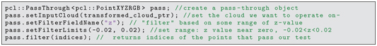
A PassThrough filter object is instantiated from the PCL library that operates on colored point clouds. This object is directed to operate on the point cloud specifed using the setInputCloud() method. The desired filter operation is specified by the setFilterFieldName() method, which in this case is set to accept (pass through) points based on inspection of their z coordinates. The setFilterLimits() method is called to specify the tolerance; here, points with z values between cm and 2 cm will be considered sufficiently close to zero. Finally, the method filter(indices) is called. This method performs the filtering operation. All points within the specified input cloud that have z values between and 0.02 are accepted, and these accepted points are identified in terms of their indices in the point data of the input cloud. These indices are returned within the vector of integer indices. The result is identification of points within the original point cloud that are (nearly) coplanar with the user’s selected patch. PCL, box filter
The calling function, the main program within findplanepcdfile given in Listing 8.5, invokes the function findindicesofplanefrompatch() (line 103) whenever the user selects a new set of points in rviz. This function returns with a list of points (in indices) that qualify as coplanar with the selected patch. Although these indices were selected from the transformed input cloud (expressed in the constructed plane’s frame), the same indices apply to the points in the original cloud (expressed with respect to the camera frame). The corresponding points are extracted from the original point cloud in line 104 using the PCL method copyPointCloud():

With this operation, the points referenced by index values in indices are copied from the down-sampled point cloud into a new cloud called planepts. This cloud is converted to a ROS message (line 106) and published (line 109) using a publisher object (line 69) defined to publish to topic planarpts.
By running the node findplanepcdfile on the same input file as before, points were selected from the rviz display as shown in Fig 8.4.
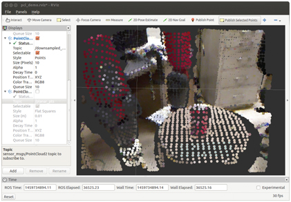
Figure 8.4 Scene with down-sampled point cloud and patch of selected points (in cyan).
A rectangle of points on the stool has been selected, as indicated by light cyan coloring of these points. The act of selecting points causes the findplanepcdfile node to compute a plane through the points, then find all points from the (down-sampled) point cloud that are (nearly) coplanar, and publish the corresponding cloud on topic planarpts.
Figure 8.5 shows the points chosen from the down-sampled point cloud that were determined to be coplanar with the selected patch.
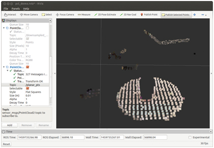
Figure 8.5 Points computed to be coplanar with selected points.
The points on the surface of the stool are correctly identified. However, additional points lie in the same plane, including points on the furniture and the robot in the background, that are not part of the surface of the stool. The selected points could be further filtered to limit consideration to x and y values as well (e.g., based on the computed centroid of the selected patch), thus limiting point extraction to only points on the surface of the stool. Points above the stool may also be extracted, yielding identification of points corresponding to objects on a surface of interest.
8.5 Object finder
PCL, object finder object_finder package The need for a robot to use vision for manipulation leads to introduction of another Kinect model. The simplekinectmodel2.xacro in package simplecameramodel contains a Kinect simulation with the camera pose similar to that which might be used by a robot, in this case elevated approximately 2 m from the floor and tilted looking downward, 1.2 rad from horizontal.
To provide an interesting scene for the camera, a world file has been defined in the worlds package, along with a complementary launch file. Running:

brings up Gazebo with a world model containing the DARPA Robotics Challenge starting pen, a cafe table, and a toy block.
After starting Gazebo with this world model, one can add the Kinect model with the launch file:

This launch file also brings up rviz with a saved settings file. The result of these two operations is shown in Fig 8.6.
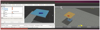
Figure 8.6 Scene of object on table viewed by Kinect camera.
The colors in rviz are not consistent with the colors in Gazebo, due to an inconsistency of how Gazebo and rviz encode colors. However, emulated cameras in Gazebo use the model colors as seen in Gazebo, so this is not an issue for development of vision code incorporating color. The block can be seen on the table in both the Gazebo model and in the Kinect data displayed in rviz. The camera model in the Gazebo scene is simply a white rectangular prism, apparently floating in space (since there is no visual model for a link supporting the camera).
From the Gazebo display, selecting the model toyblock, one can see that the block coordinates are , . The block model has a thickness of 0.035 m, and the block’s frame is in the middle of the prism.
A PCL processing node, objectfinderas, offers an action server that accepts an object code and attempts to find the coordinates of that object in the scene. Highlights of this action server are described in the following.
At the start of the main function, an object of the class ObjectFinder is instantiated:

This class is defined in the same file. It instantiates objectFinderActionServer. It also instantiates an object of the class PclUtils (from the package pclutils), which contains a collection of functions that operate on point clouds, as well as a subscriber to /kinect/depth/points, which receives publications of point clouds from the (simulated) Kinect camera.
Also within main(), the transform from the Kinect sensor frame to the world frame is found using a transform listener (line 233):

This transform is tested until it is successfully received, then the resulting transform is converted to an Eigen type:

This transform is subsequently used to transform all Kinect point-cloud points to express them with respect to the world frame. (It should be noted that achieving sufficient precision of this transform requires extrinsic calibration; see Section . In the present case with the simulator, the transform is known unrealistically precisely.) extrinsic camera calibration
Once main() has completed these initialization steps, the action-server waits for goal messages, and work in response to receipt of a goal message is performed within the callback function ObjectFinder::executeCB().
At the start of this callback, a snapshot command is sent to the pclUtils object (line 139 of objectfinderas):

Next, (line 147, within executeCB()), the point cloud obtained is transformed to world coordinates using the Kinect camera transform obtained at start-up:

After this transformation, all point cloud points are expressed in coordinates with respect to the world frame.
With the points transformed into world coordinates, it is easier to find horizontal surfaces, since these correspond to points with (nearly) identical z coordinates. On line 153, a pclUtils function. findtableheight(), is called to find the height of a table. This function filters the point-cloud data to retain only points that lie within a specified range: (xmin, xmax, ymin, ymax, zmin, zmax, dzresolution). Within this function, points are extracted in thin, horizontal slabs, each of thickness dzresolution. Stepping through these filters from zmin to zmax, the number of points in each layer is tested, and the layer with the most points is assumed to be the height of the table surface. PCL, table finder This function is invoked in executeCB as:

After finding the table height, executeCB switches to a case corresponding to an object code specified in the goal message. (For example, to find the TOYBLOCK model, a client of this server should set the object code in the goal message to ObjectIdCodes::TOYBLOCKID defined in the header file object_manipulation_properties/object_ID_codes.h .) The approach taken in this simple object finder action server example is to have a special-case recognition function for an explicit list of objects. More generally, an object finder server should consult a network-based source of objects, with object codes and associated properties useful for recognition, grasp and usage.
In the present construction, ObjectIdCodes::TOYBLOCKID switches to a case that invokes (line 177):

The special-purpose function findtoyblock() (lines 72-107) invokes the pclUtils function findplanefit():

This function filters points to within a box bounded by parameters (xmin, xmax, ymin, ymax, zmin, zmax) and finds the horizontal slab of thickness dz within this range that contains the most points (thus identifying points nominally on the top surface of the block). This function then fits a plane to these points. Knowledge of the table-surface height and block dimensions helps to identify points on the top surface of the block. These points are nearly all coplanar. A plane is fit to this data using an eigenvector-eigenvalue approach, from which we obtain the centroid, the surface normal, and the major axis of the block.
The object finder action server returns a best estimate of the coordinate frame of the requested object. In the case of the block, the top surface is used to help establish a local coordinate system. However, knowing that the block thickness is 0.035, this offset is applied to the z component of the frame origin in order to return a coordinate frame consistent with the model frame (which is in the center of the block).
An example action client to test this server is exampleobjectfinderactionclient. The example code can be run as follows. With Gazebo initialized as per Fig 8.6, start the object finder server with:

Additionally, we can use the triad display node introduced in Section to display computed frame results:

The test action client node can be started with:

This node sends a goal request to the object finder action server to find a toy-block model in the current Kinect scene. Screen output from this node displays:

The centroid is very close to the expected values of . The quaternion has small x and y terms, indicating that the object rotation corresponds to a rotation about vertical, as expected.
To visualize the result, the perceived object pose is illustrated in rviz with a marker (by publishing the identified pose to the displaytriad node). The result is shown in Fig 8.7. The origin of the displayed frame appears to be correctly located in the middle of the block. Further, the z axis points upward, normal to the top face, and the x axis of the estimated block frame points along the major axis of the block, as desired.

Figure 8.7 Object-finder estimation of toy-block model frame using PCL processing. Origin is in the middle of the block, z axis is normal to the top face, and x axis is along the major axis.
A notable limitation of this simple object finder is that it cannot handle multiple objects on a table. In contrast, the function to identify the table surface will be immune to multiple objects on the surface, provided enough of the table surface is exposed. A natural extension of this simple example would be to cluster points that lie above the table surface, then separately apply object recognition and localization algorithms to the separate clusters of points. Another limitation of this example is its focus on recognizing a single object type. Means to recognize alternative object types would need to be implemented, and the algorithms used might be very different (e.g. an application of deep learning is a candidate).
Despite the limitations of this simple example, it nonetheless illustrates conceptually how one may go about designing PCL-based code to recognize and localize objects. The intent is that an action server should allow clients to request poses of specific objects.
This example will be revisited in Part VI in the context of integrating perception and manipulation.
8.6 Wrap-Up
Cameras are the most popular sensors in robotics, since they provide high-resolution information about objects in the environment. Non-contact sensing is valuable for planning navigation and manipulation. Increasingly, 3-D sensing is more common, including stereo vision, panoramic LIDARs, and use of structured light for depth perception.
The OpenCV and Point-Cloud Library projects created tools for developers to interpret camera and depth-camera data. Higher-level interpretation of scenes, including object identification and localization, will certainly continue to evolve, as such capability is essential for robots operating autonomously in unstructured environments. Excellent progress toward this end is the Object Recognition Kitchen (http://www.w3.org/1999/xlink), which integrates a variety of pattern matching and localization techniques to recognize and localize objects. Object Recognition Kitchen