CHAPTER 11
Low-Level Control
CONTENTS
11.1 A one-DOF prismatic-joint robot model
11.2 Example position controller
11.3 Example velocity controller
11.5 Trajectory messages for robot arms
11.6 Trajectory interpolation action server for a seven-DOF arm
INTRODUCTION
This chapter will explore variations on low-level joint control in ROS. In Section 3.5, robot-arm control concepts in ROS were introduced using a separate feedback node that interacted with Gazebo via Gazebo topics. This approach, while suitable for illustrative purposes, is not preferred, since sample rates and latencies due to communication via topics limits the achievable performance of such controllers. Instead, as introduced in Section 3.6, it is preferable to interact with Gazebo using plug-ins. Design of Gazebo plug-ins will not be covered here, but the interested designer can learn about plug-ins from online tutorials (see http://www.w3.org/1999/xlink). Existing plug-ins for position controllers and velocity controllers will be discussed.
Using a Gazebo plug-in for joint control requires a fair amount of detailed specification (see http://www.w3.org/1999/xlink). One specifies joint range-of-motion limits, velocity limits, effort limits and damping. The URDF must specify a transmission and actuator for each controlled joint. The gazeboroscontrol.so library is included within a Gazebo tag in the robot model file. Control gains are specified in an associated YAML file. Finally, one specifies in a launch file to spawn individual joint controllers (position or velocity). Having specified the control type to use, one needs to tune feedback parameters, for which ROS offers some helpful tools.
This section will illustrate use of three simple controllers: position control, velocity control and force control (which will require modelling a force sensor). These examples will use a single degree-of-freedom robot with a prismatic joint.
11.1 A one-DOF prismatic-joint robot model
The associated package examplecontrollers includes the file prismatic1dofrobotdescriptionwjntctl.xacro. This model file is largely similar to the minimalrobotdescription.urdf in package minimalrobotdescription, described in Section 3.2, except that its single degree of freedom is a prismatic joint instead of a revolute joint. Key components of this file include the following lines:

which defines joint1 and specifies upper and lower range of motion, maximum control effort (1000 N force), and a maximum velocity (100 m/sec).
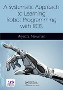
The following lines, declaring a transmission and actuator, are also required to interface with ROS controllers:
The controller plug-in library is included in the URDF with the following lines:

(The model also includes a simulated force sensor, but discussion of this is deferred for now.)
The ROS control plug-in includes options for both position and velocity controllers. The specific controller to be used is established by launching appropriate nodes.
11.2 Example position controller
The launch file prismatic1dofrobotwjntposctl.launch contains:

This launch file loads control parameters from file onedofposctlparams.yaml, converts the model xacro file into a URDF file and loads it on the parameter server, spawns the robot model into Gazebo for simulation, and loads the controller joint1positioncontroller. The controller parameters must be consistent with the chosen type (position controller). Further, the joint name associated with the controller (joint1) must be part of the controller name loaded.
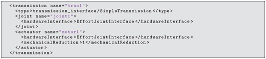
The YAML file with control parameters, onedofposctlparams.yaml, is listed below:
The control parameter file must reference the name of the robot (oneDOFrobot), and for each joint (only joint1 in this case), the position-control gains must be listed. In the example, the proportional gain is 400 N/m, and all other gains are suppressed to zero. Damping is provided implicit to the joint definition (which contains the specification: ). In fact, the derivative gain in the default position controller is quite noisy, presumably due to use of backwards-difference velocity estimates. Implicit joint damping in the robot model is better behaved than derivative feedback.
Choosing good control gains can be challenging, but ROS offers tools that can help. A detailed tutorial can be found at http://www.w3.org/1999/xlink. In choosing gains, one must keep in mind that the physics engine runs with a default time step of 1 ms, and thus control bandwidths must be designed to accommodate this limitation. For 1 kHz update rate, controllers should be limited (roughly) to less than 100 Hz bandwidth. In practice, numerical artifacts appear well below this frequency. For the one-DOF example, the mass of link2 was set to 1 kg, and the proportional gain was set to 400. The undamped natural frequency of the system is thus rad/sec, or about 3 Hz.
The system response to sinusoidal command inputs can be observed using rqtplot, and control gains can be adjusted interactively using rqtgui. Sinusoidal command inputs can also be specified using rqtgui. In the examplecontrollers package, an alternative excitation node called onedofsinecommander, prompts for frequency and amplitude and publishes sinusoidal commands to the joint1 command topic. The system can be tested as follows. First, start Gazebo with:

Then spawn the robot and its controller with the associated control gains using:

Start rqtgui and rqtplot:

Choose topics to plot in rqtplot to be oneDOFrobot/joint1positioncontroller/command/data, oneDOFrobot/jointstates/position[0], and oneDOFrobot/jointstates/effort[0].
Using rqtgui is somewhat involved, as it presents many options. One can add a MessagePublisher and select the topic oneDOFrobot/joint1positioncontroller/ command. Expanding this topic, the sole item is data. One can edit the expression value on this row to define the command to be published. This can be as simple as a constant value, or it can be an expression to be evaluated dynamically (typically, a sinusoidal function).
In a separate panel of rqtgui, one can perform dynamic reconfigure to vary control gains interactively. Expanding the joint1 control topic down to the level of PID exposes sliders for the control gains. These will be initialized to the values in the control-parameter YAML file. They can be adjusted while the robot is running, so one can immediately observe their effects in rqtplot.
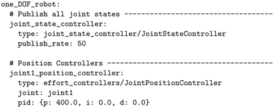
Figure 11.1 shows a snapshot of this process. The Gazebo window shows the robot; the rqtgui window shows the selection of joint command publisher and PID values; and the rqtplot window shows the transient response of position command, actual position, and control effort due to a step in command from m to m. The control effort in Fig 11.1 is large, squeezing the displacement response to a small range. Figure 11.2 shows a zoom of this transient to reveal the step command (in red) and the position response (in cyan). The response shows several overshoots and convergence over roughly half a second. Alternatively, the published stimulus can be a sinusoid, as shown in Fig 11.3. For this case, the published command is the function 0.1*sin(i/5)-0.5, which is a sinusoid of amplitude 0.1 m, offset by m (which is the middle of the joint’s range of motion). The frequency follows from the publication rate, which is set to 100 Hz. The value of “i” increments at this rate, and thus the frequency of this sinusoid is 20 rad/sec. Since our undamped natural frequency is 20 rad/sec, we expect to see poor tracking at this frequency. As expected, the position response lags the command by a phase of 90 degrees at this frequency of excitation. The PID sliders can be varied to test alternative gains and their influence on response to step inputs or sinusoids.
Figure 11.1 Servo tuning process for one-DOF robot

Figure 11.2 Servo tuning process for one-DOF robot: zoom on position response
A limitation of the position controller is that the derivative gain does not accept velocity feed-forward commands. Consequently, dynamic tracking performance is limited. An alternative is to use a ROS velocity controller instead of a position controller, and to perform position feedback via an external node (a successive loop closure technique).
11.3 Example velocity controller
An alternative launch file that references the same robot model is prismatic1dofrobotwjntvelctl.launch, which contains:
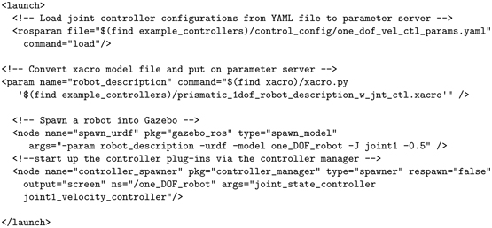
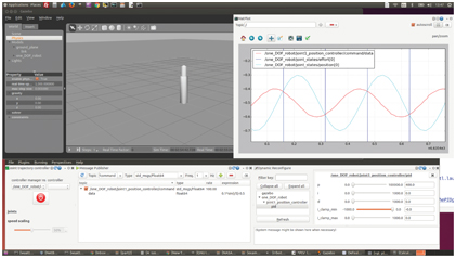
Figure 11.3 Servo tuning process for one-DOF robot: 20 rad/sec sinusoidal command
As with the position controlled launch, this launch file loads control parameters from a file (onedofvelctlparams.yaml), converts the model xacro file into a URDF file and loads it on the parameter server, spawns the robot model into Gazebo for simulation, and loads a controller (joint1velocitycontroller instead of joint1positioncontroller). Again, the joint name associated with the controller (joint1) must be part of the controller name loaded (joint1velocitycontroller). In this launch file, an additional option used in spawning the model is -J joint1 -0.5. This initializes the robot’s joint1 position to the middle of its range of motion.
The YAML file with control parameters, onedofvelctlparams.yaml, is listed below:

This file references the robot name (oneDOFrobot) and the joint name(s) (joint1). The same process is used to analyze the velocity controller. First, start Gazebo:

The robot is then spawned using the alternative launch file and gains:

The rqtgui and rqtplot tools are started:

Within rqtgui, the joint1velocitycontroller is adjusted to change the velocity gain “P”. The commanded and actual joint velocities are plotted, as shown in Fig 11.4, and the responses to commands can be observed as the gain is varied.
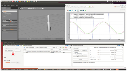
Figure 11.4 Velocity controller tuning process for one-DOF robot
The commanded velocity for the example shown in Fig 11.4 came from a separate node:

This node prompts the user for an amplitude and frequency. The responses for the case of Fig 11.4 were 0.1 m and 3 Hz.
Analysis of the velocity controller is somewhat more difficult, since link2 can drift from its center to hit its displacement limits, which introduces distortions when attempting to tune gains. To address this, two adjustments were made. First, gravity was set to zero in Gazebo, so link2 would not collapse to its lowest level. Second, the robot was started with joint1 in the the middle of its range of motion. Although it may drift from this average position over time, this placement allows some time to obtain performance data before interacting with joint limits. An outer loop that considers position can correct for the drift of velocity control. An example is presented next in the context of force feedback.
11.4 Example force controller
A third style of control incorporates consideration of interaction forces to achieve programmable compliance. The one-DOF prismatic robot model includes the following lines to emulate a force–torque sensor:
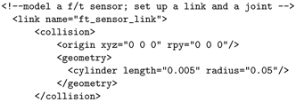
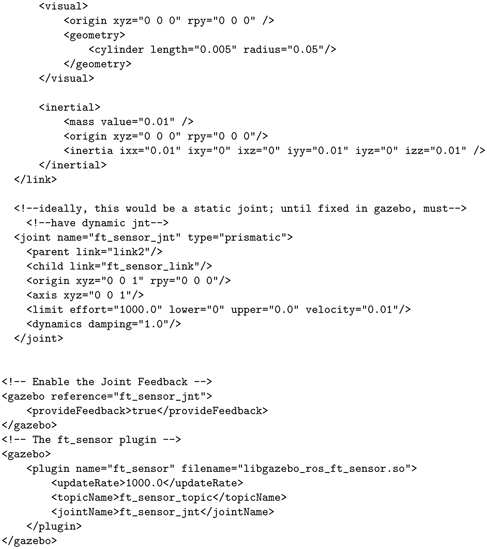
An additional link, ftsensorlink, is defined with visual, collision and inertial properties. This link is connected to parent link2 via a joint defined as ftsensorjnt. Ideally, this would be a static joint, but Gazebo (at present) requires that the joint be movable. It is thus defined as a prismatic joint, but with equal lower and upper joint limits.
A Gazebo tag brings in the plug-in libgazeborosftsensor.so, which is associated with the ftsensorjnt and configured to publish its data to topic ftsensortopic.
When this model is spawned, the topic ftsensortopic shows up, and:

shows that this topic carries messages of type geometrymsgs/WrenchStamped.
If we start the position-controlled one-DOF robot:

then command a position of for joint1 (i.e. nearly fully extended), we can observe transients as we drop a weight on the robot, using:

This introduces a large cylinder model into Gazebo at an initial height of 4 m. The cylinder has a mass of 10 kg and falls towards the ground plane under the influence of gravity (which was reduced to for this example). Figure 11.5 shows the response. Due to the additional mass supported by the robot, the resonant frequency and the damping are reduced, resulting in many oscillations before settling down. The force sensor sees a spike of impact when the weight makes contact. As link2 rebounds, the weight is tossed back in the air, and it subsequently makes three more impacts (and loses contact three more times) before the robot and weight maintain steady contact. From this point on, the robot and payload dynamics is linear, producing a sinusoidal motion due to the robot’s position controller acting like a spring.
The actuator effort has the opposite sign as the force-sensor z value, and the actuator effort magnitude is 5 N greater than that of the sensor value. This is because the actuator is supporting the weight of the payload (10 kg) plus the weight of link2 (1 kg), whereas the force sensor is influenced only by the weight of the payload.

Figure 11.5 Force sensor and actuator effort due to dropping 10 kg weight on one-DOF robot
An anomaly of this example is that the joint effort and force sensor equilibrate to the wrong values. In steady state, the actuator effort should balance the weight of link2 plus payload, which should be the weight of the 1 kg link2 plus 10 kg cylinder. Instead, the system equilibrates to the equivalent of supporting slightly more than 7 kg. This error may be related to the physics engine’s difficulty handling sustained contact.
The behavior of the position controller responding to the dropped weight is a mass-spring-damper system. However, the response is somewhat unrealistic, since the model has zero Coulomb friction and the transmission is perfectly back-driveable. A similar response can be obtained from more realistic robots by commanding velocities that would correspond to an ideal mass-spring-damper system. An implementation is given within the examplecontrollers package as naccontroller.cpp. This node subscribes to the joint state and to the force sensor topic. Within a tight loop it deduces the acceleration that would occur if the system were an ideal mass-spring-damper being acted on by forces exerted at the force sensor location. The values of the virtual mass, stiffness and damping to be emulated are contained within the variables Mvirt, Kvirt and Bvirt, respectively. The key lines within the main loop of naccontroller.cpp are:

In the above, fvirt is a virtual force comprised of two terms. The first term is the force exerted by a virtual spring of stiffness Kvirt stretched between an attractor position, xattractor, and the actual position of link2, glink2pos, as reported by the joint state publisher. The second term is due to a virtual damper of damping Bvirt acting between a reference at zero velocity and link2 moving at velocity glink2vel, also as reported by the joint-state publisher.
In addition to the virtual forces, a physical force is exerted at the robot’s endpoint, which is sensed by the force sensor. The value of sensed force in the z direction, gforcez, is obtained by subscribing to the force sensor topic. The sum of the sensed physical force and the virtual forces is the net force, fnet. A virtual mass, Mvirt, acted on by this net force would have an acceleration, accideal, of fnet/Mvirt. Correspondingly, the velocity of this mass, videal, is the time integral of the ideal acceleration. This model-based velocity is then sent as a command to a stiff velocity controller. Preferably, the value of Mvirt should be close to the actual mass of link2 (thus making this controller a natural admittance controller).
To run this controller, again start Gazebo:

Then spawn the robot using velocity control:

Then start the NAC node:

The example NAC controller was assigned values of Mvirt = 1.0 kg, Kvirt = 1000 N/m and Bvirt = 50 N/(m/sec). With this controller running and gravity set to , the 10 kg weight was dropped on the robot, resulting in the transient shown in Figure 11.6. By tuning the values of Kvirt and Bvirt, the transient behavior can be adjusted to a desirable response.
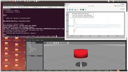
Figure 11.6 NAC controller response to dropping 10 kg weight on one-DOF robot
Although the controllers here have been illustrated only in one degree of freedom, the approach generalizes to complex arms. Figure 11.7 shows a seven-DOF arm holding a weight using natural admittance control. Source code for this example is in package arm7dofnaccontroller. Conceptually, the approach is the same as the one-DOF controller. Sensed forces and virtual forces are combined (as vectors rather than scalars), and robot inertia (a matrix, rather than a constant) is considered to compute accelerations (in joint space) expected to result from the effort interactions. The joint accelerations are integrated to compute equivalent joint velocities, and these velocities are commanded to joint velocity servos of the robot.
As a result, the seven-DOF arm behaves like a mass-spring-damper system. It catches a dropped weight gracefully, without excessive impact forces or oscillations.
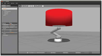
Figure 11.7 Seven-DOF arm catching and holding weight using NAC
11.5 Trajectory messages for robot arms
In ROS, the conventional means to execute a joint space motion plan is to populate a trajectory message and send it to a trajectory execution action server.
As described within a URDF file, a robot model consists of a collection (a tree) of robot links, connected pair-wise via joints. Each joint allows a single degree of freedom of motion: a rotation or a translation. Either type of motion may be referred to generically as a displacement. Displacement commands are input to low-level servo controllers, which exert torques or forces (generically referred to as efforts) to attempt to achieve a desired state. The desired state is comprised of desired displacements, possibly augmented by desired velocities, possibly further augmented by desired accelerations. The controller compares the desired state to the actual (measured) state to derive a control effort, to be imposed by the respective actuator.
If the desired state is too far from the actual state, the controller will try to exert unreasonable efforts, resulting in effort saturation and leading to poor following of or convergence to desired states. The resulting motion can be unpredictable and dangerous.
In order for the robot to achieve a desirable motion, motion commands should be evaluated in advance to make sure they are achievable within the following constraints:
- The robot should not hit objects in its environment.
- The path in joint space should conform to the constraints of minimum and maximum range of motion of the joints.
- The joint velocities should remain within the velocity limits of the respective actuators.
- The required joint efforts should remain within the effort limits of the actuators.
The first two requirements are imposed on path planning. The path defines a sequence of poses to be realized. The second two requirements are imposed on trajectory planning, which augments a path with timing. To convert a path to a trajectory, one must augment each pose with an arrival time (time from start of motion) computed such that velocity and effort constraints are satisfied.
One condition to avoid is a step command to any joint. If a joint is commanded to move instantaneously from A to B, the motion will be physically impossible to achieve, and the resulting behavior will likely be undesirable.
A necessary (but not sufficient) requirement of a safe robot command is that the command should be updated frequently (e.g. 100 Hz or faster is typical), and the commands should form an approximation of a smooth, continuous stream for all joints.
Since this is a common requirement, ROS includes a message type for this style of command: trajectorymsgs/JointTrajectory.
Invoking:

shows that this message consists of the following fields:
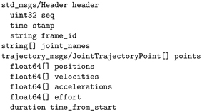
In the header, the frameid is not meaningful, since the commands are in joint space (desired state of each joint).
The vector of strings jointnames should be populated with text names assigned to the joints (consistent with naming in the URDF file). For a serial chain robot, joints are conventionally known by integers, starting from joint 1, the joint closest to ground (most proximal joint), and progressing sequentially to the most distal joint. However, robots with multiple arms and/or legs are not so easily described, and thus names are introduced.
In specifying a vector of desired joint displacements, one must associate the joint commands with the corresponding joint names. Generally, there is no requirement to specify the joint commands in any specific order or requirement to specify all joint commands on every iteration. For example, one might command a neck rotation only in one instance, then follow that by a separate command to a subset of joints of the right arm, etc. However, some packages require that all joint states be specified in every command (whether or not it is desired to move all joints). Other packages receiving trajectory messages might implicitly depend on specifying joint commands in a specific, fixed order, ignoring the jointnames field (although this is not preferred).
The bulk of the trajectory message is a vector of type trajectorymsgs/JointTrajectoryPoint. This type contains four variable-length vectors and a duration. A trajectory command can use as few as one of these fields and as many as all four. One common minimal usage is to specify only the joint displacements in the positions vector. This can be adequate, particularly for low-speed motions controlled by joint position feedback. Alternatively, the trajectory command might communicate with a velocity controller, e.g. for speed control of wheels. A more sophisticated motion plan communicating with a more sophisticated joint controller would include multiple fields (specifying both positions and velocities is common).
To command coordinated motion of all seven joints of a seven-DOF arm, for example, one would populate (at least) the positions vector for each of N points to visit, starting from the current pose and ending at some desired pose. Preferably, these points would be relatively close in space (i.e. with relatively small changes in any one joint displacement command between sequential point specifications). Alternatively, coarser trajectories may be communicated to a trajectory interpolator, which breaks up motions between coarse subgoals into streams of fine motion commands.
It is desirable that each point include specification of joint velocities that are consistent with the specified displacements and arrival times (although it is legal to specify a trajectory without specifying joint velocities). Alternatively, generation of consistent velocity commands might be left to a lower-level trajectory interpolator node.
Each joint-space point to be visited must specify a timefromstart. These time specifications must be monotonically increasing for sequential points and should be consistent with the velocity specifications. It is the user’s responsibility to evaluate whether the specified joint displacements, joint velocities and point arrival times are all self-consistent and achievable within the robot’s limitations.
The timefromstart value, specified for each joint-space point to be visited, distinguishes a path from a trajectory. If one were to specify only the sequence of poses to be realized, the result would be a path description. By augmenting space (path) information with time, the result is a trajectory (in joint space).
While a trajectory message may be fine-grained and lengthy, it is more common (and practical) to send messages that consist of a sequence of subgoals (with adequate resolution). Fine-grained commands can be generated by interpolation via an action server. An illustrative example is provided in the package exampletrajectory.
In this package, an action message is defined: TrajAction.action. The goal field of this action message contains trajectorymsgs::JointTrajectory. This action message is used by a trajectory client to send goals to a trajectory action server.
Two illustrative nodes are the exampletrajectoryactionclient and exampletrajectoryactionserver. The client computes a desired trajectory, in this case consisting of samples of a sinusoidal motion of joint1. (This could easily be extended to N joints, but this is sufficient for testing on the minimalrobot.) The samples are deliberately taken at irregular and fairly coarse time intervals. An example output is shown in Fig 11.8. The values of position command (radians) show that the originating sinusoidal function is sampled coarsely and irregularly. This was done to illustrate the generality of the trajectory message, and show that it need not be fine grained.
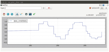
Figure 11.8 Coarse trajectory published at irregularly sampled points of sine wave
The joint command samples are packaged into a trajectory message along with associated arrival times, and this message is transmitted to the trajectory action server within the action goal.
The exampletrajectoryactionserver receives the goal message and interpolates linearly between specified points, resulting in the profile shown in Fig 11.9. The resulting profile is piece-wise linear, but sufficiently smooth; the minimalrobot can follow this command reasonably well, yielding a smooth motion.

Figure 11.9 Action-server linear interpolation of coarse trajectory
The example is run with:

which brings up the one-DOF robot and its controller. The trajectory interpolation action server is started with:

and the corresponding trajectory client is started with:

This client generates a coarse trajectory and sends it to the action server within a goal message. In turn, the action server interpolates this trajectory and sends a fast, smooth stream of commands to the robot.
For the example trajectory action server, the velocities specified by the client in the goal message are ignored. In the one-DOF robot case, the minimal joint controller does not accept velocity feed-forward commands. More generally, one could do better with a servo controller that accepts both position and velocity feed-forward commands. In this case, including consistent velocity commands sent to the servo controller would improve tracking performance. These velocity commands could be generated on the fly by the trajectory interpolator or included in a longer, fine-grained trajectory message.
The example trajectory interpolator is piece-wise linear. It would also be desirable to have a smoother interpolator, e.g. cubic splines. (See e.g. http://www.w3.org/1999/xlink for a joint trajectory action server for the Baxter robot, written in Python, which uses cubic spline interpolation.)
The intelligence of the trajectory action server is a design decision. Optimizing a trajectory with considerations of speed, precision and collision avoidance is a computationally difficult problem. Further, the optimization criteria may change from one instance to another. The trajectory specification, even if it is coarse, must still take into consideration issues of collisions and speed and effort constraints. Rather than perform this optimization twice (for construction of a viable trajectory, further smoothing and optimization of that trajectory by the action server), one could perform trajectory optimization as part of the planning process that generates a trajectory specification. This could yield a dense sampling of points in the trajectory specification, along with compatible velocities, accelerations and gravity load compensation. If this approach is taken, then linear interpolation of the dense trajectory commands should be adequate in general, although the trajectory action server should also pass along the corresponding velocity and effort values contained within these optimized trajectories.
Trying to make the trajectory action server more intelligent than mere linear interpolation is thus not warranted and may, in fact, interfere with optimization of pre-computed trajectories. Thus, this simple example may be considered adequate in general.
This discussion of trajectory messages applies directly to ROS-Industrial (see http://www.w3.org/1999/xlink). To bridge ROS to existing industrial robots, one can write the equivalent of the exampletrajectoryactionserver in the native language of the target robot (and run it on the native robot controller). This (non-ROS) program also requires custom communications to receive packets containing the equivalent of trajectory messages. A complementary ROS node would receive trajectory messages via a ROS topic or ROS goal message, translate them into the format expected by the robot’s communication program, and transmit the corresponding packets to the robot controller for interpolation and execution.
Correspondingly, the robot controller would also run a program that samples and transmits the robot’s joint state (at least the joint angles). A ROS node would receive these values in some custom format, translate them into ROS sensormsgs::JointState messages and publish these on the topic jointstates for use by other ROS nodes (including rviz). Using this approach, the ROS-Industrial consortium has retrofit ROS interfaces to a growing number of industrial robots.
11.6 Trajectory interpolation action server for a seven-DOF arm
The package arm7doftrajas contains a helpful library, arm7doftrajectorystreamer, and an action server, arm7dofactionserver extends the minimal-robot example to seven degrees of freedom. This action server responds to goal messages that contain joint-space trajectories. The incoming trajectories may be coarse, since they are interpolated at 50 Hz (a parameter defined in the header file arm7doftrajectorystreamer.h).
An example client program, arm7doftrajactionclientprompter, illustrates use of the trajectory action server. This example client first sends the robot to a hard-coded pose, then prompts the user to enter joint numbers and joint values, which it then commands to the robot via the trajectory action server. To run this example, first start Gazebo:

Next, bring up the seven-DOF robot arm with its position controllers, using:

Note that these two steps are required only for robot simulation. When interacting with a real robot with a ROS interface, the actual robot dynamics takes the place of Gazebo’s physics engine, and the real controllers take the places of the ROS controllers. Typically, the physical robot would host the roscore. The robot would expose its topics for publishing robot state and receiving joint commands.
Next, running:

brings up the trajectory action server, which provides a trajectory interface between low-level joint angle commands and higher-level trajectory plans. This node should be run during both simulation and physical operation.
An example interactive trajectory client can be started with:

This will pre-position the robot, then accept commands from the user (one joint at a time). More generally, a trajectory client would be instantiated within a higher-level application that performs trajectory planning, presumably based on sensory information.
The seven-DOF trajectory-interpolation action server here will be modified slightly to apply it to the left and right arms of a Baxter robot, which will be introduced in Chapter 14.
11.7 Wrap-Up
This chapter has presented low-level joint-control options in ROS, including position control, velocity control, and extensions to force control with respect to a force–torque sensor (available as a plug-in in Gazebo). At the joint level, smooth and coordinated motion is achieved using a joint-space interpolator that operates on trajectory messages. Higher-level controls, e.g. for Cartesian motion control, ultimately depend on lower-level control in joint space.
Building on joint-level control, we next consider how to compute desirable joint-space trajectories with consideration of desirable end-effector motion. This is the subject of forward and inverse kinematics, which is discussed next.