

Design and Analysis of Single-Factor Experiments: The Analysis of Variance

Chapter Outline
13-1 Designing Engineering Experiments
13-2 Completely Randomized Single-Factor Experiment
13-2.1 Example: Tensile Strength
13-2.3 Multiple Comparisons Following the ANOVA
13-2.4 Residual Analysis and Model Checking
13-2.5 Determining Sample Size
13-3.1 Fixed Versus Random Factors
13-3.2 ANOVA and Variance Components
13-4 Randomized Complete Block Design
Experiments are a natural part of the engineering and scientific decision-making process. Suppose, for example, that a civil engineer is investigating the effects of different curing methods on the mean compressive strength of concrete. The experiment would consist of making up several test specimens of concrete using each of the proposed curing methods and then testing the compressive strength of each specimen. The data from this experiment could be used to determine which curing method should be used to provide maximum mean compressive strength.
If there are only two curing methods of interest, this experiment could be designed and analyzed using the statistical hypothesis methods for two samples introduced in Chapter 10. That is, the experimenter has a single factor of interest—curing methods—and there are only two levels of the factor. If the experimenter is interested in determining which curing method produces the maximum compressive strength, the number of specimens to test can be determined from the operating characteristic curves in Appendix Chart VII, and the t-test can be used to decide if the two means differ.
Many single-factor experiments require that more than two levels of the factor be considered. For example, the civil engineer may want to investigate five different curing methods. In this chapter, we show how the analysis of variance (frequently abbreviated ANOVA) can be used for comparing means when there are more than two levels of a single factor. We also discuss randomization of the experimental runs and the important role this concept plays in the overall experimentation strategy. In the next chapter, we show how to design and analyze experiments with several factors.
After careful study of this chapter, you should be able to do the following:
- Design and conduct engineering experiments involving a single factor with an arbitrary number of levels
- Understand how the analysis of variance is used to analyze the data from these experiments
- Assess model adequacy with residual plots
- Use multiple comparison procedures to identify specific differences between means
- Make decisions about sample size in single-factor experiments
- Understand the difference between fixed and random factors
- Estimate variance components in an experiment involving random factors
- Understand the blocking principle and how it is used to isolate the effect of nuisance factors
- Design and conduct experiments involving the randomized complete block design
13-1 Designing Engineering Experiments
Statistically based experimental design techniques are particularly useful in the engineering world for solving many important problems: discovery of new basic phenomena that can lead to new products and commercialization of new technology including new product development, new process development, and improvement of existing products and processes. For example, consider the development of a new process. Most processes can be described in terms of several controllable variables, such as temperature, pressure, and feed rate. By using designed experiments, engineers can determine which subset of the process variables has the greatest influence on process performance. The results of such an experiment can lead to
- Improved process yield
- Reduced variability in the process and closer conformance to nominal or target requirements
- Reduced design and development time
- Reduced cost of operation
Experimental design methods are also useful in engineering design activities during which new products are developed and existing ones are improved. Some typical applications of statistically designed experiments in engineering design include
- Evaluation and comparison of basic design configurations
- Evaluation of different materials
- Selection of design parameters so that the product will work well under a wide variety of field conditions (or so that the design will be robust)
- Determination of key product design parameters that affect product performance
The use of experimental design in the engineering design process can result in products that are easier to manufacture, products that have better field performance and reliability than their competitors, and products that can be designed, developed, and produced in less time.
Designed experiments are usually employed sequentially. That is, the first experiment with a complex system (perhaps a manufacturing process) that has many controllable variables is often a screening experiment designed to determine those variables are most important. Subsequent experiments are used to refine this information and determine which adjustments to these critical variables are required to improve the process. Finally, the objective of the experimenter is optimization, that is, to determine those levels of the critical variables that result in the best process performance.
Every experiment involves a sequence of activities:
- Conjecture—the original hypothesis that motivates the experiment.
- Experiment—the test performed to investigate the conjecture.
- Analysis—the statistical analysis of the data from the experiment.
- Conclusion—what has been learned about the original conjecture from the experiment. Often the experiment will lead to a revised conjecture, a new experiment, and so forth.
The statistical methods introduced in this chapter and Chapter 14 are essential to good experimentation. All experiments are designed experiments; unfortunately, some of them are poorly designed, and as a result, valuable resources are used ineffectively. Statistically designed experiments permit efficiency and economy in the experimental process, and the use of statistical methods in examining the data results in scientific objectivity when drawing conclusions.
13-2 Completely Randomized Single-Factor Experiment
13-2.1 EXAMPLE: TENSILE STRENGTH
A manufacturer of paper used for making grocery bags is interested in improving the product's tensile strength. Product engineering believes that tensile strength is a function of the hardwood concentration in the pulp and that the range of hardwood concentrations of practical interest is between 5 and 20%. A team of engineers responsible for the study decides to investigate four levels of hardwood concentration: 5%, 10%, 15%, and 20%. They decide to make up six test specimens at each concentration level by using a pilot plant. All 24 specimens are tested on a laboratory tensile tester in random order. The data from this experiment are shown in Table 13-1.
This is an example of a completely randomized single-factor experiment with four levels of the factor. The levels of the factor are sometimes called treatments, and each treatment has six observations or replicates. The role of randomization in this experiment is extremely important. By randomizing the order of the 24 runs, the effect of any nuisance variable that may influence the observed tensile strength is approximately balanced out. For example, suppose that there is a warm-up effect on the tensile testing machine; that is, the longer the machine is on, the greater the observed tensile strength. If all 24 runs are made in order of increasing hardwood concentration (that is, all six 5% concentration specimens are tested first, followed by all six 10% concentration specimens, etc.), any observed differences in tensile strength could also be due to the warm-up effect. The role of randomization to identify causality was discussed in Section 10-1.
It is important to graphically analyze the data from a designed experiment. Figure 13-1(a) presents box plots of tensile strength at the four hardwood concentration levels. This figure indicates that changing the hardwood concentration has an effect on tensile strength; specifically, higher hardwood concentrations produce higher observed tensile strength. Furthermore, the distribution of tensile strength at a particular hardwood level is reasonably symmetric, and the variability in tensile strength does not change dramatically as the hardwood concentration changes.
![]() TABLE • 13-1 Tensile Strength of Paper (psi)
TABLE • 13-1 Tensile Strength of Paper (psi)

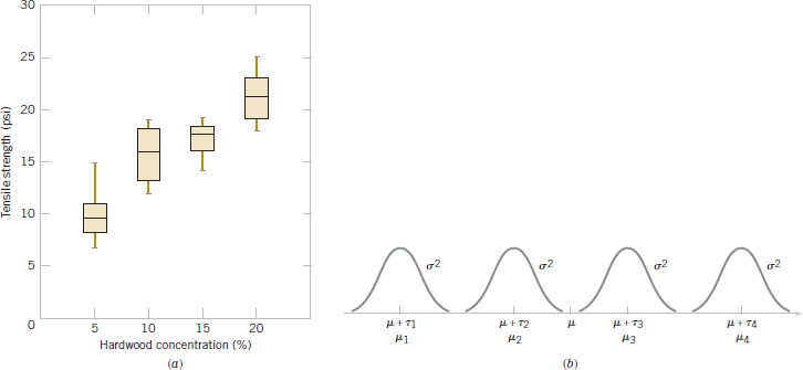
FIGURE 13-1 (a) Box plots of hardwood concentration data. (b) Display of the model in Equation 13-1 for the completely randomized single-factor experiment.
Graphical interpretation of the data is always useful. Box plots show the variability of the observations within a treatment (factor level) and the variability between treatments. We now discuss how the data from a single-factor randomized experiment can be analyzed statistically.
13-2.2 ANALYSIS OF VARIANCE
Suppose that we have a different levels of a single factor that we wish to compare. Sometimes, each factor level is called a treatment, a very general term that can be traced to the early applications of experimental design methodology in the agricultural sciences. The response for each of the a treatments is a random variable. The observed data would appear as shown in Table 13-2. An entry in Table 13-2, say yij, represents the jth observation taken under treatment i. We initially consider the case that has an equal number of observations, n, on each treatment.
We may describe the observations in Table 13-2 by the linear statistical model
![]()
where yij is a random variable denoting the (ij)th observation, μ is a parameter common to all treatments called the overall mean, τi is a parameter associated with the ith treatment called the ith treatment effect, and ![]() ij is a random error component. Notice that the model could have been written as
ij is a random error component. Notice that the model could have been written as
![]()
where μi = μ + τi is the mean of the ith treatment. In this form of the model, we see that each treatment defines a population that has mean μi consisting of the overall mean μ plus an effect τi that is due to that particular treatment. We assume that the errors ![]() ij are normally and independently distributed with mean zero and variance σ2. Therefore, each treatment can be thought of as a normal population with mean μi and variance σ2. See Fig. 13-1(b).
ij are normally and independently distributed with mean zero and variance σ2. Therefore, each treatment can be thought of as a normal population with mean μi and variance σ2. See Fig. 13-1(b).
![]() TABLE • 13-2 Typical Data for a Single-Factor Experiment
TABLE • 13-2 Typical Data for a Single-Factor Experiment

Equation 13-1 is the underlying model for a single-factor experiment. Furthermore, because we require that the observations are taken in random order and that the environment (often called the experimental units) in which the treatments are used is as uniform as possible, this experimental design is called a completely randomized design (CRD).
The a factor levels in the experiment could have been chosen in two different ways. First, the experimenter could have specifically chosen the a treatments. In this situation, we wish to test hypotheses about the treatment means, and conclusions cannot be extended to similar treatments that were not considered. In addition, we may wish to estimate the treatment effects. This is called the fixed-effects model. Alternatively, the a treatments could be a random sample from a larger population of treatments. In this situation, we would like to be able to extend the conclusions (which are based on the sample of treatments) to all treatments in the population whether or not they were explicitly considered in the experiment. Here the treatment effects τi are random variables, and knowledge about the particular ones investigated is relatively unimportant. Instead, we test hypotheses about the variability of the τi and try to estimate this variability. This is called the random-effects, or components of variance model.
In this section, we develop the analysis of variance for the fixed-effects model. The analysis of variance is not new to us; it was used previously in the presentation of regression analysis. However, in this section, we show how it can be used to test for equality of treatment effects. In the fixed-effects model, the treatment effects τi are usually defined as deviations from the overall mean μ, so that
![]()
Let yi. represent the total of the observations under the ith treatment and ![]() i. represent the average of the observations under the ith treatment. Similarly, let y.. represent the grand total of all observations and
i. represent the average of the observations under the ith treatment. Similarly, let y.. represent the grand total of all observations and ![]() .. represent the grand mean of all observations. Expressed mathematically,
.. represent the grand mean of all observations. Expressed mathematically,

where N = an is the total number of observations. Thus, the “dot” subscript notation implies summation over the subscript that it replaces.
We are interested in testing the equality of the a treatment means μ1, μ2,..., μa. Using Equation 13-2, we find that this is equivalent to testing the hypotheses
![]()
Thus, if the null hypothesis is true, each observation consists of the overall mean μ plus a realization of the random error component ![]() ij. This is equivalent to saying that all N observations are taken from a normal distribution with mean μ and variance σ2. Therefore, if the null hypothesis is true, changing the levels of the factor has no effect on the mean response.
ij. This is equivalent to saying that all N observations are taken from a normal distribution with mean μ and variance σ2. Therefore, if the null hypothesis is true, changing the levels of the factor has no effect on the mean response.
The ANOVA partitions the total variability in the sample data into two component parts. Then, the test of the hypothesis in Equation 13-4 is based on a comparison of two independent estimates of the population variance. The total variability in the data is described by the total sum of squares
![]()
The partition of the total sum of squares is given in the following definition.
ANOVA Sum of Squares Identity: Single Factor Experiment
The sum of squares identity is
![]()
or symbolically
![]()
The identity in Equation 13-5 shows that the total variability in the data, measured by the total corrected sum of squares SST, can be partitioned into a sum of squares of differences between treatment means and the grand mean called the treatment sum of squares, and denoted SSTreatments and a sum of squares of differences of observations within a treatment from the treatment mean called the error sum of squares, and denoted SSE. Differences between observed treatment means and the grand mean measure the differences between treatments, and differences of observations within a treatment from the treatment mean can be due only to random error.
We can gain considerable insight into how the analysis of variance works by examining the expected values of SSTreatments and SSE. This will lead us to an appropriate statistic for testing the hypothesis of no differences among treatment means (or all τi = 0).
Expected Values of Sums of Squares: Single Factor Experiment
The expected value of the treatment sum of squares is
![]()
and the expected value of the error sum of squares is
![]()
There is also a partition of the number of degrees of freedom that corresponds to the sum of squares identity in Equation 13-5. That is, there are an = N observations; thus, SST has an − 1 degrees of freedom. There are a levels of the factor, so SSTreaments has a − 1 degrees of freedom. Finally, within any treatment, there are n replicates providing n − 1 degrees of freedom with which to estimate the experimental error. Because there are a treatments, we have a(n − 1) degrees of freedom for error. Therefore, the degrees of freedom partition is
![]()
The ratio
![]()
is called the mean square for treatments. Now if the null hypothesis H0: τ1 = τ2 = ··· = τa = 0 is true, MSTreatments is an unbiased estimator of σ2 because ![]() . However, if H1 is true, MSTreatments estimates σ2 plus a positive term that incorporates variation due to the systematic difference in treatment means.
. However, if H1 is true, MSTreatments estimates σ2 plus a positive term that incorporates variation due to the systematic difference in treatment means.
Note that the mean square for error
![]()
is an unbiased estimator of σ2 regardless of whether or not H0 is true. We can also show that MSTreatments and MSE are independent. Consequently, we can show that if the null hypothesis H0 is true, the ratio
ANOVA F-Test

has an F-distribution with a − 1 and a(n − 1) degrees of freedom. Furthermore, from the expected mean squares, we know that MSE is an unbiased estimator of σ2. Also, under the null hypothesis, MSTreatments is an unbiased estimator of σ2. However, if the null hypothesis is false, the expected value of MSTreatments is greater than σ2. Therefore, under the alternative hypothesis, the expected value of the numerator of the test statistic (Equation 13-7) is greater than the expected value of the denominator. Consequently, we should reject H0 if the statistic is large. This implies an upper-tailed, one-tailed critical region. Therefore, we would reject H0 if f0 > fα,a−1,a(n−1) where f0 is the computed value of F0 from Equation 13-7.
Efficient computational formulas for the sums of squares may be obtained by expanding and simplifying the definitions of SSTreatments and SST. This yields the following results.
Computing Formulas for ANOVA: Single Factor with Equal Sample Sizes
The sums of squares computing formulas for the ANOVA with equal sample sizes in each treatment are
![]()
and
![]()
The error sum of squares is obtained by subtraction as
![]()
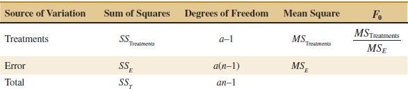
The computations for this test procedure are usually summarized in tabular form as shown in Table 13-3. This is called an analysis of variance (or ANOVA) table.
![]() TABLE • 13-3 Analysis of Variance for a Single-Factor Experiment, Fixed-Effects Model
TABLE • 13-3 Analysis of Variance for a Single-Factor Experiment, Fixed-Effects Model
Example 13-1 Tensile Strength ANOVA Consider the paper tensile strength experiment described in Section 13-2.1. This experiment is a completely randomized design. We can use the analysis of variance to test the hypothesis that different hardwood concentrations do not affect the mean tensile strength of the paper. The hypotheses are
We use α = 0.01. The sums of squares for the analysis of variance are computed from Equations 13-8, 13-9, and 13-10 as follows:
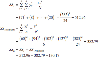
The ANOVA is summarized in Table 13-4. Because f0.01,3,20 = 4.94, we reject H0 and conclude that hardwood concentration in the pulp significantly affects the mean strength of the paper. We can also find a P-value for this test statistic as follows:
![]() TABLE • 13-4 ANOVA for the Tensile Strength Data
TABLE • 13-4 ANOVA for the Tensile Strength Data

![]()
Computer software is used here to obtain the probability. Because P ![]() 3.59 × 10⁻⁶ is considerably smaller than α = 0.01, we have strong evidence to conclude that H0 is not true.
3.59 × 10⁻⁶ is considerably smaller than α = 0.01, we have strong evidence to conclude that H0 is not true.
Practical Interpretation: There is strong evidence to conclude that hardwood concentration has an effect on tensile strength. However, the ANOVA does not tell as which levels of hardwood concentration result in different tensile strength means. We see how to answer this question in Section 13-2.3.
Computer Output
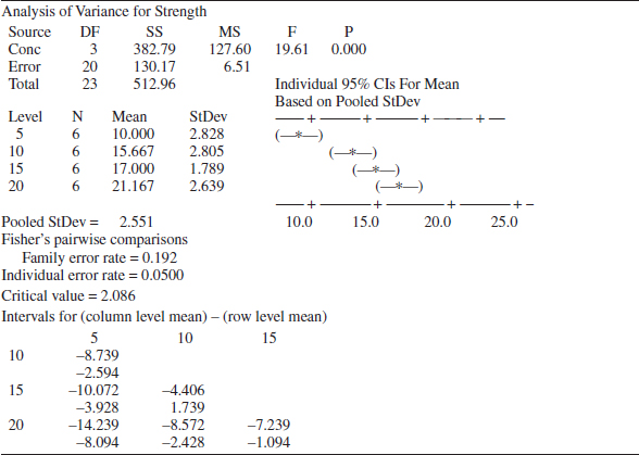
Many software packages have the capability to analyze data from designed experiments using the analysis of variance. See Table 13-5 for computer output for the paper tensile strength experiment in Example 13-1. The results agree closely with the manual calculations reported previously in Table 13-4.
The computer output also presents 95% confidece intervals (CIs) on each individual treatment mean. The mean of the ith treatment is defined as
![]()
A point estimator of μi is ![]() i =
i = ![]() i.. Now if we assume that the errors are normally distributed, each treatment average is normally distributed with mean μi and variance σ2/n. Thus, if σ2 were known, we could use the normal distribution to construct a CI. Using MSE as an estimator of σ2 (the square root of MSE is the “Pooled StDev” referred to in the computer output), we would base the CI on the t distribution, because
i.. Now if we assume that the errors are normally distributed, each treatment average is normally distributed with mean μi and variance σ2/n. Thus, if σ2 were known, we could use the normal distribution to construct a CI. Using MSE as an estimator of σ2 (the square root of MSE is the “Pooled StDev” referred to in the computer output), we would base the CI on the t distribution, because
![]()
has a t distribution with a(n − 1) degrees of freedom. This leads to the following definition of the confidence interval.
Confidence Interval on a Treatment Mean
A 100(1 − α)% confidence interval on the mean of the ith treatment μi is
![]()
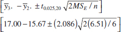
Equation 13-11 is used to calculate the 95% CIs shown graphically in the computer output of Table 13-5. For example, at 20% hardwood, the point estimate of the mean is ![]() 4. = 21.167, MSE = 6.51, and t0.025,20 = 2.086, so the 95% CI is
4. = 21.167, MSE = 6.51, and t0.025,20 = 2.086, so the 95% CI is
![]()
or
![]()
It can also be interesting to find confidence intervals on the difference in two treatment means, say, μi − μj. The point estimator of μi − μj is ![]() i. −
i. − ![]() j., and the variance of this estimator is
j., and the variance of this estimator is
![]()
![]() TABLE • 13-5 Computer Output for the Completely Randomized Design in Example 13-1
TABLE • 13-5 Computer Output for the Completely Randomized Design in Example 13-1
Now if we use MSE to estimate σ2,
![]()
has a t distribution with a(n − 1) degrees of freedom. Therefore, a CI on μi − μj may be based on the t distribution.
Confidence Interval on a Difference in Treatment Means
A 100(1 − α) percent confidence interval on the difference in two treatment means μi − μj is
![]()
A 95% CI on the difference in means μ3 − μ2 is computed from Equation 13-12 as follows:
or
![]()
Because the CI includes zero, we would conclude that there is no difference in mean tensile strength at these two particular hardwood levels.
The bottom portion of the computer output in Table 13-5 provides additional information concerning which specific means are different. We discuss this in more detail in Section 13-2.3.
Unbalanced Experiment
In some single-factor experiments, the number of observations taken under each treatment may be different. We then say that the design is unbalanced. In this situation, slight modifications must be made in the sums of squares formulas. Let ni observations be taken under treatment i(i = 1, 2,..., a), and let the total number of observations N = ![]() . The computational formulas for SST and SSTreatments are as shown in the following definition.
. The computational formulas for SST and SSTreatments are as shown in the following definition.
Computing Formulas for ANOVA: Single Factor with Unequal Sample Sizes
The sums of squares computing formulas for the ANOVA with unequal sample sizes ni in each treatment are

and
![]()
Choosing a balanced design has two important advantages. First, the ANOVA is relatively insensitive to small departures from the assumption of equality of variances if the sample sizes are equal. This is not the case for unequal sample sizes. Second, the power of the test is maximized if the samples are of equal size.
13-2.3 MULTIPLE COMPARISONS FOLLOWING THE ANOVA
When the null hypothesis H0: τ1 = τ2 = ··· = τa = 0 is rejected in the ANOVA, we know that some of the treatment or factor-level means are different. However, the ANOVA does not identify which means are different. Methods for investigating this issue are called multiple comparisons methods. Many of these procedures are available. Here we describe a very simple one, Fisher's least significant difference (LSD) method and a graphical method. Montgomery (2012) presents these and other methods and provides a comparative discussion.
The Fisher LSD method compares all pairs of means with the null hypotheses H0: μi = μj (for all i ≠ j) using the t-statistic

Assuming a two-sided alternative hypothesis, the pair of means μi and μj would be declared significantly different if
![]()
where LSD, the least significant difference, is
Least Significant Difference for Multiple Comparisons

If the sample sizes are different in each treatment, the LSD is defined as

Example 13-2 We apply the Fisher LSD method to the hardwood concentration experiment. There are a = 4 means, n = 6, MSE = 6.51, and t0.025,20 = 2.086. The treatment means are
![]()
The value of LSD is LSD = t0.025,20![]() = 2.086
= 2.086![]() = 3.07. Therefore, any pair of treatment averages that differs by more than 3.07 implies that the corresponding pair of treatment means are different.
= 3.07. Therefore, any pair of treatment averages that differs by more than 3.07 implies that the corresponding pair of treatment means are different.
The comparisons among the observed treatment averages are as follows:
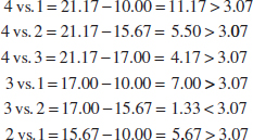

FIGURE 13-2 Results of Fisher's LSD method in Example 13-2.
Conclusions: From this analysis, we see that there are significant differences between all pairs of means except 2 and 3. This implies that 10% and 15% hardwood concentration produce approximately the same tensile strength and that all other concentration levels tested produce different tensile strengths. It is often helpful to draw a graph of the treatment means, such as in Fig. 13-2 with the means that are not different underlined. This graph clearly reveals the results of the experiment and shows that 20% hardwood produces the maximum tensile strength.
The computer output in Table 13-5 shows the Fisher LSD method under the heading “Fisher's pairwise comparisons.” The critical value reported is actually the value of t0.025,20 = 2.086. The computer output presents Fisher's LSD method by computing confidence intervals on all pairs of treatment means using Equation 13-12. The lower and upper 95% confidence limits are at the bottom of the table. Notice that the only pair of means for which the confidence interval includes zero is for μ10 and μ15. This implies that μ10 and μ15 are not significantly different, the same result found in Example 13-2.
Table 13-5 also provides a “family error rate,” equal to 0.192 in this example. When all possible pairs of means are tested, the probability of at least one type I error can be much higher than for a single test. We can interpret the family error rate as follows. The probability is 1 − 0.192 = 0.808 that there are no type I errors in the six comparisons. The family error rate in Table 13-5 is based on the distribution of the range of the sample means. See Montgomery (2012) for details. Alternatively, computer software often allows specification of a family error rate and then calculates an individual error rate for each comparison.
Graphical Comparison of Means
It is easy to compare treatment means graphically following the analysis of variance. Suppose that the factor has a levels and that ![]() 1.,
1., ![]() 2., ...,
2., ..., ![]() a. are the observed averages for these factor levels. Each treatment average has standard deviation σ/
a. are the observed averages for these factor levels. Each treatment average has standard deviation σ/![]() , where σ is the standard deviation of an individual observation. If all treatment means are equal, the observed means
, where σ is the standard deviation of an individual observation. If all treatment means are equal, the observed means ![]() i. would behave as if they were a set of observations drawn at random from a normal distribution with mean μ and standard deviation σ/
i. would behave as if they were a set of observations drawn at random from a normal distribution with mean μ and standard deviation σ/![]() .
.
Visualize this normal distribution capable of being slid along an axis below which the treatment means ![]() 1.,
1., ![]() 2., ...,
2., ..., ![]() a. are plotted. If all treatment means are equal, there should be some position for this distribution that makes it obvious that the
a. are plotted. If all treatment means are equal, there should be some position for this distribution that makes it obvious that the ![]() i. values were drawn from the same distribution. If this is not the case, the
i. values were drawn from the same distribution. If this is not the case, the ![]() i. values that do not appear to have been drawn from this distribution are associated with treatments that produce different mean responses.
i. values that do not appear to have been drawn from this distribution are associated with treatments that produce different mean responses.
The only flaw in this logic is that σ is unknown. However, we can use ![]() from the analysis of variance to estimate σ. This implies that a t distribution should be used instead of a normal distribution in making the plot, but because the t looks so much like the normal, sketching a normal curve that is approximately 6
from the analysis of variance to estimate σ. This implies that a t distribution should be used instead of a normal distribution in making the plot, but because the t looks so much like the normal, sketching a normal curve that is approximately 6![]() units wide will usually work very well.
units wide will usually work very well.
Figure 13-3 shows this arrangement for the hardwood concentration experiment in Example 13-1. The standard deviation of this normal distribution is
![]()
If we visualize sliding this distribution along the horizontal axis, we note that there is no location for the distribution that would suggest that all four observations (the plotted means) are typical, randomly selected values from that distribution. This, of course, should be expected because the analysis of variance has indicated that the means differ, and the display in Fig. 13-3 is just a graphical representation of the analysis of variance results. The figure does indicate that treatment 4 (20% hardwood) produces paper with higher mean tensile strength than do the other treatments, and treatment 1 (5% hardwood) results in lower mean tensile strength than do the other treatments. The means of treatments 2 and 3 (10% and 15% hardwood, respectively) do not differ.
This simple procedure is a rough but very effective multiple comparison technique. It works well in many situations.
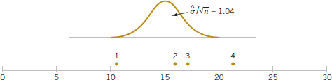
FIGURE 13-3 Tensile strength averages from the hardwood concentration experiment in relation to a normal distribution with standard deviation ![]() = 1.04.
= 1.04.
13-2.4 RESIDUAL ANALYSIS AND MODEL CHECKING
The analysis of variance assumes that the observations are normally and independently distributed with the same variance for each treatment or factor level. These assumptions should be checked by examining the residuals. A residual is the difference between an observation yij and its estimated (or fitted) value from the statistical model being studied, denoted as ![]() ij. For the completely randomized design
ij. For the completely randomized design ![]() ij =
ij = ![]() i. and each residual is eij = yij −
i. and each residual is eij = yij − ![]() i. This is the difference between an observation and the corresponding observed treatment mean. The residuals for the paper tensile strength experiment are shown in Table 13-6. Using
i. This is the difference between an observation and the corresponding observed treatment mean. The residuals for the paper tensile strength experiment are shown in Table 13-6. Using ![]() i. to calculate each residual essentially removes the effect of hardwood concentration from the data; consequently, the residuals contain information about unexplained variability.
i. to calculate each residual essentially removes the effect of hardwood concentration from the data; consequently, the residuals contain information about unexplained variability.
The normality assumption can be checked by constructing a normal probability plot of the residuals. To check the assumption of equal variances at each factor level, plot the residuals against the factor levels and compare the spread in the residuals. It is also useful to plot the residuals against ![]() i. (sometimes called the fitted value); the variability in the residuals should not depend in any way on the value of
i. (sometimes called the fitted value); the variability in the residuals should not depend in any way on the value of ![]() i. Most statistical software packages can construct these plots on request. A pattern that appears in these plots usually suggests the need for a transformation, that is, analyzing the data in a different metric. For example, if the variability in the residuals increases with
i. Most statistical software packages can construct these plots on request. A pattern that appears in these plots usually suggests the need for a transformation, that is, analyzing the data in a different metric. For example, if the variability in the residuals increases with ![]() i., a transformation such as log y or
i., a transformation such as log y or ![]() should be considered. In some problems, the dependency of residual scatter on the observed mean
should be considered. In some problems, the dependency of residual scatter on the observed mean ![]() i. is very important information. It may be desirable to select the factor level that results in maximum response; however, this level may also cause more variation in response from run to run.
i. is very important information. It may be desirable to select the factor level that results in maximum response; however, this level may also cause more variation in response from run to run.
The independence assumption can be checked by plotting the residuals against the time or run order in which the experiment was performed. A pattern in this plot, such as sequences of positive and negative residuals, may indicate that the observations are not independent. This suggests that time or run order is important or that variables that change over time are important and have not been included in the experimental design.
A normal probability plot of the residuals from the paper tensile strength experiment is shown in Fig. 13-4. Figures 13-5 and 13-6 present the residuals plotted against the factor levels and the fitted value ![]() i., respectively. These plots do not reveal any model inadequacy or unusual problem with the assumptions.
i., respectively. These plots do not reveal any model inadequacy or unusual problem with the assumptions.
![]() TABLE • 13-6 Residuals for the Tensile Strength Experiment
TABLE • 13-6 Residuals for the Tensile Strength Experiment


FIGURE 13-4 Normal probability plot of residuals from the hardwood concentration experiment.
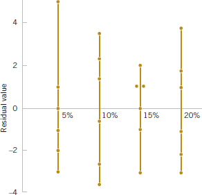
FIGURE 13-5 Plot of residuals versus factor levels (hardwood concentration).

FIGURE 13-6 Plot of residuals versus ![]() i.
i.
13-2.5 DETERMINING SAMPLE SIZE
In any experimental design problem, the choice of the sample size or number of replicates to use is important. Operating characteristic (OC) curves can be used to provide guidance here. Recall that an OC curve is a plot of the probability of a type II error (β) for various sample sizes against values of the parameters under test. The OC curves can be used to determine how many replicates are required to achieve adequate sensitivity.
The power of the ANOVA test is
![]()
To evaluate this probability statement, we need to know the distribution of the test statistic F0 if the null hypothesis is false. Because ANOVA compares several means, the null hypothesis can be false in different ways. For example, possibly τ1 > 0, τ2 = 0, τ3 < 0, and so forth. It can be shown that the power for ANOVA in Equation 13-17 depends on the τi's only through the function
![]()
Therefore, an alternative hypotheses for the τi's can be used to calculate Φ2 and this in turn can be used to calculate the power. Specifically, it can be shown that if H0 is false, the statistic F0 = MSTreatments/MSE has a noncentral F-distribution with a − 1 and n(a − 1) degrees of freedom and a noncentrality parameter that depends on Φ2. Instead of tables for the noncentral F-distribution, OC curves are used to evaluate β defined in Equation 13-17. These curves plot β against Φ.

FIGURE 13-7 Operating characteristic curves for the fixed-effects model analysis of variance. Top curves for four treatments and bottom curves for five treatments.
OC curves are available for α = 0.05 and α = 0.01 and for several values of the number of degrees of freedom for numerator (denoted v1) and denominator (denoted v2). Figure 13-7 gives representative OC curves, one for a = 4 (v1 = 3) and one for a = 5 (v1 = 4) treatments. Notice that for each value of a, there are curves for α = 0.05 and α = 0.01.
In using the curves, we must define the difference in means that we wish to detect in terms of ![]() . Also, the error variance σ2 is usually unknown. In such cases, we must choose ratios of
. Also, the error variance σ2 is usually unknown. In such cases, we must choose ratios of ![]() that we wish to detect. Alternatively, if an estimate of σ2 is available, one may replace σ2 with this estimate. For example, if we were interested in the sensitivity of an experiment that has already been performed, we might use MSE as the estimate of σ2.
that we wish to detect. Alternatively, if an estimate of σ2 is available, one may replace σ2 with this estimate. For example, if we were interested in the sensitivity of an experiment that has already been performed, we might use MSE as the estimate of σ2.
Example 13-3 Suppose that five means are being compared in a completely randomized experiment with α = 0.01. The experimenter would like to know how many replicates to run if it is important to reject H0 with probability at least 0.90 if ![]() . The parameter Φ2 is, in this case,
. The parameter Φ2 is, in this case,
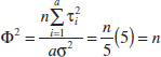
and for the OC curve with v1 = a − 1 = 5 − 1 = 4, and v2 = a(n − 1) = 5(n − 1) error degrees of freedom refer to the lower curve in Figure 13-7. As a first guess, try n = 4 replicates. This yields Φ2 = 4, Φ = 2, and v2 = 5(3) = 15 error degrees of freedom. Consequently, from Figure 13-7, we find that β ![]() 0.38. Therefore, the power of the test is approximately 1 − β = 1 − 0.38 = 0.62, which is less than the required 0.90, so we conclude that n = 4 replicates is not sufficient. Proceeding in a similar manner, we can construct the following table:
0.38. Therefore, the power of the test is approximately 1 − β = 1 − 0.38 = 0.62, which is less than the required 0.90, so we conclude that n = 4 replicates is not sufficient. Proceeding in a similar manner, we can construct the following table:
Conclusions: At least n = 6 replicates must be run in order to obtain a test with the required power.
Exercises FOR SECTION 13-2
![]() Problem available in WileyPLUS at instructor's discretion.
Problem available in WileyPLUS at instructor's discretion.
![]() Go Tutorial Tutoring problem available in WileyPLUS at instructor's discretion.
Go Tutorial Tutoring problem available in WileyPLUS at instructor's discretion.
13-1. Consider the following computer output.

(a) How many levels of the factor were used in this experiment?
(b) How many replicates did the experimenter use?
(c) Fill in the missing information in the ANOVA table. Use bounds for the P-value.
(d) What conclusions can you draw about differences in the factor-level means?
13-2. Consider the following computer output for an experiment. The factor was tested over four levels.

(a) How many replicates did the experimenter use?
(b) Fill in the missing information in the ANOVA table. Use bounds for the P-value.
(c) What conclusions can you draw about differences in the factor-level means?
13-3. Consider the following computer output for an experiment.

(a) How many replicates did the experimenter use?
(b) Fill in the missing information in the ANOVA table. Use bounds for the P-value.
(c) What conclusions can you draw about differences in the factor-level means?
(d) Compute an estimate for σ2.
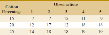
![]() 13-4. An article in Nature describes an experiment to investigate the effect on consuming chocolate on cardiovascular health (“Plasma Antioxidants from Chocolate,” 2003, Vol. 424, pp. 1013). The experiment consisted of using three different types of chocolates: 100 g of dark chocolate, 100 g of dark chocolate with 200 ml of full-fat milk, and 200 g of milk chocolate. Twelve subjects were used, seven women and five men with an average age range of 32.2±1 years, an average weight of 65.8±3.1 kg, and body-mass index of 21.9±0.4 kg m−2. On different days, a subject consumed one of the chocolate-factor levels, and one hour later total antioxidant capacity of that person's blood plasma was measured in an assay. Data similar to those summarized in the article follow.
13-4. An article in Nature describes an experiment to investigate the effect on consuming chocolate on cardiovascular health (“Plasma Antioxidants from Chocolate,” 2003, Vol. 424, pp. 1013). The experiment consisted of using three different types of chocolates: 100 g of dark chocolate, 100 g of dark chocolate with 200 ml of full-fat milk, and 200 g of milk chocolate. Twelve subjects were used, seven women and five men with an average age range of 32.2±1 years, an average weight of 65.8±3.1 kg, and body-mass index of 21.9±0.4 kg m−2. On different days, a subject consumed one of the chocolate-factor levels, and one hour later total antioxidant capacity of that person's blood plasma was measured in an assay. Data similar to those summarized in the article follow.
(a) Construct comparative box plots and study the data. What visual impression do you have from examining these plots?
(b) Analyze the experimental data using an ANOVA. If α = 0.05, what conclusions would you draw? What would you conclude if α = 0.01?
(c) Is there evidence that the dark chocolate increases the mean antioxidant capacity of the subjects' blood plasma?
(d) Analyze the residuals from this experiment.
![]() 13-5.
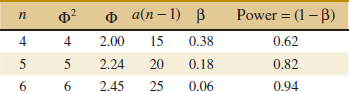
13-5. ![]() In Design and Analysis of Experiments, 8th edition (John Wiley & Sons, 2012), D. C. Montgomery described an experiment in which the tensile strength of a synthetic fiber was of interest to the manufacturer. It is suspected that strength is related to the percentage of cotton in the fiber. Five levels of cotton percentage were used, and five replicates were run in random order, resulting in the following data.
In Design and Analysis of Experiments, 8th edition (John Wiley & Sons, 2012), D. C. Montgomery described an experiment in which the tensile strength of a synthetic fiber was of interest to the manufacturer. It is suspected that strength is related to the percentage of cotton in the fiber. Five levels of cotton percentage were used, and five replicates were run in random order, resulting in the following data.
![]()
(a) Does cotton percentage affect breaking strength? Draw comparative box plots and perform an analysis of variance. Use α = 0.05.
(b) Plot average tensile strength against cotton percentage and interpret the results.
(c) Analyze the residuals and comment on model adequacy.
![]()
13-6. ![]() In “Orthogonal Design for Process Optimization and Its Application to Plasma Etching” (Solid State Technology, May 1987), G. Z. Yin and D. W. Jillie described an experiment to determine the effect of C2F6 flow rate on the uniformity of the etch on a silicon wafer used in integrated circuit manufacturing. Three flow rates are used in the experiment, and the resulting uniformity (in percent) for six replicates follows.
In “Orthogonal Design for Process Optimization and Its Application to Plasma Etching” (Solid State Technology, May 1987), G. Z. Yin and D. W. Jillie described an experiment to determine the effect of C2F6 flow rate on the uniformity of the etch on a silicon wafer used in integrated circuit manufacturing. Three flow rates are used in the experiment, and the resulting uniformity (in percent) for six replicates follows.

(a) Does C2F6 flow rate affect etch uniformity? Construct box plots to compare the factor levels and perform the analysis of variance. Use α = 0.05.
(b) Do the residuals indicate any problems with the underlying assumptions?
![]()
13-7. ![]() The compressive strength of concrete is being studied, and four different mixing techniques are being investigated. The following data have been collected.
The compressive strength of concrete is being studied, and four different mixing techniques are being investigated. The following data have been collected.
(a) Test the hypothesis that mixing techniques affect the strength of the concrete. Use α = 0.05.
(b) Find the P-value for the F-statistic computed in part (a).
(c) Analyze the residuals from this experiment.

![]()
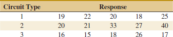
13-8. ![]() The response time in milliseconds was determined for three different types of circuits in an electronic calculator. The results are recorded here.
The response time in milliseconds was determined for three different types of circuits in an electronic calculator. The results are recorded here.
(a) Using α = 0.01, test the hypothesis that the three circuit types have the same response time.
(b) Analyze the residuals from this experiment.
(c) Find a 95% confidence interval on the response time for circuit 3.
![]() 13-9.
13-9. ![]() Go Tutorial An electronics engineer is interested in the effect on tube conductivity of five different types of coating for cathode ray tubes in a telecommunications system display device. The following conductivity data are obtained.
Go Tutorial An electronics engineer is interested in the effect on tube conductivity of five different types of coating for cathode ray tubes in a telecommunications system display device. The following conductivity data are obtained.

(a) Is there any difference in conductivity due to coating type? Use α = 0.01.
(b) Analyze the residuals from this experiment.
(c) Construct a 95% interval estimate of the coating type 1 mean. Construct a 99% interval estimate of the mean difference between coating types 1 and 4.
![]() 13-10. An article in Environment International [1992, Vol. 18(4)] described an experiment in which the amount of radon released in showers was investigated. Radon-enriched water was used in the experiment, and six different orifice diameters were tested in shower heads. The data from the experiment are shown in the following table.
13-10. An article in Environment International [1992, Vol. 18(4)] described an experiment in which the amount of radon released in showers was investigated. Radon-enriched water was used in the experiment, and six different orifice diameters were tested in shower heads. The data from the experiment are shown in the following table.

(a) Does the size of the orifice affect the mean percentage of radon released? Use α = 0.05.
(b) Find the P-value for the F-statistic in part (a).
(c) Analyze the residuals from this experiment.
(d) Find a 95% confidence interval on the mean percent of radon released when the orifice diameter is 1.40.
![]() 13-11.
13-11. ![]() An article in the ACI Materials Journal (1987, Vol. 84, pp. 213–216) described several experiments investigating the rodding of concrete to remove entrapped air. A 3-inch × 6-inch cylinder was used, and the number of times this rod was used is the design variable. The resulting compressive strength of the concrete specimen is the response. The data are shown in the following table.
An article in the ACI Materials Journal (1987, Vol. 84, pp. 213–216) described several experiments investigating the rodding of concrete to remove entrapped air. A 3-inch × 6-inch cylinder was used, and the number of times this rod was used is the design variable. The resulting compressive strength of the concrete specimen is the response. The data are shown in the following table.

(a) Is there any difference in compressive strength due to the rodding level?
(b) Find the P-value for the F-statistic in part (a).
(c) Analyze the residuals from this experiment. What conclusions can you draw about the underlying model assumptions?
![]()
13-12. An article in the Materials Research Bulletin [1991, Vol. 26(11)] investigated four different methods of preparing the superconducting compound PbMo6S8. The authors contend that the presence of oxygen during the preparation process affects the material's superconducting transition temperature Tc. Preparation methods 1 and 2 use techniques that are designed to eliminate the presence of oxygen, and methods 3 and 4 allow oxygen to be present. Five observations on Tc (in °K) were made for each method, and the results are as follows:

(a) Is there evidence to support the claim that the presence of oxygen during preparation affects the mean transition temperature? Use α = 0.05.
(b) What is the P-value for the F-test in part (a)?
(c) Analyze the residuals from this experiment.
(d) Find a 95% confidence interval on mean Tc when method 1 is used to prepare the material.
![]()
13-13. A paper in the Journal of the Association of Asphalt Paving Technologists (1990, Vol. 59) described an experiment to determine the effect of air voids on percentage retained strength of asphalt. For purposes of the experiment, air voids are controlled at three levels; low (2–4%), medium (4–6%), and high (6–8%). The data are shown in the following table.

(a) Do the different levels of air voids significantly affect mean retained strength? Use α = 0.01.
(b) Find the P-value for the F-statistic in part (a).
(c) Analyze the residuals from this experiment.
(d) Find a 95% confidence interval on mean retained strength where there is a high level of air voids.
(e) Find a 95% confidence interval on the difference in mean retained strength at the low and high levels of air voids.
![]()
13-14. An article in Quality Engineering [“Estimating Sources of Variation: A Case Study from Polyurethane Product Research” (1999–2000, Vol. 12, pp. 89–96)] reported a study on the effects of additives on final polymer properties. In this case, polyurethane additives were referred to as cross-linkers. The average domain spacing was the measurement of the polymer property. The data are as follows:

(a) Is there a difference in the cross-linker level? Draw comparative box plots and perform an analysis of variance. Use α = 0.05.
(b) Find the P-value of the test. Estimate the variability due to random error.
(c) Plot average domain spacing against cross-linker level and interpret the results.
(d) Analyze the residuals from this experiment and comment on model adequacy.
![]() 13-15. In the book Analysis of Longitudinal Data, 2nd ed., (2002, Oxford University Press), by Diggle, Heagerty, Liang, and Zeger, the authors analyzed the effects of three diets on the protein content of cow's milk. The data shown here were collected after one week and include 25 cows on the barley diet and 27 cows each on the other two diets:
13-15. In the book Analysis of Longitudinal Data, 2nd ed., (2002, Oxford University Press), by Diggle, Heagerty, Liang, and Zeger, the authors analyzed the effects of three diets on the protein content of cow's milk. The data shown here were collected after one week and include 25 cows on the barley diet and 27 cows each on the other two diets:

(a) Does diet affect the protein content of cow's milk? Draw comparative box plots and perform an analysis of variance. Use α = 0.05.
(b) Find the P-value of the test. Estimate the variability due to random error.
(c) Plot average protein content against diets and interpret the results.
(d) Analyze the residuals and comment on model adequacy.
![]() 13-16.
13-16. ![]() An article in Journal of Food Science [2001, Vol. 66(3), pp. 472–477] reported on a study of potato spoilage based on different conditions of acidified oxine (AO), which is a mixture of chlorite and chlorine dioxide. The data follow:
An article in Journal of Food Science [2001, Vol. 66(3), pp. 472–477] reported on a study of potato spoilage based on different conditions of acidified oxine (AO), which is a mixture of chlorite and chlorine dioxide. The data follow:
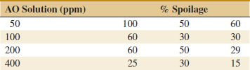
(a) Do the AO solutions differ in the spoilage percentage? Use α = 0.05.
(b) Find the P-value of the test. Estimate the variability due to random error.
(c) Plot average spoilage against AO solution and interpret the results. Which AO solution would you recommend for use in practice?
(d) Analyze the residuals from this experiment.
![]()
13-17. ![]() An experiment was run to determine whether four specific firing temperatures affect the density of a certain type of brick. The experiment led to the following data.
An experiment was run to determine whether four specific firing temperatures affect the density of a certain type of brick. The experiment led to the following data.
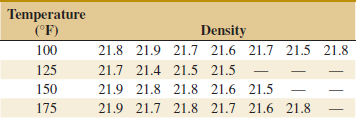
(a) Does the firing temperature affect the density of the bricks? Use α = 0.05.
(b) Find the P-value for the F-statistic computed in part (a).
(c) Analyze the residuals from the experiment.
![]()
13-18. An article in Scientia Iranica [“Tuning the Parameters of an Artificial Neural Network (ANN) Using Central Composite Design and Genetic Algorithm” (2011, Vol. 18(6), pp. 1600–608)], described a series of experiments to tune parameters in artificial neural networks. One experiment considered the relationship between model fitness [measured by the square root of mean square error (RMSE) on a separate test set of data] and model complexity that were controlled by the number of nodes in the two hidden layers. The following data table (extracted from a much larger data set) contains three different ANNs: ANN1 has 33 nodes in layer 1 and 30 nodes in layer 2, ANN2 has 49 nodes in layer 1 and 45 nodes in layer 2, and ANN3 has 17 nodes in layer 1 and 15 nodes in layer 2.

(a) Construct a box plot to compare the different ANNs.
(b) Perform the analysis of variance with α = 0.05. What is the P-value?
(c) Analyze the residuals from the experiment.
(d) Calculate a 95% confidence interval on RMSE for ANN2.
![]() 13-19. An article in Fuel Processing Technology (“Application of the Factorial Design of Experiments to Biodiesel Production from Lard,” 2009, Vol. 90, pp. 1447–1451) described an experiment to investigate the effect of potassium hydroxide in synthesis of biodiesel. It is suspected that potassium hydroxide (PH) is related to fatty acid methyl esters (FAME) which are key elements in biodiesel. Three levels of PH concentration were used, and six replicates were run in a random order. Data are shown in the following table.
13-19. An article in Fuel Processing Technology (“Application of the Factorial Design of Experiments to Biodiesel Production from Lard,” 2009, Vol. 90, pp. 1447–1451) described an experiment to investigate the effect of potassium hydroxide in synthesis of biodiesel. It is suspected that potassium hydroxide (PH) is related to fatty acid methyl esters (FAME) which are key elements in biodiesel. Three levels of PH concentration were used, and six replicates were run in a random order. Data are shown in the following table.
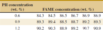
(a) Construct box plots to compare the factor levels.
(b) Construct the analysis of variance. Are there any differences in PH concentrations at α = 0.05? Calculate the P-value.
(c) Analyze the residuals from the experiment.
(d) Plot average FAME against PH concentration and interpret your results.
(e) Compute a 95% confidence interval on mean FAME when the PH concentration is 1.2.
For each of the following exercises, use the previous data to complete these parts.
(a) Apply Fisher's LSD method with α = 0.05 and determine which levels of the factor differ.
(b) Use the graphical method to compare means described in this section and compare your conclusions to those from Fisher's LSD method.
![]()
13-20. Chocolate type in Exercise 13-4. Use α = 0.05.
![]()
13-21. Cotton percentage in Exercise 13-5. Use α = 0.05.
![]()
13-22. ![]() Flow rate in Exercise 13-6. Use α = 0.01.
Flow rate in Exercise 13-6. Use α = 0.01.
![]()
13-23. ![]() Mixing technique in Exercise 13-7. Use α = 0.05.
Mixing technique in Exercise 13-7. Use α = 0.05.
![]()
13-24. Circuit type in Exercise 13-8. Use α = 0.01.
![]()
13-25. Coating type in Exercise 13-9. Use α = 0.01.
![]()
13-26. Preparation method in Exercise 13-12. Use α = 0.05.
![]()
13-27. Air voids in Exercise 13-13. Use α = 0.05.
![]()
13-28. Cross-linker Exercise 13-14. Use α = 0.05.
![]()
13-29. Diets in Exercise 13-15. Use α = 0.01.
![]()
13-30. ![]() Suppose that four normal populations have common variance σ2 = 25 and means μ1 = 50, μ2 = 60, μ3 = 50, and μ4 = 60. How many observations should be taken on each population so that the probability of rejecting the hypothesis of equality of means is at least 0.90? Use α = 0.05.
Suppose that four normal populations have common variance σ2 = 25 and means μ1 = 50, μ2 = 60, μ3 = 50, and μ4 = 60. How many observations should be taken on each population so that the probability of rejecting the hypothesis of equality of means is at least 0.90? Use α = 0.05.
13-31. Suppose that five normal populations have common variance σ2 = 100 and means μ1 = 175, μ2 = 190, μ3 = 160, μ4 = 200, and μ5 = 215. How many observations per population must be taken so that the probability of rejecting the hypothesis of equality of means is at least 0.95? Use α = 0.01.
13-32. ![]() Suppose that four normal populations with common variance σ2 are to be compared with a sample size of eight observations from each population. Determine the smallest value for
Suppose that four normal populations with common variance σ2 are to be compared with a sample size of eight observations from each population. Determine the smallest value for ![]() that can be detected with power 90%. Use α = 0.05.
that can be detected with power 90%. Use α = 0.05.
13-33. Suppose that five normal populations with common variance σ2 are to be compared with a sample size of seven observations from each. Suppose that τ1 = ··· = τ4 = 0. What is the smallest value for ![]() /σ2 that can be detected with power 90% and α = 0.01?
/σ2 that can be detected with power 90% and α = 0.01?
13-3 The Random-Effects Model
13-3.1 FIXED VERSUS RANDOM FACTORS
In many situations, the factor of interest has a large number of possible levels. The analyst is interested in drawing conclusions about the entire population of factor levels. If the experimenter randomly selects a of these levels from the population of factor levels, we say that the factor is a random factor. Because the levels of the factor actually used in the experiment are chosen randomly, the conclusions reached are valid for the entire population of factor levels. We assume that the population of factor levels is either of infinite size or is large enough to be considered infinite. Notice that this is a very different situation than the one we encountered in the fixed-effects case in which the conclusions apply only for the factor levels used in the experiment.
13-3.2 ANOVA AND VARIANCE COMPONENTS
The linear statistical model is
![]()
where the treatment effects τi and the errors εij are independent random variables. Note that the model is identical in structure to the fixed-effects case, but the parameters have a different interpretation. If the variance of the treatment effects τi is ![]() , by independence the variance of the response is
, by independence the variance of the response is
![]()
The variances ![]() and σ2 are called variance components, and the model, Equation 13-19, is called the components of variance model or the random-effects model. To test hypotheses in this model, we assume that the errors
and σ2 are called variance components, and the model, Equation 13-19, is called the components of variance model or the random-effects model. To test hypotheses in this model, we assume that the errors ![]() ij are normally and independently distributed with mean zero and variance σ2 and that the treatment effects τi are normally and independently distributed with mean zero and variance
ij are normally and independently distributed with mean zero and variance σ2 and that the treatment effects τi are normally and independently distributed with mean zero and variance ![]() .*
.*
For the random-effects model, testing the hypothesis that the individual treatment effects are zero is meaningless. It is more appropriate to test hypotheses about ![]() . Specifically,
. Specifically,
![]()
If ![]() = 0, all treatments are identical; but if
= 0, all treatments are identical; but if ![]() > 0, there is variability between treatments.
> 0, there is variability between treatments.
The ANOVA decomposition of total variability is still valid; that is,
![]()
However, the expected values of the mean squares for treatments and error are somewhat different than in the fixed-effects case.
Expected Values of Mean Squares: Random Effects
In the random-effects model for a single-factor, completely randomized experiment, the expected mean square for treatments is
![]()
and the expected mean square for error is
![]()
From examining the expected mean squares, it is clear that both MSE and MSTreatments estimate σ2 when H0: ![]() = 0 is true. Furthermore, MSE and MSTreatments are independent. Consequently, the ratio
= 0 is true. Furthermore, MSE and MSTreatments are independent. Consequently, the ratio
![]()
is an F random variable with a − 1 and a(n − 1) degrees of freedom when H0 is true. The null hypothesis would be rejected at the a-level of significance if the computed value of the test statistic f0 > fα,a−1,a(n−1).
The computational procedure and construction of the ANOVA table for the random-effects model are identical to the fixed-effects case. The conclusions, however, are quite different because they apply to the entire population of treatments.
Usually, we also want to estimate the variance components (σ2 and ![]() ) in the model. The procedure that we use to estimate σ2 and
) in the model. The procedure that we use to estimate σ2 and ![]() is called the analysis of variance method because it uses the information in the analysis of variance table. It does not require the normality assumption on the observations. The procedure consists of equating the expected mean squares to their observed values in the ANOVA table and solving for the variance components. When equating observed and expected mean squares in the one-way classification random-effects model, we obtain
is called the analysis of variance method because it uses the information in the analysis of variance table. It does not require the normality assumption on the observations. The procedure consists of equating the expected mean squares to their observed values in the ANOVA table and solving for the variance components. When equating observed and expected mean squares in the one-way classification random-effects model, we obtain
![]()
Therefore, the estimators of the variance components are
ANOVA Variance Components Estimates
![]()
and
![]()
Sometimes the analysis of variance method produces a negative estimate of a variance component. Because variance components are by definition non-negative, a negative estimate of a variance component is disturbing. One course of action is to accept the estimate and use it as evidence that the true value of the variance component is zero, assuming that sampling variation led to the negative estimate. Although this approach has intuitive appeal, it will disturb the statistical properties of other estimates. Another alternative is to reestimate the negative variance component with a method that always yields non-negative estimates. Still another possibility is to consider the negative estimate as evidence that the assumed linear model is incorrect, requiring that a study of the model and its assumptions be made to find a more appropriate model.
Example 13-4 Textile Manufacturing In Design and Analysis of Experiments, 8th edition (John Wiley, 2012), D. C. Montgomery describes a single-factor experiment involving the random-effects model in which a textile manufacturing company weaves a fabric on a large number of looms. The company is interested in loom-to-loom variability in tensile strength. To investigate this variability, a manufacturing engineer selects four looms at random and makes four strength determinations on fabric samples chosen at random from each loom. The data are shown in Table 13-7 and the ANOVA is summarized in Table 13-8.
![]() TABLE • 13-7 Strength Data for Example 13-4
TABLE • 13-7 Strength Data for Example 13-4

![]() TABLE • 13-8 Analysis of Variance for the Strength Data
TABLE • 13-8 Analysis of Variance for the Strength Data
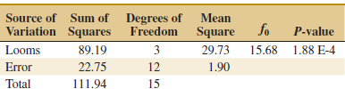
From the analysis of variance, we conclude that the looms in the plant differ significantly in their ability to produce fabric of uniform strength. The variance components are estimated by ![]() 2 = 1.90 and
2 = 1.90 and
![]()
Therefore, the variance of strength in the manufacturing process is estimated by
![]()
Conclusion: Most of the variability in strength in the output product is attributable to differences between looms.
This example illustrates an important application of the analysis of variance—the isolation of different sources of variability in a manufacturing process. Problems of excessive variability in critical functional parameters or properties frequently arise in quality-improvement programs. For example, in the previous fabric strength example, the process mean is estimated by ![]() = 95.45 psi, and the process standard deviation is estimated by
= 95.45 psi, and the process standard deviation is estimated by ![]() y =
y = ![]() =
= ![]() = 2.98 psi. If strength is approximately normally distributed, the distribution of strength in the outgoing product would look like the normal distribution shown in Fig. 13-8(a). If the lower specification limit (LSL) on strength is at 90 psi, a substantial proportion of the process output is fallout—that is, scrap or defective material that must be sold as second quality, and so on. This fallout is directly related to the excess variability resulting from differences between looms. Variability in loom performance could be caused by faulty setup, poor maintenance, inadequate supervision, poorly trained operators, and so forth. The engineer or manager responsible for quality improvement must identify and remove these sources of variability from the process. If this can be done, strength variability will be greatly reduced, perhaps as low as
= 2.98 psi. If strength is approximately normally distributed, the distribution of strength in the outgoing product would look like the normal distribution shown in Fig. 13-8(a). If the lower specification limit (LSL) on strength is at 90 psi, a substantial proportion of the process output is fallout—that is, scrap or defective material that must be sold as second quality, and so on. This fallout is directly related to the excess variability resulting from differences between looms. Variability in loom performance could be caused by faulty setup, poor maintenance, inadequate supervision, poorly trained operators, and so forth. The engineer or manager responsible for quality improvement must identify and remove these sources of variability from the process. If this can be done, strength variability will be greatly reduced, perhaps as low as ![]() Y =
Y = ![]() =
= ![]() = 1.38 psi, as shown in Fig. 13-8(b). In this improved process, reducing the variability in strength has greatly reduced the fallout, resulting in lower cost, higher quality, a more satisfied customer, and an enhanced competitive position for the company.
= 1.38 psi, as shown in Fig. 13-8(b). In this improved process, reducing the variability in strength has greatly reduced the fallout, resulting in lower cost, higher quality, a more satisfied customer, and an enhanced competitive position for the company.

FIGURE 13-8 The distribution of fabric strength. (a) Current process, (b) Improved process.
Exercises FOR SECTION 13-3
![]() Problem available in WileyPLUS at instructor's discretion.
Problem available in WileyPLUS at instructor's discretion.
![]() Go Tutorial Tutoring problem available in WileyPLUS at instructor's discretion.
Go Tutorial Tutoring problem available in WileyPLUS at instructor's discretion.
![]() 13-34.
13-34. ![]() An article in the Journal of the Electrochemical Society [1992, Vol. 139(2), pp. 524–532)] describes an experiment to investigate the low-pressure vapor deposition of polysilicon. The experiment was carried out in a large-capacity reactor at Sematech in Austin, Texas. The reactor has several wafer positions, and four of these positions were selected at random. The response variable is film thickness uniformity. Three replicates of the experiment were run, and the data are as follows:
An article in the Journal of the Electrochemical Society [1992, Vol. 139(2), pp. 524–532)] describes an experiment to investigate the low-pressure vapor deposition of polysilicon. The experiment was carried out in a large-capacity reactor at Sematech in Austin, Texas. The reactor has several wafer positions, and four of these positions were selected at random. The response variable is film thickness uniformity. Three replicates of the experiment were run, and the data are as follows:
(a) Is there a difference in the wafer positions? Use α = 0.05.
(b) Estimate the variability due to wafer positions.
(c) Estimate the random error component.
(d) Analyze the residuals from this experiment and comment on model adequacy.

![]()
13-35. ![]() A textile mill has a large number of looms. Each loom is supposed to provide the same output of cloth per minute. To investigate this assumption, five looms are chosen at random, and their output is measured at different times. The following data are obtained:
A textile mill has a large number of looms. Each loom is supposed to provide the same output of cloth per minute. To investigate this assumption, five looms are chosen at random, and their output is measured at different times. The following data are obtained:

(a) Are the looms similar in output? Use α = 0.05.
(b) Estimate the variability between looms.
(c) Estimate the experimental error variance.
(d) Analyze the residuals from this experiment and check for model adequacy.
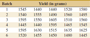
![]() 13-36. In the book Bayesian Inference in Statistical Analysis (1973, John Wiley and Sons) by Box and Tiao, the total product yield for five samples was determined randomly selected from each of six randomly chosen batches of raw material.
13-36. In the book Bayesian Inference in Statistical Analysis (1973, John Wiley and Sons) by Box and Tiao, the total product yield for five samples was determined randomly selected from each of six randomly chosen batches of raw material.
(a) Do the different batches of raw material significantly affect mean yield? Use α = 0.01.
(b) Estimate the variability between batches.
(c) Estimate the variability between samples within batches.
(d) Analyze the residuals from this experiment and check for model adequacy.
![]() 13-37.
13-37. ![]() An article in the Journal of Quality Technology [1981, Vol. 13(2), pp. 111–114)] described an experiment that investigated the effects of four bleaching chemicals on pulp brightness. These four chemicals were selected at random from a large population of potential bleaching agents. The data are as follows:
An article in the Journal of Quality Technology [1981, Vol. 13(2), pp. 111–114)] described an experiment that investigated the effects of four bleaching chemicals on pulp brightness. These four chemicals were selected at random from a large population of potential bleaching agents. The data are as follows:
(a) Is there a difference in the chemical types? Use α = 0.05.
(b) Estimate the variability due to chemical types.
(c) Estimate the variability due to random error.
(d) Analyze the residuals from this experiment and comment on model adequacy.

![]()
13-38. ![]() Consider the vapor-deposition experiment described in Exercise 13-34.
Consider the vapor-deposition experiment described in Exercise 13-34.
(a) Estimate the total variability in the uniformity response.
(b) How much of the total variability in the uniformity response is due to the difference between positions in the reactor?
(c) To what level could the variability in the uniformity response be reduced if the position-to-position variability in the reactor could be eliminated? Do you believe this is a substantial reduction?
![]()
13-39. Consider the cloth experiment described in Exercise 13-35.
(a) Estimate the total variability in the output response.
(b) How much of the total variability in the output response is due to the difference between looms?
(c) To what level could the variability in the output response be reduced if the loom-to-loom variability could be eliminated? Do you believe this is a significant reduction?
![]()
13-40. Reconsider Exercise 13-8 in which the effect of different circuits on the response time was investigated. Suppose that the three circuits were selected at random from a large number of circuits.
(a) How does this change the interpretation of the experiment?
(b) What is an appropriate statistical model for this experiment?
(c) Estimate the parameters of this model.
![]()
13-41. Reconsider Exercise 13-15 in which the effect of different diets on the protein content of cow's milk was investigated. Suppose that the three diets reported were selected at random from a large number of diets. To simplify, delete the last two observations in the diets with n = 27 (to make equal sample sizes).
(a) How does this change the interpretation of the experiment?
(b) What is an appropriate statistical model for this experiment?
(c) Estimate the parameters of this model.
13-4 Randomized Complete Block Design
13-4.1 DESIGN AND STATISTICAL ANALYSIS
In many experimental design problems, it is necessary to design the experiment so that the variability arising from a nuisance factor can be controlled. For example, consider the situation of Example 10-10 in which two different methods were used to predict the shear strength of steel plate girders. Because each girder has different strength (potentially), and this variability in strength was not of direct interest, we designed the experiment by using the two test methods on each girder and then comparing the average difference in strength readings on each girder to zero using the paired t-test. The paired t-test is a procedure for comparing two treatment means when all experimental runs cannot be made under homogeneous conditions. Alternatively, we can view the paired t-test as a method for reducing the background noise in the experiment by blocking out a nuisance factor effect. The block is the nuisance factor, and in this case, the nuisance factor is the actual experimental unit—the steel girder specimens used in the experiment.
The randomized block design is an extension of the paired t-test to situations where the factor of interest has more than two levels; that is, more than two treatments must be compared. For example, suppose that three methods could be used to evaluate the strength readings on steel plate girders. We may think of these as three treatments, say t1, t2, and t3. If we use four girders as the experimental units, a randomized complete block design (RCBD) would appear as shown in Fig. 13-9. The design is called a RCBD because each block is large enough to hold all the treatments and because the actual assignment of each of the three treatments within each block is done randomly. Once the experiment has been conducted, the data are recorded in a table, such as is shown in Table 13-9. The observations in this table, say, yij, represent the response obtained when method i is used on girder j.
The general procedure for a RCBD consists of selecting b blocks and running a complete replicate of the experiment in each block. The data that result from running a RCBD for investigating a single factor with a levels and b blocks are shown in Table 13-10. There are a observations (one per factor level) in each block, and the order in which these observations are run is randomly assigned within the block.
We now describe the statistical analysis for the RCBD. Suppose that a single factor with a levels is of interest and that the experiment is run in b blocks. The observations may be represented by the linear statistical model
![]()
where μ is an overall mean, τi is the effect of the ith treatment, βj is the effect of the jth block, and ![]() ij is the random error term, which is assumed to be normally and independently distributed with mean zero and variance σ2. Furthermore, the treatment and block effects are defined as deviations from the overall mean, so
ij is the random error term, which is assumed to be normally and independently distributed with mean zero and variance σ2. Furthermore, the treatment and block effects are defined as deviations from the overall mean, so ![]() and
and ![]() . This was the same type of definition used for completely randomized experiments in Section 13-2. We also assume that treatments and blocks do not interact. That is, the effect of treatment i is the same regardless of which block (or blocks) in which it is tested. We are interested in testing the equality of the treatment effects. That is,
. This was the same type of definition used for completely randomized experiments in Section 13-2. We also assume that treatments and blocks do not interact. That is, the effect of treatment i is the same regardless of which block (or blocks) in which it is tested. We are interested in testing the equality of the treatment effects. That is,
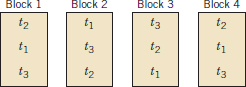
FIGURE 13-9 A randomized complete block design.
![]() TABLE • 13-9 A Randomized Complete Block Design
TABLE • 13-9 A Randomized Complete Block Design

![]() TABLE • 13-10 A Randomized Complete Block Design with a Treatments and b Blocks
TABLE • 13-10 A Randomized Complete Block Design with a Treatments and b Blocks
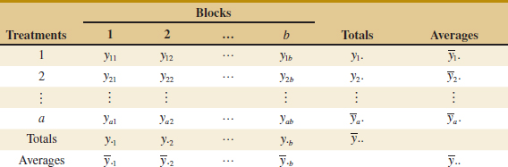
The analysis of variance can be extended to the RCBD. The procedure uses a sum of squares identity that partitions the total sum of squares into three components.
ANOVA Sums of Squares Identity: Randomized Complete Block Experiment
The sum of squares identity for the randomized complete block design is

or symbolically
![]()
Furthermore, the degrees of freedom corresponding to these sums of squares are
![]()
For the randomized block design, the relevant mean squares are
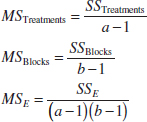
The expected values of these mean squares can be shown to be as follows:
Expected Mean Squares: Randomized Complete Block Experiment

Therefore, if the null hypothesis H0 is true so that all treatment effects τi = 0, MSTreatments is an unbiased estimator of σ2, and if H0 is false, MSTreatments overestimates σ2. The mean square for error is always an unbiased estimate of σ2. To test the null hypothesis that the treatment effects are all zero, we use the ratio
![]()
which has an F-distribution with a − 1 and (a − 1)(b − 1) degrees of freedom if the null hypothesis is true. We would reject the null hypothesis at the a-level of significance if the computed value of the test statistic in Equation 13-28 is f0 > fα,a−1,(a−1)(b−1).
In practice, we compute SST, SSTreatments and SSBlocks and then obtain the error sum of squares SSE by subtraction. The appropriate computing formulas are as follows.
The computing formulas for the sums of squares in the analysis of variance for a RCBD are

and
![]()
The computations are usually arranged in an ANOVA table, such as is shown in Table 13-11. Generally, computer software is used to perform the analysis of variance for a RCBD.
![]() TABLE • 13-11 ANOVA for a Randomized Complete Block Design
TABLE • 13-11 ANOVA for a Randomized Complete Block Design

Example 13-5 Fabric Strength An experiment was performed to determine the effect of four different chemicals on the strength of a fabric. These chemicals are used as part of the permanent press finishing process. Five fabric samples were selected, and a RCBD was run by testing each chemical type once in random order on each fabric sample. The data are shown in Table 13-12. We test for differences in means using an ANOVA with α = 0.01.
The sums of squares for the analysis of variance are computed as follows:
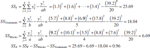
The ANOVA is summarized in Table 13-13. Because f0 = 75.13 > f0.01,3,12 = 5.95 (the P-value is 4.79 × 10⁻⁸ from computer software), we conclude that there is a significant difference in the chemical types so far as their effect on strength is concerned.
![]() TABLE • 13-12 Fabric Strength Data—Randomized Complete Block Design
TABLE • 13-12 Fabric Strength Data—Randomized Complete Block Design

When Is Blocking Necessary?
Suppose that an experiment is conducted as a RCBD and blocking was not really necessary. There are ab observations and (a − 1)(b − 1) degrees of freedom for error. If the experiment had been run as a completely randomized single-factor design with b replicates, we would have had a(b − 1) degrees of freedom for error. Therefore, blocking has cost a(b − 1) − (a − 1)(b − 1) = b − 1 degrees of freedom for error. This loss in degrees of freedom increases the critical value from the F-distribution in Equation 13-28. Consequently, to detect a treatment effect, greater differences in treatment means are needed. However, because the loss in error degrees of freedom is usually small, if there is a reasonable chance that block effects may be important, the experimenter should use the RCBD.
For example, consider the experiment described in Example 13-5 as a single-factor experiment with no blocking. We would then have 16 degrees of freedom for error. In the RCBD, there are 12 degrees of freedom for error. Therefore, blocking has cost only 4 degrees of freedom, which is a very small loss considering the possible gain in information that would be achieved if block effects are really important. The block effect in Example 13-5 is large, and if we had not blocked, SSBlocks would have been included in the error sum of squares for the completely randomized analysis. This would have resulted in a much larger MSE, making it more difficult to detect treatment differences. As a general rule, when in doubt as to the importance of block effects, the experimenter should block and gamble that the block effect does exist. If the experimenter is wrong, the slight loss in the degrees of freedom for error will have a negligible effect unless the number of degrees of freedom is very small.
Computer Solution
Table 13-14 presents computer output for the RCBD in Example 13-5. The results agree closely with the hand calculations from Table 13-13.
Notice that the software computes an F-statistic for the blocks (the fabric samples). The validity of this ratio as a test statistic for the null hypothesis of no block effects is doubtful because the blocks represent a restriction on randomization; that is, we have only randomized within the blocks. If the blocks are not chosen at random, or if they are not run in random order, the F-ratio for blocks may not provide reliable information about block effects. For more discussion see Montgomery (2012).
![]() TABLE • 13-13 Analysis of Variance for the Randomized Complete Block Experiment
TABLE • 13-13 Analysis of Variance for the Randomized Complete Block Experiment

13-4.2 MULTIPLE COMPARISONS
When the ANOVA indicates that a difference for the treatment means exists the treatment means, we may need to perform some follow-up tests to isolate the specific differences. Any multiple comparison method, such as Fisher's LSD method, could be used for this purpose.
Table 13-14 Computer Output for the Randomized Complete Block Design in Example 13-5
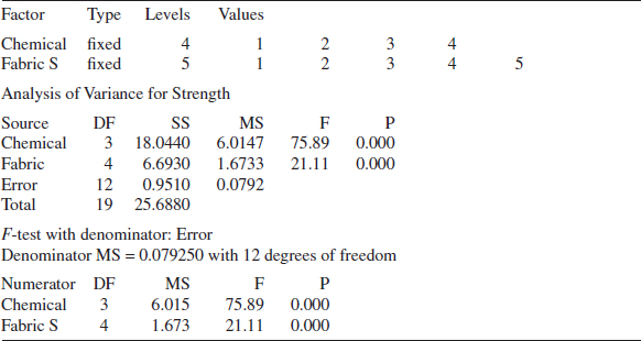
We illustrate Fisher's LSD method. The four chemical type averages from Example 13-5 are:
![]()
Each treatment average uses b = 5 observations (one from each block). We use α = 0.05, so t0.025,12 = 2.179. Therefore, the value of the LSD is
![]()
Any pair of treatment averages that differ by 0.39 or more indicates that this pair of treatment means is significantly different. The comparisons follow:
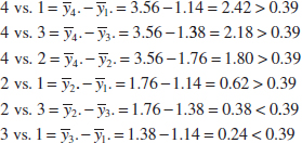
Figure 13-10 presents the results graphically. The underlined pairs of means are not different. The LSD procedure indicates that chemical type 4 results in significantly different strengths than the other three types do. Chemical types 2 and 3 do not differ, and types 1 and 3 do not differ. There may be a small difference in strength for types 1 and 2.

FIGURE 13-10 Results of Fisher's LSD method.
13-4.3 RESIDUAL ANALYSIS AND MODEL CHECKING
In any designed experiment, it is always important to examine the residuals and to check for violation of basic assumptions that could invalidate the results. As usual, the residuals for the RCBD are simply the differences in the observed and estimated (or fitted) values from the statistical model,
![]()
and the fitted values are
![]()
The fitted value represents the estimate of the mean response when the ith treatment is run in the jth block. The residuals from the chemical type experiment are shown in Table 13-15.
Figures 13-11, 13-12, 13-13, and 13-14 present the important residual plots for the experiment. These residual plots are usually constructed by computer software. When treated with the four chemicals, there is some indication that fabric sample (block) 3 has greater variability in strength than the other samples. Chemical type 4, which provides the greatest strength, also has somewhat more variability in strength. Follow-up experiments may be necessary to confirm these findings if they are potentially important.

FIGURE 13-11 Normal probability plot of residuals from the randomized complete block design.

FIGURE 13-12 Residuals by treatment from the randomized complete block design.

FIGURE 13-13 Residuals by block from the randomized complete block design.

FIGURE 13-14 Residuals versus ![]() ij from the randomized complete block design.
ij from the randomized complete block design.
![]() TABLE • 13-15 Residuals from the Randomized Complete Block Design
TABLE • 13-15 Residuals from the Randomized Complete Block Design

EXERCISES FOR SECTION 13-4
![]() Problem available in WileyPLUS at instructor's discretion.
Problem available in WileyPLUS at instructor's discretion.
![]() Go Tutorial Tutoring problem available in WileyPLUS at instructor's discretion.
Go Tutorial Tutoring problem available in WileyPLUS at instructor's discretion.
13-42. Consider the following computer output from a RCBD.

(a) How many levels of the factor were used in this experiment?
(b) How many blocks were used in this experiment?
(c) Fill in the missing information. Use bounds for the P-value.
(d) What conclusions would you draw if α = 0.05? What would you conclude if α = 0.01?
13-43. Consider the following computer output from a RCBD. There are four levels of the factor and five blocks.
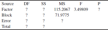
(a) Fill in the missing information. Use bounds for the P-value.
(b) What conclusions would you draw if α = 0.05? What would you conclude if α = 0.01?
![]() 13-44. Exercise 13-4 introduced you to an experiment to investigate the potential effect of consuming chocolate on cardiovascular health. The experiment was conducted as a completely randomized design, and the exercise asked you to use the ANOVA to analyze the data and draw conclusions. Now assume that the experiment had been conducted as an RCBD with the subjects considered as blocks. Analyze the data using this assumption. What conclusions would you draw (using α = 0.05) about the effect of the different types of chocolate on cardiovascular health? Would your conclusions change if α = 0.01?
13-44. Exercise 13-4 introduced you to an experiment to investigate the potential effect of consuming chocolate on cardiovascular health. The experiment was conducted as a completely randomized design, and the exercise asked you to use the ANOVA to analyze the data and draw conclusions. Now assume that the experiment had been conducted as an RCBD with the subjects considered as blocks. Analyze the data using this assumption. What conclusions would you draw (using α = 0.05) about the effect of the different types of chocolate on cardiovascular health? Would your conclusions change if α = 0.01?
![]() 13-45. Reconsider the experiment of Exercise 13-5. Suppose that the experiment was conducted as a RCBD with blocks formed by days (denoted as columns in the data table). In the experiment, the primary interest is still in the effect of cotton percentage and day is considered a nuisance factor.
13-45. Reconsider the experiment of Exercise 13-5. Suppose that the experiment was conducted as a RCBD with blocks formed by days (denoted as columns in the data table). In the experiment, the primary interest is still in the effect of cotton percentage and day is considered a nuisance factor.
(a) Consider day as a block, and re-estimate the ANOVA.
(b) Does cotton percentage still affect strength at α = 0.05?
(c) Compare the conclusions here with those obtained from the analysis without blocks.
![]()
13-46. ![]() An article in Quality Engineering [“Designed Experiment to Stabilize Blood Glucose Levels” (1999–2000, Vol. 12, pp. 83–87)] described an experiment to minimize variations in blood glucose levels. The treatment was the exercise time on a Nordic Track cross-country skier (10 or 20 min). The experiment was blocked for time of day. The data were as follows:
An article in Quality Engineering [“Designed Experiment to Stabilize Blood Glucose Levels” (1999–2000, Vol. 12, pp. 83–87)] described an experiment to minimize variations in blood glucose levels. The treatment was the exercise time on a Nordic Track cross-country skier (10 or 20 min). The experiment was blocked for time of day. The data were as follows:

(a) Is there an effect of exercise time on the average blood glucose? Use α = 0.05.
(b) Find the P-value for the test in part (a).
(c) Analyze the residuals from this experiment.
![]()
13-47. ![]() In “The Effect of Nozzle Design on the Stability and Performance of Turbulent Water Jets” (Fire Safety Journal, August 1981, Vol. 4), C. Theobald described an experiment in which a shape measurement was determined for several different nozzle types at different levels of jet efflux velocity. Interest in this experiment focuses primarily on nozzle type, and velocity is a nuisance factor. The data are as follows:
In “The Effect of Nozzle Design on the Stability and Performance of Turbulent Water Jets” (Fire Safety Journal, August 1981, Vol. 4), C. Theobald described an experiment in which a shape measurement was determined for several different nozzle types at different levels of jet efflux velocity. Interest in this experiment focuses primarily on nozzle type, and velocity is a nuisance factor. The data are as follows:
(a) Does nozzle type affect shape measurement? Compare the nozzles with box plots and the analysis of variance.
(b) Use Fisher's LSD method to determine specific differences among the nozzles. Does a graph of the average (or standard deviation) of the shape measurements versus nozzle type assist with the conclusions?
(c) Analyze the residuals from this experiment.

![]() 13-48. In Design and Analysis of Experiments, 8th edition (John Wiley & Sons, 2012), D. C. Montgomery described an experiment that determined the effect of four different types of tips in a hardness tester on the observed hardness of a metal alloy. Four specimens of the alloy were obtained, and each tip was tested once on each specimen, producing the following data:
13-48. In Design and Analysis of Experiments, 8th edition (John Wiley & Sons, 2012), D. C. Montgomery described an experiment that determined the effect of four different types of tips in a hardness tester on the observed hardness of a metal alloy. Four specimens of the alloy were obtained, and each tip was tested once on each specimen, producing the following data:

(a) Is there any difference in hardness measurements between the tips?
(b) Use Fisher's LSD method to investigate specific differences between the tips.
(c) Analyze the residuals from this experiment.
![]() 13-49.
13-49. ![]() An article in the American Industrial Hygiene Association Journal (1976, Vol. 37, pp. 418–422) described a field test for detecting the presence of arsenic in urine samples. The test has been proposed for use among forestry workers because of the increasing use of organic arsenics in that industry. The experiment compared the test as performed by both a trainee and an experienced trainer to an analysis at a remote laboratory. Four subjects were selected for testing and are considered as blocks. The response variable is arsenic content (in ppm) in the subject's urine. The data are as follows:
An article in the American Industrial Hygiene Association Journal (1976, Vol. 37, pp. 418–422) described a field test for detecting the presence of arsenic in urine samples. The test has been proposed for use among forestry workers because of the increasing use of organic arsenics in that industry. The experiment compared the test as performed by both a trainee and an experienced trainer to an analysis at a remote laboratory. Four subjects were selected for testing and are considered as blocks. The response variable is arsenic content (in ppm) in the subject's urine. The data are as follows:
(a) Is there any difference in the arsenic test procedure?
(b) Analyze the residuals from this experiment.
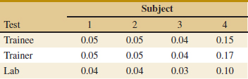
![]()
13-50. An article in the Food Technology Journal (1956, Vol. 10, pp. 39–42) described a study on the protopectin content of tomatoes during storage. Four storage times were selected, and samples from nine lots of tomatoes were analyzed. The protopectin content (expressed as hydrochloric acid soluble fraction mg/kg) is in Table 13E-1.
(a) The researchers in this study hypothesized that mean protopectin content would be different at different storage times. Can you confirm this hypothesis with a statistical test using α = 0.05?
(b) Find the P-value for the test in part (a).
(c) Which specific storage times are different? Would you agree with the statement that protopectin content decreases as storage time increases?
(d) Analyze the residuals from this experiment.
![]()
13-51. An experiment was conducted to investigate leaking current in a SOS MOSFETS device. The purpose of the experiment was to investigate how leakage current varies as the channel length changes. Four channel lengths were selected. For each channel length, five different widths were also used, and width is to be considered a nuisance factor. The data are as follows:
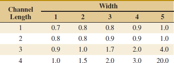
(a) Test the hypothesis that mean leakage voltage does not depend on the channel length using α = 0.05.
(b) Analyze the residuals from this experiment. Comment on the residual plots.
(c) The observed leakage voltage for channel length 4 and width 5 was erroneously recorded. The correct observation is 4.0. Analyze the corrected data from this experiment. Is there evidence to conclude that mean leakage voltage increases with channel length?
![]() TABLE • 13E-1 Protopectin Content of Tomatoes in Storage
TABLE • 13E-1 Protopectin Content of Tomatoes in Storage

![]() Problem available in WileyPLUS at instructor's discretion.
Problem available in WileyPLUS at instructor's discretion.
![]() Go Tutorial Tutoring problem available in WileyPLUS at instructor's discretion.
Go Tutorial Tutoring problem available in WileyPLUS at instructor's discretion.
13-52. Consider the following computer output.
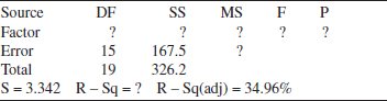
(a) How many levels of the factor were used in this experiment?
(b) How many replicates were used?
(c) Fill in the missing information. Use bounds for the P-value.
(d) What conclusions would you draw if α = 0.05? What if α = 0.01?
13-53. Consider the following computer output.
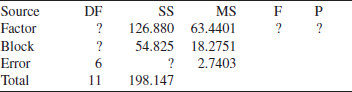
(a) How many levels of the factor were used in this experiment?
(b) How many blocks were used?
(c) Fill in the missing information. Use bounds for the P-value.
(d) What conclusions would you draw if α = 0.05? What if α = 0.01?
![]() 13-54.
13-54. ![]() An article in Lubrication Engineering (December 1990) described the results of an experiment designed to investigate the effects of carbon material properties on the progression of blisters on carbon face seals. The carbon face seals are used extensively in equipment such as air turbine starters. Five different carbon materials were tested, and the surface roughness was measured. The data are as follows:
An article in Lubrication Engineering (December 1990) described the results of an experiment designed to investigate the effects of carbon material properties on the progression of blisters on carbon face seals. The carbon face seals are used extensively in equipment such as air turbine starters. Five different carbon materials were tested, and the surface roughness was measured. The data are as follows:
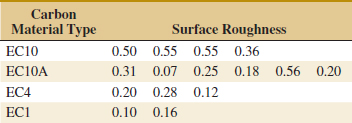
(a) Does carbon material type have an effect on mean surface roughness? Use α = 0.05.
(b) Find the residuals for this experiment. Does a normal probability plot of the residuals indicate any problem with the normality assumption?
(c) Plot the residuals versus ![]() ij. Comment on the plot.
ij. Comment on the plot.
(d) Find a 95% confidence interval on the difference between mean surface roughness for the EC10 and the EC1 carbon grades.
(e) Apply the Fisher LSD method to this experiment. Summarize your conclusions regarding the effect of material type on surface roughness.
![]()
13-55. ![]() An article in the IEEE Transactions on Components, Hybrids, and Manufacturing Technology [(1992, Vol. 15(2), pp. 146–153)] described an experiment in which the contact resistance of a brake-only relay was studied for three different materials (all were silver-based alloys). The data are as follows.
An article in the IEEE Transactions on Components, Hybrids, and Manufacturing Technology [(1992, Vol. 15(2), pp. 146–153)] described an experiment in which the contact resistance of a brake-only relay was studied for three different materials (all were silver-based alloys). The data are as follows.
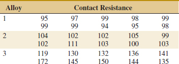
(a) Does the type of alloy affect mean contact resistance? Use α = 0.01.
(b) Use Fisher's LSD method to determine which means differ.
(c) Find a 99% confidence interval on the mean contact resistance for alloy 3.
(d) Analyze the residuals for this experiment.
![]()
13-56. An article in the Journal of Quality Technology [(1982, Vol. 14(2), pp. 80–89)] described an experiment in which three different methods of preparing fish were evaluated on the basis of sensory criteria, and a quality score was assigned. Assume that these methods have been randomly selected from a large population of preparation methods. The data are in the following table:

(a) Is there any difference in preparation methods? Use α = 0.05.
(b) Calculate the P-value for the F-statistic in part (a).
(c) Analyze the residuals from this experiment and comment on model adequacy.
(d) Estimate the components of variance.
![]()
13-57. ![]() An article in the Journal of Agricultural Engineering Research (1992, Vol. 52, pp. 53–76) described an experiment to investigate the effect of drying temperature of wheat grain on baking quality bread. Three temperature levels were used, and the response variable measured was the volume of the loaf of bread produced. The data are as follows:
An article in the Journal of Agricultural Engineering Research (1992, Vol. 52, pp. 53–76) described an experiment to investigate the effect of drying temperature of wheat grain on baking quality bread. Three temperature levels were used, and the response variable measured was the volume of the loaf of bread produced. The data are as follows:
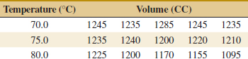
(a) Does drying temperature affect mean bread volume? Use α = 0.01.
(b) Find the P-value for this test.
(c) Use the Fisher LSD method to determine which means are different.
(d) Analyze the residuals from this experiment and comment on model adequacy.
![]() 13-58. An article in Agricultural Engineering (December 1964, pp. 672–673) described an experiment in which the daily weight gain of swine is evaluated at different levels of housing temperature. The mean weight of each group of swine at the start of the experiment is considered to be a nuisance factor. The data from this experiment are as follows:
13-58. An article in Agricultural Engineering (December 1964, pp. 672–673) described an experiment in which the daily weight gain of swine is evaluated at different levels of housing temperature. The mean weight of each group of swine at the start of the experiment is considered to be a nuisance factor. The data from this experiment are as follows:
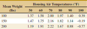
(a) Does housing air temperature affect mean weight gain? Use α = 0.05.
(b) Use Fisher's LSD method to determine which temperature levels are different.
(c) Analyze the residuals from this experiment and comment on model adequacy.
![]() 13-59.
13-59. ![]() An article in Communications of the ACM [(1987, Vol. 30(5), pp. 53–76] reported on a study of different algorithms for estimating software development costs. Six algorithms were applied to eight software development projects and the percent error in estimating the development cost was observed. The data are in Table 13E-2.
An article in Communications of the ACM [(1987, Vol. 30(5), pp. 53–76] reported on a study of different algorithms for estimating software development costs. Six algorithms were applied to eight software development projects and the percent error in estimating the development cost was observed. The data are in Table 13E-2.
(a) Do the algorithms differ in mean cost estimation accuracy? Use α = 0.05.
(b) Analyze the residuals from this experiment.
(c) Which algorithm would you recommend for use in practice?
![]() 13-60. An article in Nature Genetics [(2003, Vol. 34(1), pp. 85–90)], “Treatment-Specific Changes in Gene Expression Discriminate in vivo Drug Response in Human Leukemia Cells,” reported the results of a study of gene expression as a function of different treatments for leukemia. Three treatment groups are mercaptopurine (MP) only, low-dose methotrexate (LDMTX) and MP, and high-dose methotrexate (HDMTX) and MP. Each group contained ten subjects. The responses from a specific gene are shown in Table 13E-3.
13-60. An article in Nature Genetics [(2003, Vol. 34(1), pp. 85–90)], “Treatment-Specific Changes in Gene Expression Discriminate in vivo Drug Response in Human Leukemia Cells,” reported the results of a study of gene expression as a function of different treatments for leukemia. Three treatment groups are mercaptopurine (MP) only, low-dose methotrexate (LDMTX) and MP, and high-dose methotrexate (HDMTX) and MP. Each group contained ten subjects. The responses from a specific gene are shown in Table 13E-3.
(a) Check the normality of the data. Can you assume that these samples are from normal populations?
(b) Take the logarithm of the raw data and check the normality of the transformed data. Is there evidence to support the claim that the treatment means differ for the transformed data? Use α = 0.1.
(c) Analyze the residuals from the transformed data and comment on model adequacy.
13-61. ![]() Consider an ANOVA situation with a = 5 treatments. Let σ2 = 9 and α = 0.05, and suppose that n = 4.
Consider an ANOVA situation with a = 5 treatments. Let σ2 = 9 and α = 0.05, and suppose that n = 4.
(a) Find the power of the ANOVA F-test when μ1 = μ2 = μ3 = 1, μ4 = 3, and μ5 = 2.
(b) What sample size is required if you want the power of the F-test in this situation to be at least 0.90?
13-62. ![]() Consider an ANOVA situation with a = 4 means μ1 = 1, μ2 = 5, μ3 = 8, and μ5 = 4. Suppose that σ2 = 4, n = 4, and α = 0.05.
Consider an ANOVA situation with a = 4 means μ1 = 1, μ2 = 5, μ3 = 8, and μ5 = 4. Suppose that σ2 = 4, n = 4, and α = 0.05.
(a) Find the power of the ANOVA F-test.
(b) How large would the sample size have to be if you want the power of the F-test for detecting this difference in means to be at least 0.90?
13-63. An article in Marine Biology [“Allozymes an Morphometric Characters of Three Species of Mytilus in the Northern and Southern Hemispheres” (1991, Vol. 111, pp. 323–333)] discussed the ratio of the anterior adductor muscle scar length to shell length for shells from five different geographic locations. The following table is part of a much larger data set from their research.

![]() TABLE • 13E-2 Software Development Costs
TABLE • 13E-2 Software Development Costs
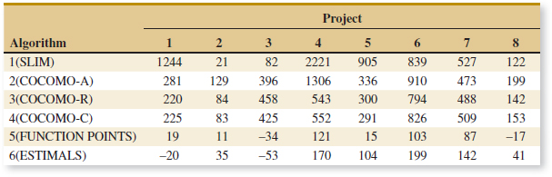
![]() TABLE • 13E-3 Treatment-Specific Changes in Gene Expression
TABLE • 13E-3 Treatment-Specific Changes in Gene Expression

(a) Are there differences in the mean ratios due to different locations at α = 0.05? Calculate the P-value.
(b) Analyze the residuals from the experiment. In particular, comment on the normality assumption.
13-64. An article in Bioresource Technology [“Preliminary Tests on Nisin and Pediocin Production Using Waste Protein Sources: Factorial and Kinetic Studies” (2006, Vol. 97(4), pp. 605–613)] described an experiment in which pediocin was produced from waste protein. Nisin and pediocin are bacteriocins (compounds produced by bacteria that inhibit related strains) used for food preservation. Three levels of protein (g/L) from trout viscera extracts were compared.

(a) Construct box plots of the data. What visual impression do you have from these plots?
(b) Does the level of protein have an effect on mean pediocin production? Use α = 0.05.
(c) Would you draw a different conclusion if α = 0.01 had been used?
(d) Plot the residuals from the experiment and comment. In particular, comment on the normality of the residuals.
(e) Find a 95% confidence interval on mean pediocin production when the level of protein is 2.50 g/L.
13-65. Reconsider Exercise 13-9 in which the effect of different coating types on conductivity was investigated. Suppose that the five coating types were selected at random from a large number of types.
(a) How does this change the interpretation of the experiment?
(b) What is an appropriate statistical model for this experiment?
(c) Estimate the parameters of this model.
13-66. An article in Journal of Hazardous Materials [“Toxicity Assessment from Electro-Coagulation Treated-Textile Dye Waste Waters by Bioassays,” 2009, Vol. 172(1), pp. 330–337] discussed a study of pollutant removal from textile dyeing waste water with an electro-coagulation technique. Chemical oxygen demand (COD) (a common measure of water pollution) was used as the response, and three different values for electrolysis time were considered. The following data were extracted from a larger study. Suppose that a randomized complete block experiment was conducted with three blocks based on initial pH values.

(a) Is there an effect of electrolysis time at α = 0.05? Calculate the P-value.
(b) Analyze the residuals from the experiment.
(c) Calculate a 95% confidence interval on mean COD removal when the electrolysis time is 15 minutes.
(d) Perform an ANOVA assuming that all data are collected at a single pH value. Comment on differences from part (a).
Mind-Expanding Exercises
13-67. Show that in the fixed-effects model analysis of variance E(MSE) = σ2. How would your development change if the random-effects model had been specified?
13-68. Consider testing the equality of the means of two normal populations for which the variances are unknown but are assumed to be equal. The appropriate test procedure is the two-sample t-test. Show that the two-sample t-test is equivalent to the single-factor analysis of variance F-test.
13-69. Consider the ANOVA with a = 2 treatments. Show that the MSE in this analysis is equal to the pooled variance estimate used in the two-sample t-test.
13-70. Show that the variance of the linear combination
![]()
13-71. In a fixed-effects model, suppose that there are n observations for each of four treatments. Let ![]() , and
, and ![]() be single-degree-of-freedom sums of squares for orthogonal contrasts. A contrast is a linear combination of the treatment means with coefficients that sum to zero. The coefficient vectors of orthogonal contrasts are orthogonal vectors. Prove that SSTreatments =
be single-degree-of-freedom sums of squares for orthogonal contrasts. A contrast is a linear combination of the treatment means with coefficients that sum to zero. The coefficient vectors of orthogonal contrasts are orthogonal vectors. Prove that SSTreatments = ![]() .
.
13-72. Consider the single-factor completely randomized design with a treatments and n replicates. Show that if the difference between any two treatment means is as large as D, the minimum value that the OC curve parameter Φ2 can take is
![]()
13-73. Consider the single-factor completely randomized design. Show that a 100(1 − α) percent confidence interval for σ2 is
![]()
where N is the total number of observations in the experimental design.
13-74. Consider the random-effects model for the single-factor completely randomized design. Show that a 100(1 − α)% confidence interval on the ratio of variance components ![]() is given by
is given by
![]()
where
![]()
and
![]()
13-75. Consider a random-effects model for the single-factor completely randomized design.
(a) Show that a 100(1 − α)% confidence interval on the ratio ![]() is
is
![]()
where L and U are as defined in Exercise 13-74.
(b) Use the results of part (a) to find a 100(1 − α)% confidence interval for σ2/(σ2 + ![]() ).
).
13-76. Consider the fixed-effects model of the completely randomized single-factor design. The model parameters are restricted by the constraint ![]() . (Actually, other restrictions could be used, but this one is simple and results in intuitively pleasing estimates for the model parameters.) For the case of unequal sample size n1, n2,..., na, the restriction is
. (Actually, other restrictions could be used, but this one is simple and results in intuitively pleasing estimates for the model parameters.) For the case of unequal sample size n1, n2,..., na, the restriction is ![]() . Use this to show that
. Use this to show that
![]()
Does this suggest that the null hypothesis in this model is H0: n1τ1 = n1τ2 = ··· = naτa = 0?
13-77. Sample Size Determination. In the single-factor completely randomized design, the accuracy of a 100(1 − α)% confidence interval on the difference in any two treatment means is tα/2,a(n−1)![]() .
.
(a) Show that if A is the desired accuracy of the interval, the sample size required is
![]()
(b) Suppose that in comparing a = 5 means you have a preliminary estimate of σ2 of 4. If you want the 95% confidence interval on the difference in means to have an accuracy of 2, how many replicates should you use?
Important Terms and Concepts
Analysis of variance (ANOVA)
Blocking
Completely randomized design (CRD)
Error mean square
Fisher's least significant difference (LSD) method
Fixed-effects model
Graphical comparison of means
Least significant difference
Levels of a factor
Linear statistical model
Mean squares
Multiple comparisons methods
Nuisance factor
Operating characteristic curve
Random factor-effects model
Randomization
Randomized complete block design (RCBD)
Replicates
Residual analysis and model checking
Sample size and replication in an experiment
Treatment
Treatment sum of squares
Variance component
*The assumption that the {τi} are independent random variables implies that the usual assumption of ![]() = 0 from the fixed-effects model does not apply to the random-effects model.
= 0 from the fixed-effects model does not apply to the random-effects model.