

Multiple Linear Regression

Chapter Outline
12-1 Multiple Linear Regression Model
12-1.2 Least Squares Estimation of the Parameters
12-1.3 Matrix Approach to Multiple Linear Regression
12-1.4 Properties of the Least Squares Estimators
12-2 Hypothesis Tests in Multiple Linear Regression
12-2.1 Test for Significance of Regression
12-2.2 Tests on Individual Regression Coefficients and Subsets of Coefficients
12-3 Confidence Intervals in Multiple Linear Regression
12-3.1 Confidence Intervals on Individual Regression Coefficients
12-3.2 Confidence Interval on the Mean Response
12-4 Prediction of New Observations
12-5.2 Influential Observations
12-6 Aspects of Multiple Regression Modeling
12-6.1 Polynomial Regression Models
12-6.2 Categorical Regressors and Indicator Variables
This chapter generalizes the simple linear regression to a situation that has more than one predictor or regressor variable. This situation occurs frequently in science and engineering; for example, in Chapter 1, we provided data on the pull strength of a wire bond on a semiconductor package and illustrated its relationship to the wire length and the die height. Understanding the relationship between strength and the other two variables may provide important insight to the engineer when the package is designed, or to the manufacturing personnel who assemble the die into the package. We used a multiple linear regression model to relate strength to wire length and die height. There are many examples of such relationships: The life of a cutting tool is related to the cutting speed and the tool angle; patient satisfaction in a hospital is related to patient age, type of procedure performed, and length of stay; and the fuel economy of a vehicle is related to the type of vehicle (car versus truck), engine displacement, horsepower, type of transmission, and vehicle weight. Multiple regression models give insight into the relationships between these variables that can have important practical implications.
In this chapter, we show how to fit multiple linear regression models, perform the statistical tests and confidence procedures that are analogous to those for simple linear regression, and check for model adequacy. We also show how models that have polynomial terms in the regressor variables are just multiple linear regression models. We also discuss some aspects of building a good regression model from a collection of candidate regressors.
![]() Learning Objectives
Learning Objectives
After careful study of this chapter, you should be able to do the following:
- Use multiple regression techniques to build empirical models to engineering and scientific data
- Understand how the method of least squares extends to fitting multiple regression models
- Assess regression model adequacy
- Test hypotheses and construct confidence intervals on the regression coefficients
- Use the regression model to estimate the mean response and to make predictions and to construct confidence intervals and prediction intervals
- Build regression models with polynomial terms
- Use indicator variables to model categorical regressors
- Use stepwise regression and other model building techniques to select the appropriate set of variables for a regression model
12-1 Multiple Linear Regression Model
12-1.1 INTRODUCTION
Many applications of regression analysis involve situations that have more than one regressor or predictor variable. A regression model that contains more than one regressor variable is called a multiple regression model.
As an example, suppose that the gasoline mileage performance of a vehicle depends on the vehicle weight and the engine displacement. A multiple regression model that might describe this relationship is
![]()
where Y represents the mileage, x1 represents the weight, x2 represents the engine displacement, and ![]() is a random error term. This is a multiple linear regression model with two regressors. The term linear is used because Equation 12-1 is a linear function of the unknown parameters β0, β1, and β2.
is a random error term. This is a multiple linear regression model with two regressors. The term linear is used because Equation 12-1 is a linear function of the unknown parameters β0, β1, and β2.
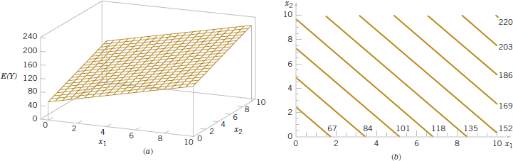
FIGURE 12-1 (a) The regression plane for the model E(Y) = 50 + 10x1 + 7x2. (b) The contour plot.
The regression model in Equation 12-1 describes a plane in the three-dimensional space of Y, x1, and x2. Figure 12-1(a) shows this plane for the regression model
![]()
where we have assumed that the expected value of the error term is zero; that is E(![]() ) = 0. The parameter β0 is the intercept of the plane. We sometimes call β1 and β2 partial regression coefficients because β1 measures the expected change in Y per unit change in x1 when x2 is held constant, and β2 measures the expected change in Y per unit change in x2 when x1 is held constant. Figure 12-1(b) shows a contour plot of the regression model—that is, lines of constant E(Y) as a function of x1 and x2. Notice that the contour lines in this plot are straight lines.
) = 0. The parameter β0 is the intercept of the plane. We sometimes call β1 and β2 partial regression coefficients because β1 measures the expected change in Y per unit change in x1 when x2 is held constant, and β2 measures the expected change in Y per unit change in x2 when x1 is held constant. Figure 12-1(b) shows a contour plot of the regression model—that is, lines of constant E(Y) as a function of x1 and x2. Notice that the contour lines in this plot are straight lines.
In general, the dependent variable or response Y may be related to k independent or regressor variables. The model
![]()
is called a multiple linear regression model with k regressor variables. The parameters βj, j = 0,1,..., k, are called the regression coefficients. This model describes a hyperplane in the k-dimensional space of the regressor variables {xj}. The parameter βj represents the expected change in response Y per unit change in xj when all the remaining regressors xi(i ≠ j) are held constant.
Multiple linear regression models are often used as approximating functions. That is, the true functional relationship between Y and x1, x2,..., xk is unknown, but over certain ranges of the independent variables, the linear regression model is an adequate approximation.
Models that are more complex in structure than Equation 12-2 may often still be analyzed by multiple linear regression techniques. For example, consider the cubic polynomial model in one regressor variable.
![]()
If we let x1 = x, x2 = x2, x3 = x3, Equation 12-3 can be written as
![]()
which is a multiple linear regression model with three regressor variables.
Models that include interaction effects may also be analyzed by multiple linear regression methods. Interaction effects are very common. For example, a vehicle's mileage may be impacted by an interaction between vehicle weight and engine displacement. An interaction between two variables can be represented by a cross-product term in the model, such as
![]()
If we let x3 = x1x2 and β3 = β12, Equation 12-5 can be written as
![]()
which is a linear regression model.
Figure 12-2(a) and (b) shows the three-dimensional plot of the regression model
![]()
and the corresponding two-dimensional contour plot. Notice that, although this model is a linear regression model, the shape of the surface that is generated by the model is not linear. In general, any regression model that is linear in parameters (the β's) is a linear regression model, regardless of the shape of the surface that it generates.
Figure 12-2 provides a nice graphical interpretation of an interaction. Generally, interaction implies that the effect produced by changing one variable (x1, say) depends on the level of the other variable (x2). For example, Fig. 12-2 shows that changing x1 from 2 to 8 produces a much smaller change in E(Y) when x2 = 2 than when x2 = 10. Interaction effects occur frequently in the study and analysis of real-world systems, and regression methods are one of the techniques that we can use to describe them.
As a final example, consider the second-order model with interaction
![]()
If we let x3 = ![]() , x4 =
, x4 = ![]() , x5 = x1x2, β3 = β11, β4 = β22, and β5 = β12, Equation 12-6 can be written as a multiple linear regression model as follows:
, x5 = x1x2, β3 = β11, β4 = β22, and β5 = β12, Equation 12-6 can be written as a multiple linear regression model as follows:
![]()
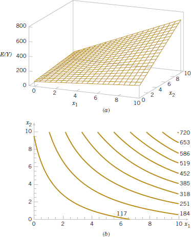
FIGURE 12-2 (a) Three-dimensional plot of the regression model. (b) The contour plot.
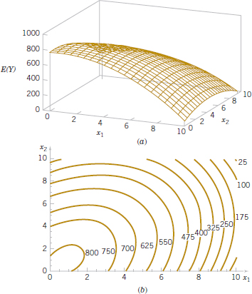
FIGURE 12-3 (a) Three-dimensional plot of the regression model E(Y) = 800 + 10x1 + 7x2 − 8.5![]() − 5
− 5![]() + 4x1x2. (b) The contour plot.
+ 4x1x2. (b) The contour plot.
Figure 12-3 parts (a) and (b) show the three-dimensional plot and the corresponding contour plot for
![]()
These plots indicate that the expected change in Y when xi is changed by one unit (say) is a function of and x2. The quadratic and interaction terms in this model produce a mound-shaped function. Depending on the values of the regression coefficients, the second-order model with interaction is capable of assuming a wide variety of shapes; thus, it is a very flexible regression model.
12-1.2 LEAST SQUARES ESTIMATION OF THE PARAMETERS
The method of least squares may be used to estimate the regression coefficients in the multiple regression model, Equation 12-2. Suppose that n > k observations are available, and let xij denote the ith observation or level of variable xj. The observations are
![]()
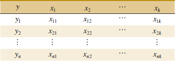
It is customary to present the data for multiple regression in a table such as Table 12-1.
Each observation (xi1, xi2, ..., xik, yi), satisfies the model in Equation 12-2, or
The least squares function is
![]()
We want to minimize L with respect to β0, β1,..., βk. The least squares estimates of β0, β1,..., βk must satisfy
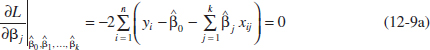
and
![]()
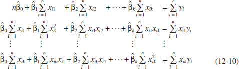
Simplifying Equation 12-9, we obtain the least squares normal equations
![]() TABLE • 12-1 Data for Multiple Linear Regression
TABLE • 12-1 Data for Multiple Linear Regression
Note that there are p = k + 1 normal equations, one for each of the unknown regression coefficients. The solution to the normal equations will be the least squares estimators of the regression coefficients, ![]() 0,
0, ![]() 1,...,
1,...,![]() k. The normal equations can be solved by any method appropriate for solving a system of linear equations.
k. The normal equations can be solved by any method appropriate for solving a system of linear equations.
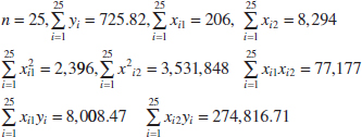
Example 12-1 Wire Bond Strength In Chapter 1, we used data on pull strength of a wire bond in a semiconductor manufacturing process, wire length, and die height to illustrate building an empirical model. We will use the same data, repeated for convenience in Table 12-2, and show the details of estimating the model parameters. A three-dimensional scatter plot of the data is presented in Fig. 1-15. Figure 12-4 is a matrix of two-dimensional scatter plots of the data. These displays can be helpful in visualizing the relationships among variables in a multivariable data set. For example, the plot indicates that there is a strong linear relationship between strength and wire length.
Specifically, we will fit the multiple linear regression model
![]()
where Y = pull strength, x1 = wire length, and x2 = die height. From the data in Table 12-2, we calculate
For the model Y = β0 + β1x1 + β2x2 + ![]() , the normal Equations 12-10 are
, the normal Equations 12-10 are
![]() TABLE • 12-2 Wire Bond Data for Example 12-1
TABLE • 12-2 Wire Bond Data for Example 12-1
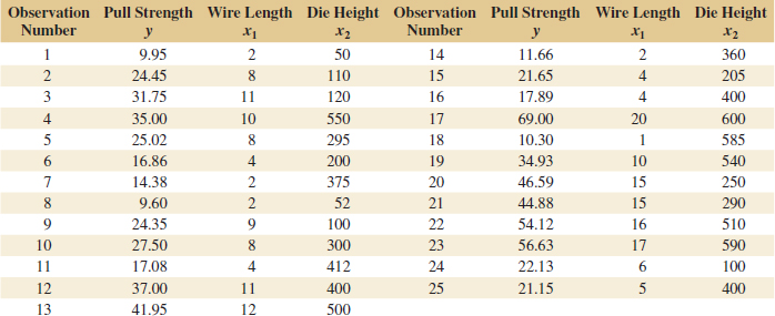

FIGURE 12-4 Matrix of computer-generated scatter plots for the wire bond pull strength data in Table 12-2.
Inserting the computed summations into the normal equations, we obtain

The solution to this set of equations is
![]()
Therefore, the fitted regression equation is
![]()
Practical Interpretation: This equation can be used to predict pull strength for pairs of values of the regressor variables wire length (x1) and die height (x2). This is essentially the same regression model given in Section 1-3. Figure 1-16 shows a three-dimensional plot of the plane of predicted values ![]() generated from this equation.
generated from this equation.
12-1.3 MATRIX APPROACH TO MULTIPLE LINEAR REGRESSION
In fitting a multiple regression model, it is much more convenient to express the mathematical operations using matrix notation. Suppose that there are k regressor varibles and n observations, (xi1, xi2,...,xik, yi), i = 1,2,...,n and that the model relating the regressors to the response is
![]()
This model is a system of n equations that can be expressed in matrix notation as
![]()
where

In general, y is an (n × 1) vector of the observations, X is an (n × p) matrix of the levels of the independent variables (assuming that the intercept is always multiplied by a constant value—unity), β is a (p × 1) vector of the regression coefficients, and ![]() is a (n × 1) vector of random errors. The X matrix is often called the model matrix.
is a (n × 1) vector of random errors. The X matrix is often called the model matrix.
We wish to find the vector of least squares estimators, ![]() , that minimizes
, that minimizes
![]()
The least squares estimator ![]() is the solution for β in the equations
is the solution for β in the equations
![]()
We will not give the details of taking the preceding derivatives; however, the resulting equations that must be solved are
Normal Equations
![]()
Equations 12-12 are the least squares normal equations in matrix form. They are identical to the scalar form of the normal equations given earlier in Equations 12-10. To solve the normal equations, multiply both sides of Equations 12-12 by the inverse of X′X. Therefore, the least squares estimate of β is
Least Squares Estimate of β
![]()
Note that there are p = k + 1 normal equations in p = k + 1 unknowns (the values of ![]() 0,
0, ![]() 1,...,
1,..., ![]() k). Furthermore, the matrix X′X is always nonsingular, as was assumed previously, so the methods described in textbooks on determinants and matrices for inverting these matrices can be used to find (X′X)−1. In practice, multiple regression calculations are almost always performed using a computer.
k). Furthermore, the matrix X′X is always nonsingular, as was assumed previously, so the methods described in textbooks on determinants and matrices for inverting these matrices can be used to find (X′X)−1. In practice, multiple regression calculations are almost always performed using a computer.
It is easy to see that the matrix form of the normal equations is identical to the scalar form. Writing out Equation 12-12 in detail, we obtain
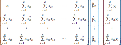
If the indicated matrix multiplication is performed, the scalar form of the normal equations (that is, Equation 12-10) will result. In this form, it is easy to see that X′X is a (p × p) symmetric matrix and X′y is a (p × 1) column vector. Note the special structure of the X′X matrix. The diagonal elements of X′X are the sums of squares of the elements in the columns of X, and the off-diagonal elements are the sums of cross-products of the elements in the columns of X. Furthermore, note that the elements of X′y are the sums of cross-products of the columns of X and the observations {yi}.
The fitted regression model is
![]()
In matrix notation, the fitted model is
![]()
The difference between the observation yi and the fitted value ![]() i is a residual, say, ei = yi −
i is a residual, say, ei = yi − ![]() i.
i.
The (n × 1) vector of residuals is denoted by
![]()
Example 12-2 Wire Bond Strength With Matrix Notation In Example 12-1, we illustrated fitting the multiple regression model
![]()
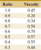
where y is the observed pull strength for a wire bond, x1 is the wire length, and x2 is the die height. The 25 observations are in Table 12-2. We will now use the matrix approach to fit the previous regression model to these data. The model matrix X and y vector for this model are
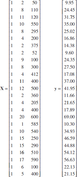

and the X′y vector is
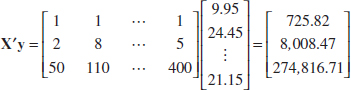
The least squares estimates are found from Equation 12-13 as
![]()
or
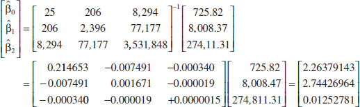
Therefore, the fitted regression model with the regression coefficients rounded to five decimal places is
![]()
This is identical to the results obtained in Example 12-1.
This regression model can be used to predict values of pull strength for various values of wire length (x1) and die height (x2). We can also obtain the fitted values ![]() i by substituting each observation (xi1, xi2), i = 1,2,..., n, into the equation. For example, the first observation has x11 = 2 and x12 = 50, and the fitted value is
i by substituting each observation (xi1, xi2), i = 1,2,..., n, into the equation. For example, the first observation has x11 = 2 and x12 = 50, and the fitted value is
![]()
![]() TABLE • 12-3 Observations, Fitted Values, and Residuals for Example 12-2
TABLE • 12-3 Observations, Fitted Values, and Residuals for Example 12-2
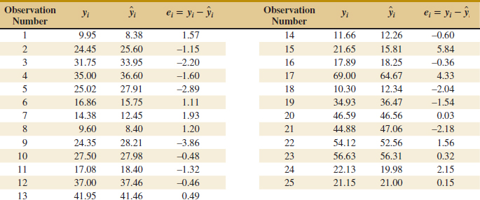
The corresponding observed value is y1 = 9.95. The residual corresponding to the first observation is
![]()
Table 12-3 displays all 25 fitted values ![]() i and the corresponding residuals. The fitted values and residuals are calculated to the same accuracy as the original data.
i and the corresponding residuals. The fitted values and residuals are calculated to the same accuracy as the original data.
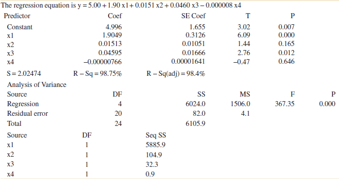
Computers are almost always used in fitting multiple regression models. See Table 12-4 for some annotated computer output for the least squares regression model for the wire bond pull strength data. The upper part of the table contains the numerical estimates of the regression coefficients. The computer also calculates several other quantities that reflect important information about the regression model. In subsequent sections, we will define and explain the quantities in this output.
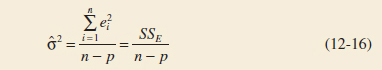
Estimating σ2
Just as in simple linear regression, it is important to estimate σ2, the variance of the error term ![]() , in a multiple regression model. Recall that in simple linear regression the estimate of σ2 was obtained by dividing the sum of the squared residuals by n − 2. Now there are two parameters in the simple linear regression model, so in multiple linear regression with p parameters, a logical estimator for σ2 is
, in a multiple regression model. Recall that in simple linear regression the estimate of σ2 was obtained by dividing the sum of the squared residuals by n − 2. Now there are two parameters in the simple linear regression model, so in multiple linear regression with p parameters, a logical estimator for σ2 is
Estimator of Variance
![]() TABLE • 12-4 Multiple Regression Output from Software for the Wire Bond Pull Strength Data
TABLE • 12-4 Multiple Regression Output from Software for the Wire Bond Pull Strength Data

This is an unbiased estimator of σ2. Just as in simple linear regression, the estimate of σ2 is usually obtained from the analysis of variance for the regression model. The numerator of Equation 12-16 is called the error or residual sum of squares, and the denominator n − p is called the error or residual degrees of freedom.
We can find a computing formula for SSE as follows:
![]()
Substituting e = y−![]() = y − X
= y − X![]() into the equation, we obtain
into the equation, we obtain
![]()
Table 12-4 shows that the estimate of σ2 for the wire bond pull strength regression model is ![]() 2 = 115.2/22 = 5.2364. The computer output rounds the estimate to
2 = 115.2/22 = 5.2364. The computer output rounds the estimate to ![]() 2 = 5.2.
2 = 5.2.
12-1.4 PROPERTIES OF THE LEAST SQUARES ESTIMATORS
The statistical properties of the least squares estimators ![]() 0,
0, ![]() 1,...,
1,..., ![]() k may be easily found under certain assumptions on the error terms ε1, ε2,..., εn, in the regression model. Paralleling the assumptions made in Chapter 11, we assume that the errors εi are statistically independent with mean zero and variance σ2. Under these assumptions, the least squares estimators
k may be easily found under certain assumptions on the error terms ε1, ε2,..., εn, in the regression model. Paralleling the assumptions made in Chapter 11, we assume that the errors εi are statistically independent with mean zero and variance σ2. Under these assumptions, the least squares estimators ![]() 0,
0, ![]() 1,...,
1,..., ![]() k are unbiased estimators of the regression coefficients β0, β1,..., βk. This property may be shown as follows:
k are unbiased estimators of the regression coefficients β0, β1,..., βk. This property may be shown as follows:
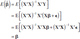
because E(![]() ) = 0 and (X′X)−1 X′X = I, the identity matrix. Thus,
) = 0 and (X′X)−1 X′X = I, the identity matrix. Thus, ![]() is an unbiased estimator of β.
is an unbiased estimator of β.
The variances of the ![]() 's are expressed in terms of the elements of the inverse of the X′X matrix. The inverse of X′X times the constant σ2 represents the covariance matrix of the regression coefficients
's are expressed in terms of the elements of the inverse of the X′X matrix. The inverse of X′X times the constant σ2 represents the covariance matrix of the regression coefficients ![]() . The diagonal elements of σ2 (X′X)−1 are the variances of
. The diagonal elements of σ2 (X′X)−1 are the variances of ![]() 0,
0, ![]() 1,...,
1,..., ![]() k, and the off-diagonal elements of this matrix are the covariances. For example, if we have k = 2 regressors, such as in the pull strength problem,
k, and the off-diagonal elements of this matrix are the covariances. For example, if we have k = 2 regressors, such as in the pull strength problem,

which is symmetric (C10 = C01, C20 = C02, and C21 = C12) because (X′X)−1 is symmetric, and we have

In general, the covariance matrix of ![]() is a (p × p) symmetric matrix whose jjth element is the variance of
is a (p × p) symmetric matrix whose jjth element is the variance of ![]() j and whose i, jth element is the covariance between
j and whose i, jth element is the covariance between ![]() i and
i and ![]() j, that is,
j, that is,
![]()
The estimates of the variances of these regression coefficients are obtained by replacing σ2 with an estimate. When σ2 is replaced by its estimate ![]() 2, the square root of the estimated variance of the jth regression coefficient is called the estimated standard error of
2, the square root of the estimated variance of the jth regression coefficient is called the estimated standard error of ![]() j or se(
j or se(![]() j) =
j) = ![]() . These standard errors are a useful measure of the precision of estimation for the regression coefficients; small standard errors imply good precision.
. These standard errors are a useful measure of the precision of estimation for the regression coefficients; small standard errors imply good precision.
Multiple regression computer programs usually display these standard errors. For example, the computer output in Table 12-4 reports se(![]() 0) = 1.060, se(
0) = 1.060, se(![]() 1) = 0.09352, and se(
1) = 0.09352, and se(![]() 2) = 0.002798. The intercept estimate is about twice the magnitude of its standard error, and
2) = 0.002798. The intercept estimate is about twice the magnitude of its standard error, and ![]() 1 and β are considerably larger than se(
1 and β are considerably larger than se(![]() 1) and se(
1) and se(![]() 2). This implies reasonable precision of estimation, although the parameters β1 and β2 are much more precisely estimated than the intercept (this is not unusual in multiple regression).
2). This implies reasonable precision of estimation, although the parameters β1 and β2 are much more precisely estimated than the intercept (this is not unusual in multiple regression).
Exercises FOR SECTION 12-1
![]() Problem available in WileyPLUS at instructor's discretion.
Problem available in WileyPLUS at instructor's discretion.
![]() Go Tutorial Tutoring problem available in WileyPLUS at instructor's discretion.
Go Tutorial Tutoring problem available in WileyPLUS at instructor's discretion.
12.1. Exercise 11.1 described a regression model between percent of body fat (%BF) as measured by immersion and BMI from a study on 250 male subjects. The researchers also measured 13 physical characteristics of each man, including his age (yrs), height (in), and waist size (in).
A regression of percent of body fat with both height and waist as predictors shows the following computer output:

(a) Write out the regression model if

and
(b) Verify that the model found from technology is correct to at least 2 decimal places.
(c) What is the predicted body fat of a man who is 6-ft tall with a 34-in waist?
12.2. ![]() A class of 63 students has two hourly exams and a final exam. How well do the two hourly exams predict performance on the final?
A class of 63 students has two hourly exams and a final exam. How well do the two hourly exams predict performance on the final?
The following are some quantities of interest:

(a) Calculate the least squares estimates of the slopes for hourly 1 and hourly 2 and the intercept.
(b) Use the equation of the fitted line to predict the final exam score for a student who scored 70 on hourly 1 and 85 on hourly 2.
(c) If a student who scores 80 on hourly 1 and 90 on hourly 2 gets an 85 on the final, what is her residual?
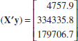
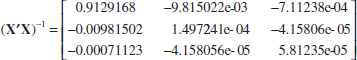
12.3. Can the percentage of the workforce who are engineers in each U.S. state be predicted by the amount of money spent in on higher education (as a percent of gross domestic product), on venture capital (dollars per $1000 of gross domestic product) for high-tech business ideas, and state funding (in dollars per student) for major research universities? Data for all 50 states and a software package revealed the following results:
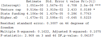
(a) Write the equation predicting the percent of engineers in the workforce.
(b) For a state that has $1 per $1000 in venture capital, spends $10,000 per student on funding for major research universities, and spends 0.5% of its GDP on higher education, what percent of engineers do you expect to see in the workforce?
(c) If the state in part (b) actually had 1.5% engineers in the workforce, what would the residual be?
![]() 12-4. Hsuie, Ma, and Tsai (“Separation and Characterizations of Thermotropic Copolyesters of p-Hydroxybenzoic Acid, Sebacic Acid, and Hydroquinone,” (1995, Vol. 56) studied the effect of the molar ratio of sebacic acid (the regressor) on the intrinsic viscosity of copolyesters (the response). The following display presents the data.
12-4. Hsuie, Ma, and Tsai (“Separation and Characterizations of Thermotropic Copolyesters of p-Hydroxybenzoic Acid, Sebacic Acid, and Hydroquinone,” (1995, Vol. 56) studied the effect of the molar ratio of sebacic acid (the regressor) on the intrinsic viscosity of copolyesters (the response). The following display presents the data.
(a) Construct a scatterplot of the data.
(b) Fit a second-order prediction equation.
12-5. A study was performed to investigate the shear strength of soil (y) as it related to depth in feet (x1) and percent of moisture content (x2). Ten observations were collected, and the following summary quantities obtained: n = 10, Σxi1 = 223, Σxi2 = 553, Σyi = 1,916, ![]() = 5,200.9,
= 5,200.9, ![]() = 31,729, Σxi1xi2 = 12,352, Σxi1yi = 43,550.8, Σxi2yi = 104,736.8, and
= 31,729, Σxi1xi2 = 12,352, Σxi1yi = 43,550.8, Σxi2yi = 104,736.8, and ![]() = 371,595.6.
= 371,595.6.
(a) Set up the least squares normal equations for the model Y = β0 + β1x1 + β2x2 + ![]() .
.
(b) Estimate the parameters in the model in part (a).
(c) What is the predicted strength when x1 = 18 feet and x2 = 43%?
12-6. ![]() A regression model is to be developed for predicting the ability of soil to absorb chemical contaminants. Ten observations have been taken on a soil absorption index (y) and two regressors: x1 = amount of extractable iron ore and x2 = amount of bauxite. We wish to fit the model y = β0 + β1x1 + β2x2 +
A regression model is to be developed for predicting the ability of soil to absorb chemical contaminants. Ten observations have been taken on a soil absorption index (y) and two regressors: x1 = amount of extractable iron ore and x2 = amount of bauxite. We wish to fit the model y = β0 + β1x1 + β2x2 + ![]() .
.
Some necessary quantities are:
(a) Estimate the regression coefficients in the model specified.
(b) What is the predicted value of the absorption index y when x1 = 200 and x2 = 50?
12-7. A chemical engineer is investigating how the amount of conversion of a product from a raw material (y) depends on reaction temperature (x1) and the reaction time (x2). He has developed the following regression models:
 = 100 + 2x1 + 4x2
- = 95 + 1.5x1 + 3x2 + 2x1x2
Both models have been built over the range 0.5 ≤ x2 ≤ 10.
(a) What is the predicted value of conversion when x2 = 2? Repeat this calculation for x2 = 8. Draw a graph of the predicted values for both conversion models. Comment on the effect of the interaction term in model 2.
(b) Find the expected change in the mean conversion for a unit change in temperature x1 for model 1 when x2 = 5. Does this quantity depend on the specific value of reaction time selected? Why?
(c) Find the expected change in the mean conversion for a unit change in temperature x1 for model 2 when x2 = 5. Repeat this calculation for x2 = 2 and x2 = 8. Does the result depend on the value selected for x2? Why?
12-8. You have fit a multiple linear regression model and the (X′X)−1 matrix is:

(a) How many regressor variables are in this model?
(b) If the error sum of squares is 307 and there are 15 observations, what is the estimate of σ2?
(c) What is the standard error of the regression coefficient ![]() 1?
1?
![]()
12-9. The data from a patient satisfaction survey in a hospital are in Table E12-1.
![]() TABLE • E12-1 Patient Satisfaction Data
TABLE • E12-1 Patient Satisfaction Data
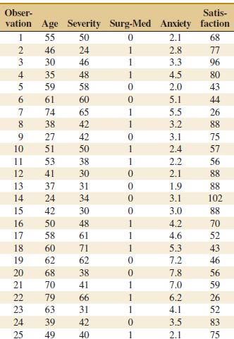
The regressor variables are the patient's age, an illness severity index (higher values indicate greater severity), an indicator variable denoting whether the patient is a medical patient (0) or a surgical patient (1), and an anxiety index (higher values indicate greater anxiety).
(a) Fit a multiple linear regression model to the satisfaction response using age, illness severity, and the anxiety index as the regressors.
(b) Estimate σ2.
(c) Find the standard errors of the regression coefficients.
(d) Are all of the model parameters estimated with nearly the same precision? Why or why not?
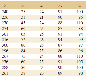
12-10. The electric power consumed each month by a chemical plant is thought to be related to the average ambient temperature (x1), the number of days in the month (x2), the average product purity (x3), and the tons of product produced (x4). The past year's historical data are available and are presented in Table E12-2.
(a) Fit a multiple linear regression model to these data.
(b) Estimate σ2.
(c) Compute the standard errors of the regression coefficients. Are all of the model parameters estimated with the same precision? Why or why not?
(d) Predict power consumption for a month in which x1 = 75°F, x2 = 24 days, x3 = 90%, and x4 = 98 tons.
![]() TABLE • E12-2 Power Consumption Data
TABLE • E12-2 Power Consumption Data
![]()
12-11. Table E12-3 provides the highway gasoline mileage test results for 2005 model year vehicles from DaimlerChrysler. The full table of data (available on the book's Web site) contains the same data for 2005 models from over 250 vehicles from many manufacturers (Environmental Protection Agency Web site www.epa.gov/otaq/cert/mpg/testcars/database).
![]() TABLE • E12-3 DaimlerChrysler Fuel Economy and Emissions
TABLE • E12-3 DaimlerChrysler Fuel Economy and Emissions
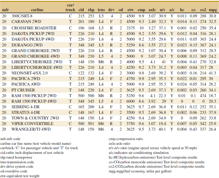
(a) Fit a multiple linear regression model to these data to estimate gasoline mileage that uses the following regressors:
cid, rhp, etw, cmp, axle, n/v
(b) Estimate σ2 and the standard errors of the regression coefficients.
(c) Predict the gasoline mileage for the first vehicle in the table.
12-12. ![]() The pull strength of a wire bond is an important characteristic. Table E12-4 gives information on pull strength (y), die height (x1), post height (x2), loop height (x3), wire length (x4), bond width on the die (x5), and bond width on the post (x6).
The pull strength of a wire bond is an important characteristic. Table E12-4 gives information on pull strength (y), die height (x1), post height (x2), loop height (x3), wire length (x4), bond width on the die (x5), and bond width on the post (x6).
(a) Fit a multiple linear regression model using x2, x3, x4, and x5 as the regressors
(b) Estimate σ2.
(c) Find the se(![]() j). How precisely are the regression coefficients estimated in your opinion?
j). How precisely are the regression coefficients estimated in your opinion?
(d) Use the model from part (a) to predict pull strength when x2 = 20, x3 = 30, x4 = 90, and x5 = 2.0.
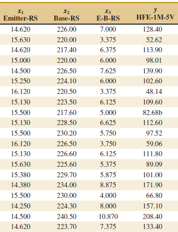
12-13. An engineer at a semiconductor company wants to model the relationship between the device HFE (y) and three parameters: Emitter-RS (x1), Base-RS (x2), and Emitter-to-Base RS (x3). The data are shown in the Table E12-5.
(a) Fit a multiple linear regression model to the data.
(b) Estimate σ2.
(c) Find the standard errors se(![]() j). Are all of the model parameters estimated with the same precision? Justify your answer.
j). Are all of the model parameters estimated with the same precision? Justify your answer.
(d) Predict HFE when x1 = 14.5, x2 = 220, and x3 = 5.0.
![]() TABLE • E12-5 Semiconductor Data
TABLE • E12-5 Semiconductor Data
![]()
12-14. Heat treating is often used to carburize metal parts such as gears. The thickness of the carburized layer is considered a crucial feature of the gear and contributes to the overall reliability of the part. Because of the critical nature of this feature, two different lab tests are performed on each furnace load. One test is run on a sample pin that accompanies each load. The other test is a destructive test that cross-sections an actual part. This test involves running a carbon analysis on the surface of both the gear pitch (top of the gear tooth) and the gear root (between the gear teeth). Table E12-6 shows the results of the pitch carbon analysis test for 32 parts.
![]() TABLE • E12-6 Heat Treating Test
TABLE • E12-6 Heat Treating Test
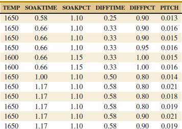
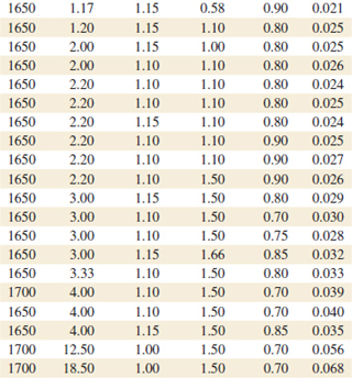
The regressors are furnace temperature (TEMP), carbon concentration and duration of the carburizing cycle (SOAKPCT, SOAKTIME), and carbon concentration and duration of the diffuse cycle (DIFFPCT, DIFFTIME).
(a) Fit a linear regression model relating the results of the pitch carbon analysis test (PITCH) to the five regressor variables.
(b) Estimate σ2.
(c) Find the standard errors se(![]() j)
j)
(d) Use the model in part (a) to predict PITCH when TEMP = 1650, SOAKTIME = 1.00, SOAKPCT = 1.10, DIFFTIME = 1.00, and DIFFPCT = 0.80.
12-15. An article in Electronic Packaging and Production (2002, Vol. 42) considered the effect of X-ray inspection of integrated circuits. The rads (radiation dose) were studied as a function of current (in milliamps) and exposure time (in minutes). The data are in Table E12-7.
![]()
![]() TABLE • E12-7 X-ray Inspection Data
TABLE • E12-7 X-ray Inspection Data
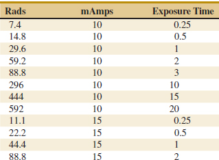
(a) Fit a multiple linear regression model to these data with rads as the response.
(b) Estimate σ2 and the standard errors of the regression coefficients.
(c) Use the model to predict rads when the current is 15 milliamps and the exposure time is 5 seconds.
![]()
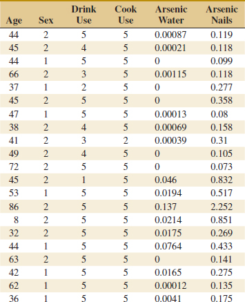
12-16. ![]() An article in Cancer Epidemiology, Biomarkers and Prevention (1996, Vol. 5, pp. 849–852) reported on a pilot study to assess the use of toenail arsenic concentrations as an indicator of ingestion of arsenic-containing water. Twenty-one participants were interviewed regarding use of their private (unregulated) wells for drinking and cooking, and each provided a sample of water and toenail clippings. Table 12-8 showed the data of age (years), sex of person (1 = male, 2 = female), proportion of times household well used for drinking (1 ≤ 1/4,2 = 1/4,3 = 1/2,4 = 3/4,5 ≥ 3/4), proportion of times household well used for cooking (1 ≤ 1/4,2 = 1/4,3 = 1/2,4 = 3/4,5 ≥ 3/4), arsenic in water (ppm), and arsenic in toenails (ppm) respectively.
An article in Cancer Epidemiology, Biomarkers and Prevention (1996, Vol. 5, pp. 849–852) reported on a pilot study to assess the use of toenail arsenic concentrations as an indicator of ingestion of arsenic-containing water. Twenty-one participants were interviewed regarding use of their private (unregulated) wells for drinking and cooking, and each provided a sample of water and toenail clippings. Table 12-8 showed the data of age (years), sex of person (1 = male, 2 = female), proportion of times household well used for drinking (1 ≤ 1/4,2 = 1/4,3 = 1/2,4 = 3/4,5 ≥ 3/4), proportion of times household well used for cooking (1 ≤ 1/4,2 = 1/4,3 = 1/2,4 = 3/4,5 ≥ 3/4), arsenic in water (ppm), and arsenic in toenails (ppm) respectively.
(a) Fit a multiple linear regression model using arsenic concentration in nails as the response and age, drink use, cook use, and arsenic in the water as the regressors.
(b) Estimate σ2 and the standard errors of the regression coefficients.
(c) Use the model to predict the arsenic in nails when the age is 30, the drink use is category 5, the cook use is category 5, and arsenic in the water is 0.135 ppm.
![]() 12-17. An article in IEEE Transactions on Instrumentation and Measurement (2001, Vol. 50, pp. 2033–2040) reported on a study that had analyzed powdered mixtures of coal and limestone for permittivity. The errors in the density measurement was the response. The data are reported in Table E12-9.
12-17. An article in IEEE Transactions on Instrumentation and Measurement (2001, Vol. 50, pp. 2033–2040) reported on a study that had analyzed powdered mixtures of coal and limestone for permittivity. The errors in the density measurement was the response. The data are reported in Table E12-9.

(a) Fit a multiple linear regression model to these data with the density as the response.
(b) Estimate σ2 and the standard errors of the regression coefficients.
(c) Use the model to predict the density when the dielectric constant is 2.5 and the loss factor is 0.03.
![]() 12-18. An article in Biotechnology Progress (2001, Vol. 17, pp. 366–368) reported on an experiment to investigate and optimize nisin extraction in aqueous two-phase systems (ATPS). The nisin recovery was the dependent variable (y). The two regressor variables were concentration (%) of PEG 4000 (denoted as x1 and concentration (%) of Na2SO4 (denoted as x2). The data are in Table E12-10.
12-18. An article in Biotechnology Progress (2001, Vol. 17, pp. 366–368) reported on an experiment to investigate and optimize nisin extraction in aqueous two-phase systems (ATPS). The nisin recovery was the dependent variable (y). The two regressor variables were concentration (%) of PEG 4000 (denoted as x1 and concentration (%) of Na2SO4 (denoted as x2). The data are in Table E12-10.
![]() TABLE • E12-10 Nisin Extraction Data
TABLE • E12-10 Nisin Extraction Data
(a) Fit a multiple linear regression model to these data.
(b) Estimate σ2 and the standard errors of the regression coefficients.
(c) Use the model to predict the nisin recovery when x1 = 14.5 and x2 = 12.5.
![]()
12-19. ![]() An article in Optical Engineering [“Operating Curve Extraction of a Correlator's Filter” (2004, Vol. 43, pp. 2775–2779)] reported on the use of an optical correlator to perform an experiment by varying brightness and contrast. The resulting modulation is characterized by the useful range of gray levels. The data follow:
An article in Optical Engineering [“Operating Curve Extraction of a Correlator's Filter” (2004, Vol. 43, pp. 2775–2779)] reported on the use of an optical correlator to perform an experiment by varying brightness and contrast. The resulting modulation is characterized by the useful range of gray levels. The data follow:
![]()
(a) Fit a multiple linear regression model to these data.
(b) Estimate σ2.
(c) Compute the standard errors of the regression coefficients.
(d) Predict the useful range when brightness = 80 and contrast = 75.
![]()
12-20. An article in Technometrics (1974, Vol. 16, pp. 523–531) considered the following stack-loss data from a plant oxidizing ammonia to nitric acid. Twenty-one daily responses of stack loss (the amount of ammonia escaping) were measured with air flow x1, temperature x2, and acid concentration x3.
(a) Fit a linear regression model relating the results of the stack loss to the three regressor varilables.
(b) Estimate σ2.
(c) Find the standard error se(![]() j).
j).
(d) Use the model in part (a) to predict stack loss when x1 = 60, x2 = 26, and x3 = 85.
![]() 12-21. Table E12-11 presents quarterback ratings for the 2008 National Football League season (The Sports Network).
12-21. Table E12-11 presents quarterback ratings for the 2008 National Football League season (The Sports Network).
(a) Fit a multiple regression model to relate the quarterback rating to the percentage of completions, the percentage of TDs, and the percentage of interceptions.
(b) Estimate σ2.
(c) What are the standard errors of the regression coefficients?
(d) Use the model to predict the rating when the percentage of completions is 60%, the percentage of TDs is 4%, and the percentage of interceptions is 3%.
![]() TABLE • E12-11 Quarterback Ratings for the 2008 National Football League Season
TABLE • E12-11 Quarterback Ratings for the 2008 National Football League Season
![]() 12-22. Table E12-12 presents statistics for the National Hockey League teams from the 2008–2009 season (The Sports Network). Fit a multiple linear regression model that relates wins to the variables GF through FG Because teams play 82 game, W = 82 − L − T − OTL, but such a model does not help build a better team. Estimate σ2 and find the standard errors of the regression coefficients for your model.
12-22. Table E12-12 presents statistics for the National Hockey League teams from the 2008–2009 season (The Sports Network). Fit a multiple linear regression model that relates wins to the variables GF through FG Because teams play 82 game, W = 82 − L − T − OTL, but such a model does not help build a better team. Estimate σ2 and find the standard errors of the regression coefficients for your model.
![]() TABLE • E12-12 Team Statistics for the 2008–2009 National Hockey League Season
TABLE • E12-12 Team Statistics for the 2008–2009 National Hockey League Season

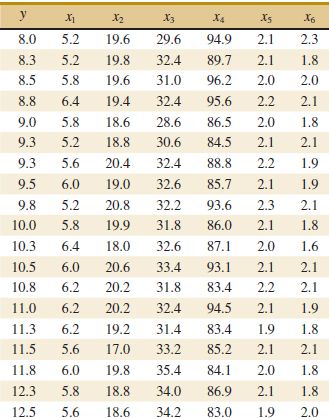
12-23. A study was performed on wear of a bearing and its relationship to x1 = oil viscosity and x2 = load. The following data were obtained.
(a) Fit a multiple linear regression model to these data.
(b) Estimate σ2 and the standard errors of the regression coefficients.
(c) Use the model to predict wear when x1 = 25 and x2 = 1000.
(d) Fit a multiple linear regression model with an interaction term to these data.
(e) Estimate σ2 and se(![]() j) for this new model. How did these quantities change? Does this tell you anything about the value of adding the interaction term to the model?
j) for this new model. How did these quantities change? Does this tell you anything about the value of adding the interaction term to the model?
(f) Use the model in part (d) to predict when x1 = 25 and x2 = 1000. Compare this prediction with the predicted value from part (c).
12-24. Consider the linear regression model
![]()
where ![]() 1 = Σxi1 / n and
1 = Σxi1 / n and ![]() 2 = Σxi2/n.
2 = Σxi2/n.
(a) Write out the least squares normal equations for this model.
(b) Verify that the least squares estimate of the intercept in this model is ![]() 0′ = Σyi / n =
0′ = Σyi / n = ![]() .
.
(c) Suppose that we use yi − ![]() as the response variable in this model. What effect will this have on the least squares estimate of the intercept?
as the response variable in this model. What effect will this have on the least squares estimate of the intercept?
12-2 Hypothesis Tests In Multiple Linear Regression
In multiple linear regression problems, certain tests of hypotheses about the model parameters are useful in measuring model adequacy. In this section, we describe several important hypothesis-testing procedures. As in the simple linear regression case, hypothesis testing requires that the error terms ![]() i in the regression model are normally and independently distributed with mean zero and variance σ2.
i in the regression model are normally and independently distributed with mean zero and variance σ2.
12-2.1 TEST FOR SIGNIFICANCE OF REGRESSION
The test for significance of regression is a test to determine whether a linear relationship exists between the response variable y and a subset of the regressor variables x1, x2,..., xk. The appropriate hypotheses are
Hypotheses for ANOVA Test

Rejection of H0:β1 = β2 = ··· = βk = 0 implies that at least one of the regressor variables x1, x2,..., xk contributes significantly to the model.
The test for significance of regression is a generalization of the procedure used in simple linear regression. The total sum of squares SST is partitioned into a sum of squares due to the model or to regression and a sum of squares due to error, say,
![]()
Now if H0: β1 = β2 = ··· = βk = 0 is true, SSR/σ2 is a chi-square random variable with k degrees of freedom. Note that the number of degrees of freedom for this chi-square random variable is equal to the number of regressor variables in the model. We can also show that the SSE / σ2 is a chi-square random variable with n − p degrees of freedom, and that SSE and SSR are independent. The test statistic for H0: β1 = β2 = ··· = βk = 0 is
![]() TABLE • 12-5 Analysis of Variance for Testing Significance of Regression in Multiple Regression
TABLE • 12-5 Analysis of Variance for Testing Significance of Regression in Multiple Regression

Test Statistic for ANOVA

We should reject H0 if the computed value of the test statistic in Equation 12-19, f0, is greater than fα,k,n−p. The procedure is usually summarized in an analysis of variance table such as Table 12-5.
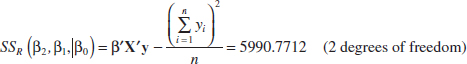
A computational formula for SSR may be found easily. Now because SST = ![]() −
− ![]() /n = y′y −
/n = y′y − ![]() /n, we may rewrite Equation 12-19 as
/n, we may rewrite Equation 12-19 as
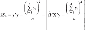
or
![]()
Therefore, the regression sum of squares is
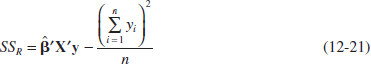
Example 12-3 Wire Bond Strength ANOVA We will test for significance of regression (with α = 0.05) using the wire bond pull strength data from Example 12-1. The total sum of squares is

The regression or model sum of squares is computed from Equation 12-21 as follows:
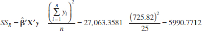
and by subtraction
![]()
The analysis of variance is shown in Table 12-6. To test H0: β1 = β2 = 0, we calculate the statistic
![]()
![]() TABLE • 12-6 Test for Significance of Regression for Example 12-3
TABLE • 12-6 Test for Significance of Regression for Example 12-3
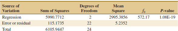
Because f0 > f0.05,2,22 = 3.44 (or because the P-value is considerably smaller than α = 0.05), we reject the null hypothesis and conclude that pull strength is linearly related to either wire length or die height, or both.
Practical Interpretation: Rejection of H0 does not necessarily imply that the relationship found is an appropriate model for predicting pull strength as a function of wire length and die height. Further tests of model adequacy are required before we can be comfortable using this model in practice.
Most multiple regression computer programs provide the test for significance of regression in their output display. The middle portion of Table 12-4 is the computer output for this example. Compare Tables 12-4 and 12-6 and note their equivalence apart from rounding. The P-value is rounded to zero in the computer output.
R2 and Adjusted R2
We may also use the coefficient of multiple determination R2 as a global statistic to assess the fit of the model. Computationally,
![]()
For the wire bond pull strength data, we find that R2 = SSR / SST = 5990.7712 / 6105.9447 = 0.9811. Thus, the model accounts for about 98% of the variability in the pull strength response (refer to the computer software output in Table 12-4). The R2 statistic is somewhat problematic as a measure of the quality of the fit for a multiple regression model because it never decreases when a variable is added to a model.
To illustrate, consider the model fit to the wire bond pull strength data in Example 11-8. This was a simple linear regression model with x1 = wire length as the regressor. The value of R2 for this model is R2 = 0.9640. Therefore, adding x2 = die height to the model increases R2 by 0.9811 − 0.9640 = 0.0171, a very small amount. Because R2 can never decrease when a regressor is added, it can be difficult to judge whether the increase is telling us anything useful about the new regressor. It is particularly hard to interpret a small increase, such as observed in the pull strength data.
Many regression users prefer to use an adjusted R2 statistic:
Adjusted R2

Because SSE /(n − p) is the error or residual mean square and SST /(n − p) is a constant, ![]() will only increase when a variable is added to the model if the new variable reduces the error mean square. Note that for the multiple regression model for the pull strength data
will only increase when a variable is added to the model if the new variable reduces the error mean square. Note that for the multiple regression model for the pull strength data ![]() = 0.979 (see the output in Table 12-4), whereas in Example 11-8, the adjusted R2 for the one-variable model is
= 0.979 (see the output in Table 12-4), whereas in Example 11-8, the adjusted R2 for the one-variable model is ![]() = 0.962. Therefore, we would conclude that adding x2 = die height to the model does result in a meaningful reduction in unexplained variability in the response.
= 0.962. Therefore, we would conclude that adding x2 = die height to the model does result in a meaningful reduction in unexplained variability in the response.
The adjusted R2 statistic essentially penalizes the analyst for adding terms to the model. It is an easy way to guard against overfitting, that is, including regressors that are not really useful. Consequently, it is very useful in comparing and evaluating competing regression models. We will use ![]() for this when we discuss variable selection in regression in Section 12-6.3.
for this when we discuss variable selection in regression in Section 12-6.3.
12-2.2 TESTS ON INDIVIDUAL REGRESSION COEFFICIENTS AND SUBSETS OF COEFFICIENTS
We are frequently interested in testing hypotheses on the individual regression coefficients. Such tests would be useful in determining the potential value of each of the regressor variables in the regression model. For example, the model might be more effective with the inclusion of additional variables or perhaps with the deletion of one or more of the regressors presently in the model.
The hypothesis to test if an individual regression coefficient, say βj equals a value βj0 is
![]()
The test statistic for this hypothesis is
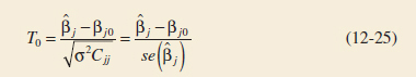
where Cjj is the diagonal element of (X′X)−1 corresponding to ![]() j Notice that the denominator of Equation 12-24 is the standard error of the regression coefficient
j Notice that the denominator of Equation 12-24 is the standard error of the regression coefficient ![]() j. The null hypothesis H0: βj = βj0 is rejected if |t0|>tα/2,n−p. This is called a partial or marginal test because the regression coefficient
j. The null hypothesis H0: βj = βj0 is rejected if |t0|>tα/2,n−p. This is called a partial or marginal test because the regression coefficient ![]() j depends on all the other regressor variables xi(i ≠ j) that are in the model. More will be said about this in the following example.
j depends on all the other regressor variables xi(i ≠ j) that are in the model. More will be said about this in the following example.
An important special case of the previous hypothesis occurs for βj = 0. If H0: βj = 0 is not rejected, this indicates that the regressor xj can be deleted from the model. Adding a variable to a regression model always causes the sum of squares for regression to increase and the error sum of squares to decrease (this is why R2 always increases when a variable is added). We must decide whether the increase in the regression sum of squares is large enough to justify using the additional variable in the model. Furthermore, adding an unimportant variable to the model can actually increase the error mean square, indicating that adding such a variable has actually made the model a poorer fit to the data (this is why ![]() is a better measure of global model fit then the ordinary R2).
is a better measure of global model fit then the ordinary R2).
Example 12-4Wire Bond Strength Coefficient Test Consider the wire bond pull strength data, and suppose that we want to test the hypothesis that the regression coefficient for x2 (die height) is zero. The hypotheses are
![]()
The main diagonal element of the (X′X)−1 matrix corresponding to ![]() 2 is C22 = 0.0000015, so the t-statistic in Equation 12-25 is
2 is C22 = 0.0000015, so the t-statistic in Equation 12-25 is
![]()
Note that we have used the estimate of σ2 reported to four decimal places in Table 12-6. Because t0.025,22 = 2.074, we reject H0: β2 = 0 and conclude that the variable x2 (die height) contributes significantly to the model. We could also have used a P-value to draw conclusions. The P-value for t0 = 4.477 is P = 0.0002, so with α = 0.05, we would reject the null hypothesis.
Practical Interpretation: Note that this test measures the marginal or partial contribution of x2 given that x1 is in the model. That is, the t-test measures the contribution of adding the variable x2 = die height to a model that already contains x1 = wire length. Table 12-4 shows the computer-generated value of the t-test computed. The computer software reports the t-test statistic to two decimal places. Note that the computer produces a t-test for each regression coefficient in the model. These t-tests indicate that both regressors contribute to the model.
Example 12-5 Wire Bond Strength One-Sided Coefficient Test There is an interest in the effect of die height on strength. This can be evaluated by the magnitude of the coefficient for die height. To conclude that the coefficient for die height exceeds 0.01, the hypotheses become
![]()
For such a test, computer software can complete much of the hard work. We need only to assemble the pieces. From the output in Table 12-4, ![]() 2 = 0.012528, and the standard error of
2 = 0.012528, and the standard error of ![]() 2 = 0.002798. Therefore, the t-statistic is
2 = 0.002798. Therefore, the t-statistic is
![]()
with 22 degrees of freedom (error degrees of freedom). From Table IV in Appendix A, t0.25,22 = 0.686 and t0.1,22 = 1.321. Therefore, the P-value can be bounded as 0.1 < P-value < 0.25. One cannot conclude that the coefficient exceeds 0.01 at common levels of significance.
There is another way to test the contribution of an individual regressor variable to the model. This approach determines the increase in the regression sum of squares obtained by adding a variable xj(say) to the model, given that other variables xi(i ≠ j) are already included in the regression equation.
The procedure used to do this is called the general regression significance test, or the extra sum of squares method. This procedure can also be used to investigate the contribution of a subset of the regressor variables to the model. Consider the regression model with k regressor variables
![]()
where y is (n × 1), X is (n × p), β is (p × 1), ![]() is (n × 1), and p = k + 1. We would like to determine whether the subset of regressor variables x1, x2,..., xr(r < k) as a whole contributes significantly to the regression model. Let the vector of regression coefficients be partitioned as follows:
is (n × 1), and p = k + 1. We would like to determine whether the subset of regressor variables x1, x2,..., xr(r < k) as a whole contributes significantly to the regression model. Let the vector of regression coefficients be partitioned as follows:
![]()
where β1 is (r × 1) and β2 is [(p − r) × 1]. We wish to test the hypotheses
Hypotheses for General Regression Test
![]()
where 0 denotes a vector of zeroes. The model may be written as
![]()
where X1 represents the columns of X associated with β1 and X2 represents the columns of X associated with β2.
For the full model (including both β1 and β2), we know that ![]() = (X′X)−1 X′y. In addition, the regression sum of squares for all variables including the intercept is
= (X′X)−1 X′y. In addition, the regression sum of squares for all variables including the intercept is
![]()
and
![]()
SSR(β) is called the regression sum of squares due to β. To find the contribution of the terms in β1 to the regression, fit the model assuming that the null hypothesis H0: β1 = 0 to be true. The reduced model is found from Equation 12-29 as
![]()
The least squares estimate of β2 is β2 = (X2′X2)−1 X2′ y, and
![]()
The regression sum of squares due to β1 given that β2 is already in the model is
![]()
The Extra Sum of Squares
This sum of squares has r degrees of freedom. It is sometimes called the extra sum of squares due to β1. Note that SSR(β1|β2) is the increase in the regression sum of squares due to including the variables x1, x2,..., xr in the model. Now SSR(β1|β2) is independent of MSE, and the null hypothesis β1 = 0 may be tested by the statistic.
F Statistic for General Regression Tests
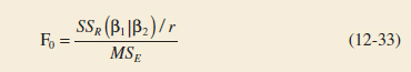
If the computed value of the test statistic f0 > fα,r,n−p, we reject H0, concluding that at least one of the parameters in β1 is not zero and, consequently, at least one of the variables x1, x2,..., xr in X1 contributes significantly to the regression model. Some authors call the test in Equation 12-33 a partial F-test.
The partial F-test is very useful. We can use it to measure the contribution of each individual regressor xj as if it were the last variable added to the model by computing
![]()
This is the increase in the regression sum of squares due to adding xj to a model that already includes x1,...,xj−1, xj+1,...,xk. The partial F-test is a more general procedure in that we can measure the effect of sets of variables. In Section 12-6.3, we show how the partial F-test plays a major role in model building—that is, in searching for the best set of regressor variables to use in the model.
Example 12-6 Wire Bond Strength General Regression Test Consider the wire bond pull-strength data in Example 12-1. We will investigate the contribution of two new variables, x3 and x4, to the model using the partial F-test approach. The new variables are explained at the end of this example. That is, we wish to test
To test this hypothesis, we need the extra sum of squares due to β3 and β4 or
In Example 12-3, we calculated
Also, Table 12-4 shows the computer output for the model with only x1 and x2 as predictors. In the analysis of variance table, we can see that SSR = 5990.8, and this agrees with our calculation. In practice, the computer output would be used to obtain this sum of squares.
If we fit the model Y = β0 + β1x1 + β2x2 + β3x3 + β4x4, we can use the same matrix formula. Alternatively, we can look at SSR from computer output for this model. The analysis of variance table for this model is shown in Table 12-7 and we see that
![]()
Therefore,
![]()
This is the increase in the regression sum of squares due to adding x3 and x4 to a model already containing x1 and x2. To test H0, calculate the test statistic
![]()
Note that MSE from the full model using x1, x2, x3 and x4 is used in the denominator of the test statistic. Because f0.05,2, 20 = 3.49, we reject H0 and conclude that at least one of the new variables contributes significantly to the model. Further analysis and tests will be needed to refine the model and determine whether one or both of x3 and x4 are important.
![]() TABLE • 12-7 Regression Analysis: y versus x1, x2, x3, x4
TABLE • 12-7 Regression Analysis: y versus x1, x2, x3, x4
The mystery of the new variables can now be explained. These are quadratic powers of the original predictors of wire length and wire height. That is, x3 = ![]() and x4 =
and x4 = ![]() . A test for quadratic terms is a common use of partial F-tests. With this information and the original data for x1 and x2, we can use computer software to reproduce these calculations. Multiple regression allows models to be extended in such a simple manner that the real meaning of x3 and x4 did not even enter into the test procedure. Polynomial models such as this are discussed further in Section 12-6.
. A test for quadratic terms is a common use of partial F-tests. With this information and the original data for x1 and x2, we can use computer software to reproduce these calculations. Multiple regression allows models to be extended in such a simple manner that the real meaning of x3 and x4 did not even enter into the test procedure. Polynomial models such as this are discussed further in Section 12-6.
If a partial F-test is applied to a single variable, it is equivalent to a t-test. To see this, consider the computer software regression output for the wire bond pull strength in Table 12-4. Just below the analysis of variance summary in this table, the quantity labeled “‘SeqSS”’ shows the sum of squares obtained by fitting x1 alone (5885.9) and the sum of squares obtained by fitting x2 after x1 (104.9). In out notation, these are referred to as SSR(β1|β0) and SSR(β2, β1|β0), respectively. Therefore, to test H0: β2 = 0, H1: β2 ≠ 0, the partial F-test is
![]()
where MSE is the mean square for residual in the computer output in Table 12-4. This statistic should be compared to an F-distribution with 1 and 22 degrees of freedom in the numerator and denominator, respectively. From Table 12-4, the t-test for the same hypothesis is t0 = 4.48. Note that ![]() = 4.482 = 20.07 = f0, except for round-off error. Furthermore, the square of a t-random variable with ν degrees of freedom is an F-random variable with 1 and v degrees of freedom. Consequently, the t-test provides an equivalent method to test a single variable for contribution to a model. Because the t-test is typically provided by computer output, it is the preferred method to test a single variable.
= 4.482 = 20.07 = f0, except for round-off error. Furthermore, the square of a t-random variable with ν degrees of freedom is an F-random variable with 1 and v degrees of freedom. Consequently, the t-test provides an equivalent method to test a single variable for contribution to a model. Because the t-test is typically provided by computer output, it is the preferred method to test a single variable.
Exercises FOR SECTION 12-2
![]() Problem available in WileyPLUS at instructor's discretion.
Problem available in WileyPLUS at instructor's discretion.
![]() Go Tutorial Tutoring problem available in WileyPLUS at instructor's discretion.
Go Tutorial Tutoring problem available in WileyPLUS at instructor's discretion.
12-25. Recall the regression of percent of body fat on height and waist from Exercise 12-1. The simple regression model of percent of body fat on height alone shows the following:
![]()
(a) Test whether the coefficient of height is statistically significant.
(b) Looking at the model with both waist and height in the model, test whether the coefficient of height is significant in this model.
(c) Explain the discrepancy in your two answers.
![]() 12-26. Exercise 12-2 presented a regression model to predict final grade from two hourly tests.
12-26. Exercise 12-2 presented a regression model to predict final grade from two hourly tests.
(a) Test the hypotheses that each of the slopes is zero.
(b) What is the value of R2 for this model?
(c) What is the residual standard deviation?
(d) Do you believe that the professor can predict the final grade well enough from the two hourly tests to consider not giving the final exam? Explain.
![]() 12-27. Consider the regression model of Exercise 12-3 attempting to predict the percent of engineers in the workforce from various spending variables.
12-27. Consider the regression model of Exercise 12-3 attempting to predict the percent of engineers in the workforce from various spending variables.
(a) Are any of the variables useful for prediction? (Test an appropriate hypothesis).
(b) What percent of the variation in the percent of engineers is accounted for by the model?
(c) What might you do next to create a better model?
12-28. Consider the linear regression model from Exercise 12-4. Is the second-order term necessary in the regression model?
12-29. Consider the following computer output.
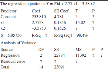
(a) Fill in the missing quantities. You may use bounds for the P-values.
(b) What conclusions can you draw about the significance of regression?
(c) What conclusions can you draw about the contributions of the individual regressors to the model?
12-30. You have fit a regression model with two regressors to a data set that has 20 observations. The total sum of squares is 1000 and the model sum of squares is 750.
(a) What is the value of R2 for this model?
(b) What is the adjusted R2 for this model?
(c) What is the value of the F-statistic for testing the significance of regression? What conclusions would you draw about this model if α = 0.05? What if α = 0.01?
(d) Suppose that you add a third regressor to the model and as a result, the model sum of squares is now 785. Does it seem to you that adding this factor has improved the model?
![]() 12-31. Consider the regression model fit to the soil shear strength data in Exercise 12-5.
12-31. Consider the regression model fit to the soil shear strength data in Exercise 12-5.
(a) Test for significance of regression using α = 0.05. What is the P-value for this test?
(b) Construct the t-test on each regression coefficient. What are your conclusions, using α = 0.05? Calculate P-values.
![]() 12-32. Consider the absorption index data in Exercise 12-6. The total sum of squares for y is SST = 742.00.
12-32. Consider the absorption index data in Exercise 12-6. The total sum of squares for y is SST = 742.00.
(a) Test for significance of regression using α = 0.01. What is the P-value for this test?
(b) Test the hypothesis H0: β1 = 0 versus H1: β1 ≠ 0 using α = 0.01. What is the P-value for this test?
(c) What conclusion can you draw about the usefulness of x1 as a regressor in this model?
12-33. ![]() A regression model Y = β0 + β1x1 + β2x2 + β3x3 +
A regression model Y = β0 + β1x1 + β2x2 + β3x3 + ![]() as been fit to a sample of n = 25 observations. The calculated t-ratios
as been fit to a sample of n = 25 observations. The calculated t-ratios ![]() j/se(
j/se(![]() j), j = 1, 2, 3 are as follows: for β1, t0 = 4.82, for β2, t0 = 8.21, and for β3, t0 = 0.98.
j), j = 1, 2, 3 are as follows: for β1, t0 = 4.82, for β2, t0 = 8.21, and for β3, t0 = 0.98.
(a) Find P-values for each of the t-statistics.
(b) Using α = 0.05, what conclusions can you draw about the regressor x3? Does it seem likely that this regressor contributes significantly to the model?
12-34. Consider the electric power consumption data in Exercise 12-10.
![]() (a) Test for significance of regression using α = 0.05. What is the P-value for this test?
(a) Test for significance of regression using α = 0.05. What is the P-value for this test?
(b) Use the t-test to assess the contribution of each regressor to the model. Using α = 0.05, what conclusions can you draw?
12-35. Consider the gasoline mileage data in Exercise 12-11.
![]() (a) Test for significance of regression using α = 0.05. What conclusions can you draw?
(a) Test for significance of regression using α = 0.05. What conclusions can you draw?
(b) Find the t-test statistic for each regressor. Using α = 0.05., what conclusions can you draw? Does each regressor contribute to the model?
![]() 12-36. Consider the wire bond pull strength data in Exercise 12-12.
12-36. Consider the wire bond pull strength data in Exercise 12-12.
(a) Test for significance of regression using α = 0.05. Find the P-value for this test. What conclusions can you draw?
(b) Calculate the t-test statistic for each regression coefficient. Using α = 0.05, what conclusions can you draw? Do all variables contribute to the model?
![]()
12-37. Reconsider the semiconductor data in Exercise 12-13.
(a) Test for significance of regression using α = 0.05. What conclusions can you draw?
(b) Calculate the t-test statistic and P-value for each regression coefficient. Using α = 0.05, what conclusions can you draw?
12-38. Consider the regression model fit to the arsenic data in Exercise 12-16. Use arsenic in nails as the response and age, drink use, and cook use as the regressors.
![]()
(a) Test for significance of regression using α = 0.05. What is the P-value for this test?
(b) Construct a t-test on each regression coefficient. What conclusions can you draw about the variables in this model? Use α = 0.05.
![]()
12-39. Consider the regression model fit to the X-ray inspection data in Exercise 12-15. Use rads as the response.
(a) Test for significance of regression using α = 0.05. What is the P-value for this test?
(b) Construct a t-test on each regression coefficient. What conclusions can you draw about the variables in this model? Use α = 0.05.
![]()
12-40. Consider the regression model fit to the nisin extraction data in Exercise 12-18. Use nisin extraction as the response.
(a) Test for significance of regression using α = 0.05. What is the P-value for this test?
(b) Construct a t-test on each regression coefficient. What conclusions can you draw about the variables in this model? Use α = 0.05.
(c) Comment on the effect of a small sample size to the tests in the previous parts.
12-41. Consider the regression model fit to the gray range modulation data in Exercise 12-19. Use the useful range as the response.
![]()
(a) Test for significance of regression using α = 0.05. What is the P-value for this test?
(b) Construct a t-test on each regression coefficient. What conclusions can you draw about the variables in this model? Use α = 0.05.
![]()
12-42. Consider the regression model fit to the stack loss data in Exercise 12-20. Use stack loss as the response.
(a) Test for significance of regression using α = 0.05. What is the P-value for this test?
(b) Construct a t-test on each regression coefficient. What conclusions can you draw about the variables in this model? Use α = 0.05.
![]()
12-43. Consider the NFL data in Exercise 12-21.
(a) Test for significance of regression using α = 0.05. What is the P-value for this test?
(b) Conduct the t-test for each regression coefficient. Using α = 0.05, what conclusions can you draw about the variables in this model?
(c) Find the amount by which the regressor x2 (TD percentage) increases the regression sum of squares, and conduct an F-test for H0: β2 = 0 versus H1: β2 ≠ 0 using α = 0.05. What is the P-value for this test? What conclusions can you draw?
![]() 12-44.
12-44. ![]() Go Tutorial Exercise 12-14 presents data on heat-treating gears.
Go Tutorial Exercise 12-14 presents data on heat-treating gears.
(a) Test the regression model for significance of regression. Using α = 0.05, find the P-value for the test and draw conclusions.
(b) Evaluate the contribution of each regressor to the model using the t-test with α = 0.05.
(c) Fit a new model to the response PITCH using new regressors x1 = SOAKTIME × SOAKPCT and x2 = DIFFTIME × DIFFPCT.
(d) Test the model in part (c) for significance of regression using α = 0.05. Also calculate the t-test for each regressor and draw conclusions.
(e) Estimate σ2 for the model from part (c) and compare this to the estimate of σ2 for the model in part (a). Which estimate is smaller? Does this offer any insight regarding which model might be preferable?
![]() 12-45. Consider the bearing wear data in Exercise 12-23.
12-45. Consider the bearing wear data in Exercise 12-23.
(a) For the model with no interaction, test for significance of regression using α = 0.05. What is the P-value for this test? What are your conclusions?
(b) For the model with no interaction, compute the t-statistics for each regression coefficient. Using α = 0.05, what conclusions can you draw?
(c) For the model with no interaction, use the extra sum of squares method to investigate the usefulness of adding x2 = load to a model that already contains x1 = oil viscosity. Use α = 0.05.
(d) Refit the model with an interaction term. Test for significance of regression using α = 0.05.
(e) Use the extra sum of squares method to determine whether the interaction term contributes significantly to the model. Use α = 0.05.
(f) Estimate σ2 for the interaction model. Compare this to the estimate of σ2 from the model in part (a).
![]()
12-46. Data on National Hockey League team performance were presented in Exercise 12-22.
(a) Test the model from this exercise for significance of regression using α = 0.05. What conclusions can you draw?
(b) Use the t-test to evaluate the contribution of each regressor to the model. Does it seem that all regressors are necessary? Use α = 0.05.
(c) Fit a regression model relating the number of games won to the number of goals for and the number of power play goals for. Does this seem to be a logical choice of regressors, considering your answer to part (b)? Test this new model for significance of regression and evaluate the contribution of each regressor to the model using the t-test. Use α = 0.05.
![]()
12-47. Data from a hospital patient satisfaction survey were presented in Exercise 12-9.
(a) Test the model from this exercise for significance of regression. What conclusions can you draw if α = 0.05? What if α = 0.01?
(b) Test the contribution of the individual regressors using the t-test. Does it seem that all regressors used in the model are really necessary?
![]()
12-48. Data from a hospital patient satisfaction survey were presented in Exercise 12-9.
(a) Fit a regression model using only the patient age and severity regressors. Test the model from this exercise for significance of regression. What conclusions can you draw if α = 0.05? What if α = 0.01?
(b) Test the contribution of the individual regressors using the t-test. Does it seem that all regressors used in the model are really necessary?
(c) Find an estimate of the error variance σ2. Compare this estimate of σ2 with the estimate obtained from the model containing the third regressor, anxiety. Which estimate is smaller? Does this tell you anything about which model might be preferred?
12-3 Confidence Intervals In Multiple Linear Regression
12-3.1 CONFIDENCE INTERVALS ON INDIVIDUAL REGRESSION COEFFICIENTS
In multiple regression models, is often useful to construct confidence interval estimates for the regression coefficients {βj}. The development of a procedure for obtaining these confidence intervals requires that the errors {![]() i} are normally and independently distributed with mean zero and variance σ2. This is the same assumption required in hypothesis testing. Therefore, the observations {Yi} are normally and independently distributed with mean β0 +
i} are normally and independently distributed with mean zero and variance σ2. This is the same assumption required in hypothesis testing. Therefore, the observations {Yi} are normally and independently distributed with mean β0 + ![]() and variance σ2. Because the least squares estimator
and variance σ2. Because the least squares estimator ![]() is a linear combination of the observations, it follows that
is a linear combination of the observations, it follows that ![]() is normally distributed with mean vector β and covariance atrix σ2(X′X)−1. Then each of the statistics
is normally distributed with mean vector β and covariance atrix σ2(X′X)−1. Then each of the statistics
![]()
has a t distribution with n − p degrees of freedom where Cjj is the jjth element of the (X′X)−1 matrix, and ![]() 2 is the estimate of the error variance, obtained from Equation 12-16. This leads to the following 100(1 − α)% confidence interval for the regression coefficient βj, j = 0, 1,..., k.
2 is the estimate of the error variance, obtained from Equation 12-16. This leads to the following 100(1 − α)% confidence interval for the regression coefficient βj, j = 0, 1,..., k.
A 100(1 − α)% confidence interval on the regression coefficient βj, j = 0, 1,..., k in the multiple linear regression model is given by
![]()
Because ![]() is the standard error of the regression coefficient
is the standard error of the regression coefficient ![]() j, we would also write the CI formula as
j, we would also write the CI formula as ![]() j − tα/2,n−p se(βj) ≤ βj ≤
j − tα/2,n−p se(βj) ≤ βj ≤ ![]() j + tα/2,n−pse(βj).
j + tα/2,n−pse(βj).
Example 12-7 Wire Bond Strength Confidence Interval We will construct a 95% confidence interval on the parameter β1 in the wire bond pull strength problem. The point estimate of β1 is ![]() 1 = 2.74427, and the diagonal element of (X′X)−1 corresponding to β1 is C11 = 0.001671. The estimate of σ2 is
1 = 2.74427, and the diagonal element of (X′X)−1 corresponding to β1 is C11 = 0.001671. The estimate of σ2 is ![]() 2 = 5.2352, and t0.025,22 = 2.074. Therefore, the 95% CI on β1 is computed from Equation 12-35 as
2 = 5.2352, and t0.025,22 = 2.074. Therefore, the 95% CI on β1 is computed from Equation 12-35 as
![]()
which reduces to
![]()
Also, computer software can be used to help calculate this confidence interval. From the regression output in Table 10-4, ![]() 1 = 2.74427 and the standard error of
1 = 2.74427 and the standard error of ![]() 1 = 0.0935. This standard error is the multiplier of the t-table constant in the confidence interval. That is, 0.0935 =
1 = 0.0935. This standard error is the multiplier of the t-table constant in the confidence interval. That is, 0.0935 = ![]() . Consequently, all the numbers are available from the computer output to construct the interval, which is the typical method used in practice.
. Consequently, all the numbers are available from the computer output to construct the interval, which is the typical method used in practice.
12-3.2 CONFIDENCE INTERVAL ON THE MEAN RESPONSE
We may also obtain a confidence interval on the mean response at a particular point, say, x01, x02,..., x0k. To estimate the mean response at this point, define the vector
The mean response at this point is E(Y|x0) = μY|x0 = x′0β, which is estimated by
![]()
This estimator is unbiased, because E(x0′ ![]() ) = x0′ β = E(Y|x0) = μY|x0 and the variance of
) = x0′ β = E(Y|x0) = μY|x0 and the variance of ![]() Y|x0 is
Y|x0 is
![]()
A 100(1 − α)% CI on μY|x0 can be constructed from the statistic
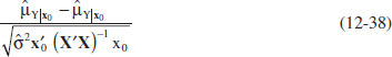
Confidence Interval on the Mean Response
For the multiple linear regression model, a 100(1 − α)% confidence interval on the mean response at the point x01, x02,...,x0k is
![]()
Equation 12-39 is a CI about the regression plane (or hyperplane). It is the multiple regression generalization of Equation 11-32.
Example 12-8 Wire Bond Strength Confidence Interval on the Mean Response The engineer in Example 12-1 would like to construct a 95% CI on the mean pull strength for a wire bond with wire length x1 = 8 and die height x2 = 275. Therefore,

The estimated mean response at this point is found from Equation 12-36 as

The variance of ![]() Y|x0 is estimated by
Y|x0 is estimated by
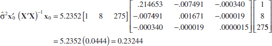
Therefore, a 95% CI on the mean pull strength at this point is found from Equation 12-39 as
![]()
which reduces to
![]()
Some computer software will provide estimates of the mean for a point of interest x0 and the associated CI. Table 12-4 shows the computer output for Example 12-8. Both the estimate of the mean and the 95% CI are provided.
12-4 Prediction of New Observations
A regression model can be used to predict new or future observations on the response variable Y corresponding to particular values of the independent variables, say, x01, x02,...,x0k. If x′0 = [1x01, x02...x0k], a point estimate of the future observation Y0 at the point x01, x02,...,x0k is
![]()
Prediction Interval
A 100(1 − α)% prediction interval on a future observation is
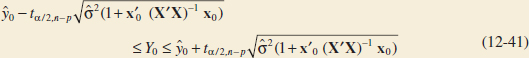
This prediction interval is a generalization of the prediction interval given in Equation 11-33 for a future observation in simple linear regression. If we compare the prediction interval Equation 12-41 with the expression for the confidence interval on the mean, Equation 12-39, you will observe that the prediction interval is always wider than the confidence interval. The confidence interval expresses the error in estimating the mean of a distribution, and the prediction interval expresses the error in predicting a future observation from the distribution at the point x0. This must include the error in estimating the mean at that point as well as the inherent variability in the random variable Y at the same value x = x0.

FIGURE 12-5 An example of extrapolation in multiple regression
Also, we might want to predict the mean of several values of Y, say m, all at the same value x = x0. Because the variance of a sample mean is σ2/m, Equation 12-41 is modified as follows. Replace the constant 1 under the square root with 1/m to reflect the lower variability in the mean of m observations. This results in a narrower interval.
In predicting new observations and in estimating the mean response at a given point x01, x02,...,x0k, we must be careful about extrapolating beyond the region containing the original observations. It is very possible that a model that fits well in the region of the original data will no longer fit well outside of that region. In multiple regression, inadvertently extrapolating is often easy because the levels of the variables (xi1, xi2,...,xik), i = 1,2,...,n, jointly define the region containing the data. As an example, consider Fig. 12-5, which illustrates the region containing the observations for a two-variable regression model. Note that the point (x01, x02) lies within the ranges of both regressor variables x1 and x2, but it is outside the region that is actually spanned by the original observations. This is sometimes called a hidden extrapolation. Either predicting the value of a new observation or estimating the mean response at this point is an extrapolation of the original regression model.
Example 12-9 Wire Bond Strength Confidence Interval Suppose that the engineer in Example 12-1 wishes to construct a 95% prediction interval on the wire bond pull strength when the wire length is x1 = 8 and the die height is x2 = 275. Note that x′0 = [1 8 275], and the point estimate of the pull strength is ![]() 0 = x′0
0 = x′0![]() = 27.66. Also, in Example 12-8, we calculated x′0(X′X)−1 x0 = 0.04444. Therefore, from Equation 12-41 we have
= 27.66. Also, in Example 12-8, we calculated x′0(X′X)−1 x0 = 0.04444. Therefore, from Equation 12-41 we have
![]()
and the 95% prediction interval is
![]()
Notice that the prediction interval is wider than the confidence interval on the mean response at the same point, calculated in Example 12-8. The computer output in Table 12-4 also displays this prediction interval.
EXERCISES FOR SECTION 12-3 AND 12-4
![]() Problem available in WileyPLUS at instructor's discretion.
Problem available in WileyPLUS at instructor's discretion.
![]() Go Tutorial Tutoring problem available in WileyPLUS at instructor's discretion.
Go Tutorial Tutoring problem available in WileyPLUS at instructor's discretion.
![]() 12-49 Using the regression model from Exercise 12-1,
12-49 Using the regression model from Exercise 12-1,
(a) Find a 95% confidence interval for the coefficient of height.
(b) Find a 95% confidence interval for the mean percent of body fat for a man with a height of 72in and waist of 34in.
(c) Find a 95% prediction interval for the percent of body fat for a man with the same height and waist as in part (b).
(d) Which interval is wider, the confidence interval or the prediction interval? Explain briefly.
(e) Given your answer to part (c), do you believe that this is a useful model for predicting body fat? Explain briefly.
![]() 12-50 Using the regression from Exercise 12-2,
12-50 Using the regression from Exercise 12-2,
(a) Find a 95% confidence interval for the coefficient of hourly 1 test.
(b) Find a 95% confidence interval for the mean final grade for students who score 80 on the first test and 85 on the second.
(c) Find a 95% prediction interval for a student with the same grades as in part (b).
![]() 12-51 Referring to the regression model from Exercise 12-3,
12-51 Referring to the regression model from Exercise 12-3,
(a) Find a 95% confidence interval for the coefficient of spending on higher education.
(b) Is zero in the confidence interval you found in part (a)? What does that fact imply about the coefficient of higher education?
(c) Find a 95% prediction interval for a state that has $1 per $1000 in venture capital, spends $10,000 per student on funding for major research universities, and spends 0.5% of its GDP on higher education.
![]() 12-52 Use the second-order polynomial regression model from Exercise 12-4,
12-52 Use the second-order polynomial regression model from Exercise 12-4,
(a) Find a 95% confidence interval on both the first-order and the second-order term in this model.
(b) Is zero in the confidence interval you found for the second-order term in part (a)? What does that fact tell you about the contribution of the second-order term to the model?
(c) Refit the model with only the first-order term. Find a 95% confidence interval on this term. Is this interval longer or shorter than the confidence interval that you found on this term in part (a)?
![]() 12-53. Consider the regression model fit to the shear strength of soil in Exercise 12-5.
12-53. Consider the regression model fit to the shear strength of soil in Exercise 12-5.
(a) Calculate 95% confidence intervals on each regression coefficient.
(b) Calculate a 95% confidence interval on mean strength when x1 = 18 ft and x2 = 43%.
(c) Calculate 95% prediction interval on strength for the same values of the regressors used in the previous part.
![]() 12-54. Consider the soil absorption data in Exercise 12-6.
12-54. Consider the soil absorption data in Exercise 12-6.
(a) Find 95% confidence intervals on the regression coefficients.
(b) Find a 95% confidence interval on mean soil absorption index when x1 = 200 and x2 = 50.
(c) Find a 95% prediction interval on the soil absorption index when x1 = 200 and x2 = 50.
12-55. Consider the semiconductor data in Exercise 12-13.
(a) Find 99% confidence intervals on the regression coefficients.
![]()
(b) Find a 99% prediction interval on HFE when x1 = 14.5, x2 = 220, and x3 = 5.0
(c) Find a 99% confidence interval on mean HFE when x1 = 14.5, x2 = 220, and x3 = 5.0.
![]()
12-56. ![]() Consider the electric power consumption data in Exercise 12-10.
Consider the electric power consumption data in Exercise 12-10.
(a) Find 95% confidence intervals on β1, β2, β3, and β4.
(b) Find a 95% confidence interval on the mean of Y when x1 = 75, x2 = 24, x3 = 90, and x4 = 98.
(c) Find a 95% prediction interval on the power consumption when x1 = 75, x2 = 24, x3 = 90, and x4 = 98.
![]()
12-57. Consider the bearing wear data in Exercise 12-23.
(a) Find 99% confidence intervals on β1 and β2.
(b) Recompute the confidence intervals in part (a) after the interaction term x1x2 is added to the model. Compare the lengths of these confidence intervals with those computed in part (a). Do the lengths of these intervals provide any information about the contribution of the interaction term in the model?
12-58. ![]() Consider the wire bond pull strength data in Exercise 12-12.
Consider the wire bond pull strength data in Exercise 12-12.
(a) Find 95% confidence interval on the regression coefficients.
![]()
(b) Find a 95% confidence interval on mean pull strength when x2 = 20, x3 = 30, x4 = 90, and x5 = 2.0.
(c) Find a 95% prediction interval on pull strength when x2 = 20, x3 = 30, x4 = 90, and x5 = 2.0.
![]()
12-59. Consider the regression model fit to the X-ray inspection data in Exercise 12-15. Use rads as the response.
(a) Calculate 95% confidence intervals on each regression coefficient.
(b) Calculate a 99% confidence interval on mean rads at 15 milliamps and 1 second on exposure time.
(c) Calculate a 99% prediction interval on rads for the same values of the regressors used in the part (b).
![]()
12-60. ![]() Consider the regression model fit to the arsenic data in Exercise 12-16. Use arsenic in nails as the response and age, drink use, and cook use as the regressors.
Consider the regression model fit to the arsenic data in Exercise 12-16. Use arsenic in nails as the response and age, drink use, and cook use as the regressors.
(a) Calculate 99% confidence intervals on each regression coefficient.
(b) Calculate a 99% confidence interval on mean arsenic concentration in nails when age = 30, drink use = 4, and cook use = 4.
(c) Calculate a prediction interval on arsenic concentration in nails for the same values of the regressors used in part (b).
12-61. ![]() Go Tutorial Consider the regression model fit to the coal and limestone mixture data in Exercise 12-17. Use density as the response.
Go Tutorial Consider the regression model fit to the coal and limestone mixture data in Exercise 12-17. Use density as the response.
![]()
(a) Calculate 90% confidence intervals on each regression coefficient.
(b) Calculate a 90% confidence interval on mean density when the dielectric constant = 2.3 and the loss factor = 0.025.
(c) Calculate a prediction interval on density for the same values of the regressors used in part (b).
12-62. ![]() Consider the regression model fit to the nisin extraction data in Exercise 12-18.
Consider the regression model fit to the nisin extraction data in Exercise 12-18.
![]()
(a) Calculate 95% confidence intervals on each regression coefficient.
(b) Calculate a 95% confidence interval on mean nisin extraction when x1 = 15.5 and x2 = 16.
(c) Calculate a prediction interval on nisin extraction for the same values of the regressors used in part (b).
(d) Comment on the effect of a small sample size to the widths of these intervals.
12-63. Consider the regression model fit to the gray range modulation data in Exercise 12-19. Use the useful range as the response.
![]()
(a) Calculate 99% confidence intervals on each regression coefficient.
(b) Calculate a 99% confidence interval on mean useful range when brightness = 70 and contrast = 80.
(c) Calculate a prediction interval on useful range for the same values of the regressors used in part (b).
(d) Calculate a 99% confidence interval and a 99% a prediction interval on useful range when brightness = 50 and contrast = 25. Compare the widths of these intervals to those calculated in parts (b) and (c). Explain any differences in widths.
12-64. Consider the stack loss data in Exercise 12-20.
![]()
(a) Calculate 95% confidence intervals on each regression coefficient.
(b) Calculate a 95% confidence interval on mean stack loss when x1 = 80, x2 = 25 and x3 = 90.
(c) Calculate a prediction interval on stack loss for the same values of the regressors used in part (b).
(d) Calculate a 95% confidence interval and a 95% prediction interval on stack loss when x1 = 80, x2 = 19, and x3 = 93. Compare the widths of these intervals to those calculated in parts (b) and (c). Explain any differences in widths.
![]()
12-65. ![]() Consider the NFL data in Exercise 12-21.
Consider the NFL data in Exercise 12-21.
(a) Find 95% confidence intervals on the regression coefficients.
(b) What is the estimated standard error of ![]() Y|x0 when the percentage of completions is 60%, the percentage of TDs is 4%, and the percentage of interceptions is 3%.
Y|x0 when the percentage of completions is 60%, the percentage of TDs is 4%, and the percentage of interceptions is 3%.
(c) Find a 95% confidence interval on the mean rating when the percentage of completions is 60%, the percentage of TDs is 4%, and the percentage of interceptions is 3%.
![]()
12-66. ![]() Consider the heat-treating data from Exercise 12-14.
Consider the heat-treating data from Exercise 12-14.
(a) Find 95% confidence intervals on the regression coefficients.
(b) Find a 95% confidence interval on mean PITCH when TEMP = 1650, SOAKTIME = 1.00, SOAKPCT = 1.10, DIFFTIME = 1.00, and DIFFPCT = 0.80.
(c) Fit a model to PITCH using regressors x1 = SOAKTIME × SOAKPCT and x2 = DIFFTIME × DIFFPCT. Using the model with regressors x1 and x2, find a 95% confidence interval on mean PITCH when SOAKTIME = 1.00, SOAKPCT = 1.10, DIFFTIME = 1.00, and DIFFPCT = 0.80.
(d) Compare the length of this confidence interval with the length of the confidence interval on mean PITCH at the same point from part (b), which used an additive model in SOAKTIME, SOAKPCT, DIFFTIME, and DIFFPCT. Which confidence interval is shorter? Does this tell you anything about which model is preferable?
![]()
12-67. ![]() Consider the gasoline mileage data in Exercise 12-11.
Consider the gasoline mileage data in Exercise 12-11.
(a) Find 99% confidence intervals on the regression coefficients.
(b) Find a 99% confidence interval on the mean of Y for the regressor values in the first row of data.
(c) Fit a new regression model to these data using cid, etw, and axle as the regressors. Find 99% confidence intervals on the regression coefficients in this new model.
(d) Compare the lengths of the confidence intervals from part (c) with those found in part (a). Which intervals are longer? Does this offer any insight about which model is preferable?
12-68. Consider the NHL data in Exercise 12-22.
(a) Find a 95% confidence interval on the regression coefficient for the variable GF.
(b) Fit a simple linear regression model relating the response variable to the regressor GF.
![]()
(c) Find a 95% confidence interval on the slope for the simple linear regression model from part (b).
(d) Compare the lengths of the two confidence intervals computed in parts (a) and (c). Which interval is shorter? Does this tell you anything about which model is preferable?
12-5 Model Adequacy Checking
12-5.1 RESIDUAL ANALYSIS
The residuals from the multiple regression model, defined by ei = yi − ![]() i, play an important role in judging model adequacy just as they do in simple linear regression. As noted in Section 11-7.1, several residual plots are often useful; these are illustrated in Example 12-10. It is also helpful to plot the residuals against variables not presently in the model that are possible candidates for inclusion. Patterns in these plots may indicate that the model may be improved by adding the candidate variable.
i, play an important role in judging model adequacy just as they do in simple linear regression. As noted in Section 11-7.1, several residual plots are often useful; these are illustrated in Example 12-10. It is also helpful to plot the residuals against variables not presently in the model that are possible candidates for inclusion. Patterns in these plots may indicate that the model may be improved by adding the candidate variable.
Example 12-10 Wire Bond Strength Residuals The residuals for the model from Example 12-1 are shown in Table 12-3. A normal probability plot of these residuals is shown in Fig. 12-6. No severe deviations from normality are obviously apparent, although the two largest residuals (e15 = 5.84 and e17 = 4.33) do not fall extremely close to a straight line drawn through the remaining residuals.
The standardized residuals
Standardized Residual
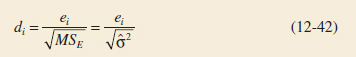
are often more useful than the ordinary residuals when assessing residual magnitude. For the wire bond strength example, the standardized residuals corresponding to e15 and e17 are d15 = 5.84 / ![]() = 2.55 and d17 = 4.33 /
= 2.55 and d17 = 4.33 / ![]() = 1.89, and they do not seem unusually large. Inspection of the data does not reveal any error in collecting observations 15 and 17, nor does it produce any other reason to discard or modify these two points.
= 1.89, and they do not seem unusually large. Inspection of the data does not reveal any error in collecting observations 15 and 17, nor does it produce any other reason to discard or modify these two points.
The residuals are plotted against ![]() in Fig. 12-7, and against x1 and x2 in Figs. 12-8 and 12-9, respectively.* The two largest residuals, e15 and e17, are apparent. Figure 12-8 gives some indication that the model underpredicts the pull strength for assemblies with short wire length (x1 ≤ 6) and long wire length (x1 ≥ 15) and overpredicts the strength for assemblies with intermediate wire length (7 ≤ x1 ≤ 14). The same impression is obtained from Fig. 12-7. Either the relationship between strength and wire length is not linear (requiring that a term involving
in Fig. 12-7, and against x1 and x2 in Figs. 12-8 and 12-9, respectively.* The two largest residuals, e15 and e17, are apparent. Figure 12-8 gives some indication that the model underpredicts the pull strength for assemblies with short wire length (x1 ≤ 6) and long wire length (x1 ≥ 15) and overpredicts the strength for assemblies with intermediate wire length (7 ≤ x1 ≤ 14). The same impression is obtained from Fig. 12-7. Either the relationship between strength and wire length is not linear (requiring that a term involving ![]() , say, be added to the model) or other regressor variables not presently in the model affected the response.
, say, be added to the model) or other regressor variables not presently in the model affected the response.
In the wire bond strength example, we used the standardized residuals di = ei / ![]() as a measure of residual magnitude. Some analysts prefer to plot standardized residuals instead of ordinary residuals because the standardized residuals are scaled so that their standard deviation is approximately unity. Consequently, large residuals (that may indicate possible outliers or unusual observations) will be more obvious from inspection of the residual plots.
as a measure of residual magnitude. Some analysts prefer to plot standardized residuals instead of ordinary residuals because the standardized residuals are scaled so that their standard deviation is approximately unity. Consequently, large residuals (that may indicate possible outliers or unusual observations) will be more obvious from inspection of the residual plots.
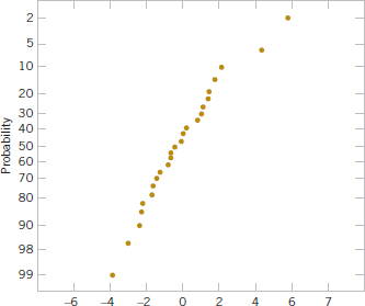
FIGURE 12-6 Normal probability plot of residuals.

FIGURE 12-7 Plot of residuals against ![]() .
.

FIGURE 12-8 Plot of residuals against x1.

FIGURE 12-9 Plot of residuals against x2.
Many regression computer programs compute other types of scaled residuals. One of the most popular are the studentized residuals
Studentized Residual
where hii is the ith diagonal element of the matrix
![]()
The H matrix is sometimes called the “hat” matrix, because
![]()
Thus, H transforms the observed values of y into a vector of fitted values ![]() .
.
Because each row of the matrix X corresponds to a vector, say x′i =[1, xi1, xi2,..., xik], another way to write the diagonal elements of the hat matrix is
Diagonal Elements of Hat Matrix
![]()
Note that apart from σ2, hii is the variance of the fitted value ![]() i. The quantities hii were used in the computation of the confidence interval on the mean response in Section 12-3.2.
i. The quantities hii were used in the computation of the confidence interval on the mean response in Section 12-3.2.
Under the usual assumptions that the model errors are independently distributed with mean zero and variance σ2, we can show that the variance of the ith residual ei is
![]()
Furthermore, the hii elements must fall in the interval 0 < hii ≤ 1. This implies that the standardized residuals understate the true residual magnitude; thus, the studentized residuals would be a better statistic to examine in evaluating potential outliers.
To illustrate, consider the two observations identified in the wire bond strength data (Example 12-10) as having residuals that might be unusually large, observations 15 and 17. The standardized residuals are
![]()
Now h15,15 = 0.0737 and h17,17 = 0.2593, so the studentized residuals are
![]()
and
![]()
Notice that the studentized residuals are larger than the corresponding standardized residuals. However, the studentized residuals are still not so large as to cause us serious concern about possible outliers.
12-5.2 INFLUENTIAL OBSERVATIONS
When using multiple regression, we occasionally find that some subset of the observations is unusually influential. Sometimes these influential observations are relatively far away from the vicinity where the rest of the data were collected. A hypothetical situation for two variables is depicted in Fig. 12-10 in which one observation in x-space is remote from the rest of the data. The disposition of points in the x-space is important in determining the properties of the model. For example, point (xi1, xi2) in Fig. 12-10 may be very influential in determining R2, the estimates of the regression coefficients, and the magnitude of the error mean square.
We would like to examine the influential points to determine whether they control many model properties. If these influential points are “bad” points, or erroneous in any way, they should be eliminated. On the other hand, there may be nothing wrong with these points, but at least we would like to determine whether or not they produce results consistent with the rest of the data. In any event, even if an influential point is a valid one, if it controls important model properties, we would like to know this, because it could have an impact on the use of the model.
Montgomery, Peck, and Vining (2012) and Myers (1990) describe several methods for detecting influential observations. An excellent diagnostic is the distance measure developed by Dennis R. Cook. This is a measure of the squared distance between the usual least squares estimate of β based on all n observations and the estimate obtained when the th point is removed, say, ![]() (i). The Cook's distance measure is
(i). The Cook's distance measure is
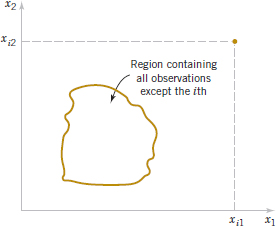
FIGURE 12-10 A point that is remote in x-space.
Clearly, if the ith point is influential, its removal will result in ![]() (i) changing considerably from the value
(i) changing considerably from the value ![]() . Thus, a large value of Di implies that the ith point is influential. The statistic Di is actually computed using
. Thus, a large value of Di implies that the ith point is influential. The statistic Di is actually computed using
Cook's Distance Formula

From Equation 12-45, we see that Di consists of the squared studentized residual, which reflects how well the model fits the ith observation yi [recall that ri = ei/![]() ] and a component that measures how far that point is from the rest of the data [hii / (1 − hii) is a measure of the distance of the ith point from the centroid of the remaining n − 1 points]. A value of Di > 1 would indicate that the point is influential. Either component of Di (or both) may contribute to a large value.
] and a component that measures how far that point is from the rest of the data [hii / (1 − hii) is a measure of the distance of the ith point from the centroid of the remaining n − 1 points]. A value of Di > 1 would indicate that the point is influential. Either component of Di (or both) may contribute to a large value.
Example 12-11 Wire Bond Strength Cook's Distances Table 12-8 lists the values of the hat matrix diagonals hii and Cook's distance measure Di for the wire bond pull strength data in Example 12-1. To illustrate the calculations, consider the first observation:
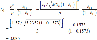
The Cook distance measure Di does not identify any potentially influential observations in the data, for no value of Di exceeds unity.
![]() TABLE • 12-8 Influence Diagnostics for the Wire Bond Pull Strength Data
TABLE • 12-8 Influence Diagnostics for the Wire Bond Pull Strength Data
EXERCISES FOR SECTION 12-5
![]() Problem available in WileyPLUS at instructor's discretion.
Problem available in WileyPLUS at instructor's discretion.
![]() Go Tutorial Tutoring problem available in WileyPLUS at instructor's discretion.
Go Tutorial Tutoring problem available in WileyPLUS at instructor's discretion.
![]() 12-69. Consider the gasoline mileage data in Exercise 12-11.
12-69. Consider the gasoline mileage data in Exercise 12-11.
(a) What proportion of total variability is explained by this model?
(b) Construct a normal probability plot of the residuals and comment on the normality assumption.
(c) Plot residuals versus ![]() and versus each regressor. Discuss these residual plots.
and versus each regressor. Discuss these residual plots.
(d) Calculate Cook's distance for the observations in this data set. Are any observations influential?
![]()
12-70. Consider the electric power consumption data in Exercise 12-10.
(a) Calculate R2 for this model. Interpret this quantity.
(b) Plot the residuals versus ![]() and versus each regressor. Interpret this plot.
and versus each regressor. Interpret this plot.
(c) Construct a normal probability plot of the residuals and comment on the normality assumption.
12-71. Consider the regression model for the NFL data in Exercise 12-21.
![]()
(a) What proportion of total variability is explained by this model?
(b) Construct a normal probability plot of the residuals. What conclusion can you draw from this plot?
(c) Plot the residuals versus ![]() and versus each regressor, and comment on model adequacy.
and versus each regressor, and comment on model adequacy.
(d) Are there any influential points in these data?
12-72. ![]() Consider the regression model for the heat-treating data in Exercise 12-14.
Consider the regression model for the heat-treating data in Exercise 12-14.
![]()
(a) Calculate the percent of variability explained by this model.
(b) Construct a normal probability plot for the residuals. Comment on the normality assumption.
(c) Plot the residuals versus ![]() and interpret the display.
and interpret the display.
(d) Calculate Cook's distance for each observation and provide an interpretation of this statistic.
12-73. ![]() Consider the regression model fit to the X-ray inspection data in Exercise 12-15. Use rads as the response.
Consider the regression model fit to the X-ray inspection data in Exercise 12-15. Use rads as the response.
![]()
(a) What proportion of total variability is explained by this model?
(b) Construct a normal probability plot of the residuals. What conclusion can you draw from this plot?
(c) Plot the residuals versus ![]() and versus each regressor, and comment on model adequacy.
and versus each regressor, and comment on model adequacy.
(d) Calculate Cook's distance for the observations in this data set. Are there any influential points in these data?
![]()
12-74. ![]() Consider the regression model fit to the arsenic data in Exercise 12-16. Use arsenic in nails as the response and age, drink use, and cook use as the regressors.
Consider the regression model fit to the arsenic data in Exercise 12-16. Use arsenic in nails as the response and age, drink use, and cook use as the regressors.
(a) What proportion of total variability is explained by this model?
(b) Construct a normal probability plot of the residuals. What conclusion can you draw from this plot?
(c) Plot the residuals versus ![]() and versus each regressor, and comment on model adequacy.
and versus each regressor, and comment on model adequacy.
(d) Calculate Cook's distance for the observations in this data set. Are there any influential points in these data?
12-75. ![]() Consider the regression model fit to the coal and limestone mixture data in Exercise 12-17. Use density as the response.
Consider the regression model fit to the coal and limestone mixture data in Exercise 12-17. Use density as the response.
(a) What proportion of total variability is explained by this model?
![]()
(b) Construct a normal probability plot of the residuals. What conclusion can you draw from this plot?
(c) Plot the residuals versus ![]() and versus each regressor, and comment on model adequacy.
and versus each regressor, and comment on model adequacy.
(d) Calculate Cook's distance for the observations in this data set. Are there any influential points in these data?
12-76. Consider the regression model fit to the nisin extraction data in Exercise 12-18.
![]()
(a) What proportion of total variability is explained by this model?
(b) Construct a normal probability plot of the residuals. What conclusion can you draw from this plot?
(c) Plot the residuals versus ![]() and versus each regressor, and comment on model adequacy.
and versus each regressor, and comment on model adequacy.
(d) Calculate Cook's distance for the observations in this data set. Are there any influential points in these data?
12-77. Consider the regression model fit to the gray range modulation data in Exercise 12-19. Use the useful range as the response.
![]()
(a) What proportion of total variability is explained by this model?
(b) Construct a normal probability plot of the residuals. What conclusion can you draw from this plot?
(c) Plot the residuals versus ![]() and versus each regressor, and comment on model adequacy.
and versus each regressor, and comment on model adequacy.
(d) Calculate Cook's distance for the observations in this data set. Are there any influential points in these data?
12-78. Consider the stack loss data in Exercise 12-20.
![]()
(a) What proportion of total variability is explained by this model?
(b) Construct a normal probability plot of the residuals. What conclusion can you draw from this plot?
(c) Plot the residuals versus ![]() and versus each regressor, and comment on model adequacy.
and versus each regressor, and comment on model adequacy.
(d) Calculate Cook's distance for the observations in this data set. Are there any influential points in these data?
12-79. Consider the bearing wear data in Exercise 12-23.
![]()
(a) Find the value of R2 when the model uses the regressors x1 and x2.
(b) What happens to the value of R2 when an interaction term x1x2 is added to the model? Does this necessarily imply that adding the interaction term is a good idea?
![]() 12-80. Fit a model to the response PITCH in the heat-treating data of Exercise 12-14 using new regressors x1 = SOAKTIME × SOAKPCT and x2 = DIFFTIME × DIFFPCT.
12-80. Fit a model to the response PITCH in the heat-treating data of Exercise 12-14 using new regressors x1 = SOAKTIME × SOAKPCT and x2 = DIFFTIME × DIFFPCT.
(a) Calculate the R2 for this model and compare it to the value of R2 from the original model in Exercise 12-14. Does this provide some information about which model is preferable?
(b) Plot the residuals from this model versus ![]() and on a normal probability scale. Comment on model adequacy.
and on a normal probability scale. Comment on model adequacy.
(c) Find the values of Cook's distance measure. Are any observations unusually influential?
12-81. Consider the semiconductor HFE data in Exercise 12-13.
![]()
(a) Plot the residuals from this model versus ![]() . Comment on the information in this plot.
. Comment on the information in this plot.
(b) What is the value of R2 for this model?
(c) Refit the model using log HFE as the response variable.
(d) Plot the residuals versus predicted log HFE for the model in part (c). Does this give any information about which model is preferable?
(e) Plot the residuals from the model in part (d) versus the regressor x3. Comment on this plot.
(f) Refit the model to log HFE using x1, x2, and 1/x3, as the regressors. Comment on the effect of this change in the model.
![]()
12-82. Consider the regression model for the NHL data from Exercise 12-22.
(a) Fit a model using as the only regressor.
(b) How much variability is explained by this model?
(c) Plot the residuals versus ![]() and comment on model adequacy.
and comment on model adequacy.
(d) Plot the residuals from part (a) versus PPGF, the points scored while in power play. Does this indicate that the model would be better if this variable were included?
12-83. The diagonal elements of the hat matrix are often used to denote leverage—that is, a point that is unusual in its location in the x-space and that may be influential. Generally, the ith point is called a leverage point if its hat diagonal hii exceeds 2p/n, which is twice the average size of all the hat diagonals. Recall that p = k + 1.
(a) Table 12-9 contains the hat diagonal for the wire bond pull strength data used in Example 12-5. Find the average size of these elements.
(b) Based on the preceding criterion, are there any observations that are leverage points in the data set?
12-6 Aspects of Multiple Regression Modeling
In this section, we briefly discuss several other aspects of building multiple regression models. For more extensive presentations of these topics and additional examples refer to Montgomery, Peck, and Vining (2012) and Myers (1990).
12-6.1 POLYNOMIAL REGRESSION MODELS
The linear model Y = Xβ + ![]() is a general model that can be used to fit any relationship that is linear in the unknown parameters β. This includes the important class of polynomial regression models. For example, the second-degree polynomial in one variable
is a general model that can be used to fit any relationship that is linear in the unknown parameters β. This includes the important class of polynomial regression models. For example, the second-degree polynomial in one variable
![]()
and the second-degree polynomial in two variables
![]()
are linear regression models.
Polynomial regression models are widely used when the response is curvilinear because the general principles of multiple regression can be applied. Example 12-12 illustrates some of the types of analyses that can be performed.
Example 12-12 Airplane Sidewall Panels Sidewall panels for the interior of an airplane are formed in a 1500-ton press. The unit manufacturing cost varies with the production lot size. The following data give the average cost per unit (in hundreds of dollars) for this product (y) and the production lot size (x). The scatter diagram, shown in Fig. 12-11, indicates that a second-order polynomial may be appropriate.

We will fit the model
![]()
The y vector, the model matrix X, and the β vector are as follows:

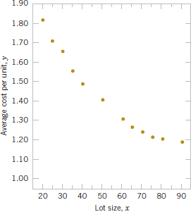
FIGURE 12-11 Data for Example 12-11.
![]() TABLE • 12-9 Test for Significance of Regression for the Second-Order Model in Example 12-12
TABLE • 12-9 Test for Significance of Regression for the Second-Order Model in Example 12-12
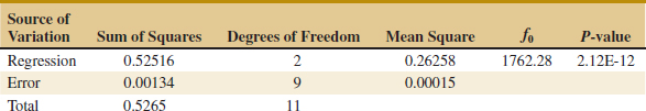
Solving the normal equations X′X![]() = X′y gives the fitted model
= X′y gives the fitted model
![]()
Conclusions: The test for significance of regression is shown in Table 12-9. Because f0 = 1762.3 is significant at 1%, we conclude that at least one of the parameters β1 and β11 is not zero. Furthermore, the standard tests for model adequacy do not reveal any unusual behavior, and we would conclude that this is a reasonable model for the sidewall panel cost data.
In fitting polynomials, we generally like to use the lowest-degree model consistent with the data. In this example, it would seem logical to investigate the possibility of dropping the quadratic term from the model. That is, we would like to test
![]()
The general regression significance test can be used to test this hypothesis. We need to determine the “extra sum of squares” due to β11, or
![]()
The sum of squares SSR(β1, β11|β0) = 0.52516 from Table 12-10. To find SSR(β1|β0), we fit a simple linear regression model to the original data, yielding
![]()
It can be easily verified that the regression sum of squares for this model is
![]()
Therefore, the extra sum of the squares due to β11, given that β1 and β0 are in the model, is
![]()
The analysis of variance with the test of H0: β11 = 0 incorporated into the procedure is displayed in Table 12-10. Note that the quadratic term contributes significantly to the model.
![]() TABLE • 12-10 Analysis of Variance for Example 12-12, Showing the Test for H0: β11 = 0
TABLE • 12-10 Analysis of Variance for Example 12-12, Showing the Test for H0: β11 = 0
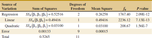
![]() TABLE • 12-11 Surface Finish Data for Example 12-13
TABLE • 12-11 Surface Finish Data for Example 12-13
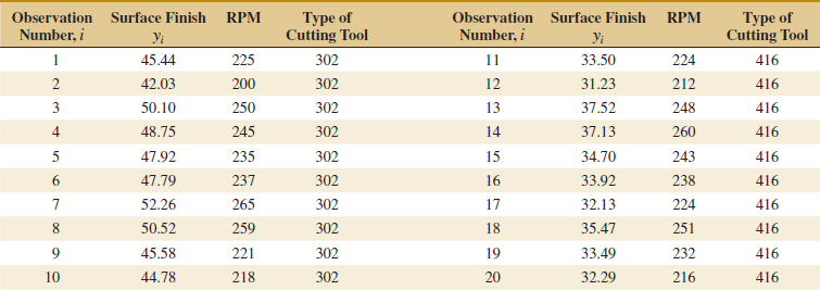
12-6.2 CATEGORICAL REGRESSORS AND INDICATOR VARIABLES
The regression models presented in previous sections have been based on quantitative variables, that is, variables that are measured on a numerical scale. For example, variables such as temperature, pressure, distance, and voltage are quantitative variables. Occasionally, we need to incorporate categorical, or qualitative, variables in a regression model. For example, suppose that one of the variables in a regression model is the operator who is associated with each observation yi. Assume that only two operators are involved. We may wish to assign different levels to the two operators to account for the possibility that each operator may have a different effect on the response.
The usual method of accounting for the different levels of a qualitative variable is to use indicator variables. For example, to introduce the effect of two different operators into a regression model, we could define an indicator variable as follows:
![]()
In general, a qualitative variable with r-levels can be modeled by r − 1 indicator variables, which are assigned the value of either 0 or 1. Thus, if there are three operators, the different levels will be accounted for by the indicator variables defined as follows:
Indicator variables are also referred to as dummy variables. The following example [from Montgomery, Peck, and Vining (2012)] illustrates some of the uses of indicator variables.
Example 12-13 Surface Finish A mechanical engineer is investigating the surface finish of metal parts produced on a lathe and its relationship to the speed (in revolutions per minute) of the lathe. The data are shown in Table 12-11. Note that the data have been collected using two different types of cutting tools. Because the type of cutting tool likely affects the surface finish, we will fit the model
![]()
![]() TABLE • 12-12 Analysis of Variance for Example 12-13
TABLE • 12-12 Analysis of Variance for Example 12-13

where Y is the surface finish, x1 is the lathe speed in revolutions per minute, and x2 is an indicator variable denoting the type of cutting tool used; that is,
![]()
The parameters in this model may be easily interpreted. If x2 = 0, the model becomes
![]()
which is a straight-line model with slope β1 and intercept β0. However, if x2 = 1, the model becomes
![]()
which is a straight-line model with slope β1 and intercept β0 + β2. Thus, the model Y = β0 + β1x + β2x2 + ![]() implies that surface finish is linearly related to lathe speed and that the slope β1 does not depend on the type of cutting tool used. However, the type of cutting tool does affect the intercept, and β2 indicates the change in the intercept associated with a change in tool type from 302 to 416.
implies that surface finish is linearly related to lathe speed and that the slope β1 does not depend on the type of cutting tool used. However, the type of cutting tool does affect the intercept, and β2 indicates the change in the intercept associated with a change in tool type from 302 to 416.
The model matrix X and y vector for this problem are as follows:

![]()
Conclusions: The analysis of variance for this model is shown in Table 12-12. Note that the hypothesis H0: β1 = β2 = 0 (significance of regression) would be rejected at any reasonable level of significance because the P-value is very small. This table also contains the sums of squares
![]()
so a test of the hypothesis H0: β2 = 0 can be made. Because this hypothesis is also rejected, we conclude that tool type has an effect on surface finish.
It is also possible to use indicator variables to investigate whether tool type affects both the slope and intercept. Let the model be
![]()
where x2 is the indicator variable. Now if tool type 302 is used, x2 = 0 and the model is
![]()
If tool type 416 is used, x2 = 1 and the model becomes
![]()
Note that β2 is the change in the intercept and that β3 is the change in slope produced by a change in tool type.
Another method of analyzing these data is to fit separate regression models to the data for each tool type. However, the indicator variable approach has several advantages. First, only one regression model must be fit. Second, by pooling the data on both tool types, more degrees of freedom for error are obtained. Third, tests of both hypotheses on the parameters β2 and β3 are just special cases of the extra sum of squares method.
12-6.3 SELECTION OF VARIABLES AND MODEL BUILDING
An important problem in many applications of regression analysis involves selecting the set of regressor variables to be used in the model. Sometimes previous experience or underlying theoretical considerations can help the analyst specify the set of regressor variables to use in a particular situation. Usually, however, the problem consists of selecting an appropriate set of regressors from a set that quite likely includes all the important variables, but we are sure that not all these candidate regressors are necessary to adequately model the response Y.
In such a situation, we are interested in variable selection; that is, screening the candidate variables to obtain a regression model that contains the “best” subset of regressor variables. We would like the final model to contain enough regressor variables so that in the intended use of the model (prediction, for example), it will perform satisfactorily. On the other hand, to keep model maintenance costs to a minimum and to make the model easy to use, we would like the model to use as few regressor variables as possible. The compromise between these conflicting objectives is often called finding the “best” regression equation. However, in most problems, no single regression model is “best” in terms of the various evaluation criteria that have been proposed. A great deal of judgment and experience with the system being modeled is usually necessary to select an appropriate set of regressor variables for a regression equation.
No single algorithm will always produce a good solution to the variable selection problem. Most of the currently available procedures are search techniques, and to perform satisfactorily, they require interaction with judgment by the analyst. We now briefly discuss some of the more popular variable selection techniques. We assume that there are K candidate regressors, x1, x2,...,xk, and a single response variable y. All models will include an intercept term β0, so the model with all variables included would have K + 1 terms. Furthermore, the functional form of each candidate variable (for example, x1 = 1/x, x2 = ln x, etc.) is assumed to be correct.
All Possible Regressions
This approach requires that the analyst fit all the regression equations involving one candidate variable, all regression equations involving two candidate variables, and so on. Then these equations are evaluated according to some suitable criteria to select the “best” regression model. If there are K candidate regressors, there are 2K total equations to be examined. For example, if K = 4, there are 24 = 16 possible regression equations; if K = 10, there are 210 = 1024 possible regression equations. Hence, the number of equations to be examined increases rapidly as the number of candidate variables increases. However, there are some very efficient computing algorithms for all possible regressions available and they are widely implemented in statistical software, so it is a very practical procedure unless the number of candidate regressors is fairly large. Look for a menu choice such as “Best Subsets” regression.
Several criteria may be used for evaluating and comparing the different regression models obtained. A commonly used criterion is based on the value of R2 or the value of the adjusted R2, ![]() . Basically, the analyst continues to increase the number of variables in the model until the increase in R2 or the adjusted
. Basically, the analyst continues to increase the number of variables in the model until the increase in R2 or the adjusted ![]() is small. Often, we will find that the
is small. Often, we will find that the ![]() will stabilize and actually begin to decrease as the number of variables in the model increases. Usually, the model that maximizes
will stabilize and actually begin to decrease as the number of variables in the model increases. Usually, the model that maximizes ![]() is considered to be a good candidate for the best regression equation. Because we can write
is considered to be a good candidate for the best regression equation. Because we can write ![]() = 1 − {MSE/[SST/(n − 1)]} and SST/(n − 1) is a constant, the model that maximizes the
= 1 − {MSE/[SST/(n − 1)]} and SST/(n − 1) is a constant, the model that maximizes the ![]() value also minimizes the mean square error, so this is a very attractive criterion.
value also minimizes the mean square error, so this is a very attractive criterion.
Another criterion used to evaluate regression models is the Cp statistic, which is a measure of the total mean square error for the regression model. We define the total standardized mean square error for the regression model as
We use the mean square error from the full K + 1 term model as an estimate of σ2; that is, ![]() 2 = MSE(K + 1). Then an estimator of Γp is [see Montgomery, Peck, and Vining (2012) or Myers (1990) for the details]:
2 = MSE(K + 1). Then an estimator of Γp is [see Montgomery, Peck, and Vining (2012) or Myers (1990) for the details]:
Cp Statistic
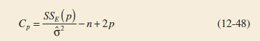
If the P-term model has negligible bias, it can be shown that
![]()
Therefore, the values of Cp for each regression model under consideration should be evaluated relative to p. The regression equations that have negligible bias will have values of Cp that are close to p, and those with significant bias will have values of Cp that are significantly greater than p. We then choose as the “best” regression equation either a model with minimum Cp or a model with a slightly larger Cp, that does not contain as much bias (i.e., Cp ≅ p).
The PRESS statistic can also be used to evaluate competing regression models. PRESS is an acronym for prediction error sum of squares, and it is defined as the sum of the squares of the differences between each observation yi and the corresponding predicted value based on a model fit to the remaining n − 1 points, say ![]() (i). So PRESS provides a measure of how well the model is likely to perform when predicting new data or data that were not used to fit the regression model. The computing formula for PRESS is
(i). So PRESS provides a measure of how well the model is likely to perform when predicting new data or data that were not used to fit the regression model. The computing formula for PRESS is

where ei = yi − ![]() i is the usual residual. Thus PRESS is easy to calculate from the standard least squares regression results. Models that have small values of PRESS are preferred.
i is the usual residual. Thus PRESS is easy to calculate from the standard least squares regression results. Models that have small values of PRESS are preferred.
Example 12-14 Wine Quality Table 12-13 presents data on taste-testing 38 brands of pinot noir wine (the data were first reported in an article by Kwan, Kowalski, and Skogenboe in an article in the Journal Agricultural and Food Chemistry (1979, Vol. 27), and it also appears as one of the default data sets in the Minitab software package). The response variable is y = quality, and we wish to find the “best” regression equation that relates quality to the other five parameters.
Figure 12-12 is the matrix of scatter plots for the wine quality data. We notice that there are some indications of possible linear relationships between quality and the regressors, but there is no obvious visual impression of which regressors would be appropriate. Table 12-14 lists all possible regressions output from the software. In this analysis, we asked the computer software to present the best three equations for each subset size. Note that the computer software reports the values of R2, ![]() , Cp, and S =
, Cp, and S = ![]() for each model. From Table 12-14 we see that the three-variable equation with x2 = aroma, x4 = flavor, and x5 = oakiness produces the minimum Cp equation whereas the four-variable model, which adds x1 = clarity to the previous three regressors, results in maximum
for each model. From Table 12-14 we see that the three-variable equation with x2 = aroma, x4 = flavor, and x5 = oakiness produces the minimum Cp equation whereas the four-variable model, which adds x1 = clarity to the previous three regressors, results in maximum ![]() (or minimum MSE). The three-variable model is
(or minimum MSE). The three-variable model is
![]()
and the four-variable model is
![]()
![]() TABLE • 12-13 Wine Quality Data
TABLE • 12-13 Wine Quality Data


FIGURE 12-12 A matrix of scatter plots from computer software for the wine quality data.
![]() TABLE • 12-14 All Possible Regressions Computer Output for the Wine Quality Data
TABLE • 12-14 All Possible Regressions Computer Output for the Wine Quality Data
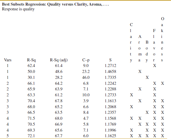
These models should now be evaluated further using residual plots and the other techniques discussed earlier in the chapter to see whether either model is satisfactory with respect to the underlying assumptions and to determine whether one of them is preferable. It turns out that the residual plots do not reveal any major problems with either model. The value of PRESS for the three-variable model is 56.0524, and for the four-variable model, it is 60.3327. Because PRESS is smaller in the model with three regressors, and because it is the model with the smallest number of predictors, it would likely be the preferred choice.
Stepwise Regression
Stepwise regression is probably the most widely used variable selection technique. The procedure iteratively constructs a sequence of regression models by adding or removing variables at each step. The criterion for adding or removing a variable at any step is usually expressed in terms of a partial F-test. Let fin be the value of the F-random variable for adding a variable to the model, and let fout be the value of the F-random variable for removing a variable from the model. We must have fin ≥ fout, and usually fin = fout.
Stepwise regression begins by forming a one-variable model using the regressor variable that has the highest correlation with the response variable Y. This will also be the regressor producing the largest F-statistic. For example, suppose that at this step, x1 is selected. At the second step, the remaining K − 1 candidate variables are examined, and the variable for which the partial F-statistic
![]()
is a maximum is added to the equation provided that fj > fin. In Equation 12-49, MSE(xj, x1) denotes the mean square for error for the model containing both x1 and xj. Suppose that this procedure indicates that x2 should be added to the model. Now the stepwise regression algorithm determines whether the variable x1 added at the first step should be removed. This is done by calculating the F-statistic
![]()
If the calculated value f1 < fout, the variable x1 is removed; otherwise it is retained, and we would attempt to add a regressor to the model containing both x1 and x2.
In general, at each step the set of remaining candidate regressors is examined, and the regressor with the largest partial F-statistic is entered provided that the observed value of f exceeds fin. Then the partial F-statistic for each regressor in the model is calculated, and the regressor with the smallest observed value of F is deleted if the observed f < fout. The procedure continues until no other regressors can be added to or removed from the model.
Stepwise regression is almost always performed using a computer program. The analyst exercises control over the procedure by the choice of fin and fout. Some stepwise regression computer programs require that numerical values be specified for fin and fout. Because the number of degrees of freedom on MSE depends on the number of variables in the model, which changes from step to step, a fixed value of fin and fout causes the type I and type II error rates to vary. Some computer programs allow the analyst to specify the type I error levels for fin and fout. However, the “advertised” significance level is not the true level because the variable selected is the one that maximizes (or minimizes) the partial F-statistic at that stage. Sometimes it is useful to experiment with different values of fin and fout (or different advertised type I error rates) in several different runs to see whether this substantially affects the choice of the final model.
Example 12-15 Wine Quality Stepwise Regression Table 12-15 gives the software stepwise regression output for the wine quality data. The software uses fixed values of a for entering and removing variables. The default level is α = 0.15 for both decisions. The output in Table 12-15 uses the default value. Notice that the variables were entered in the order flavor (step 1), oakiness (step 2), and aroma (step 3) and that no variables were removed. No other variable could be entered, so the algorithm terminated. This is the three-variable model found by all possible regressions that results in a minimum value of Cp.
Forward Selection
The forward selection procedure is a variation of stepwise regression and is based on the principle that regressors should be added to the model one at a time until there are no remaining candidate regressors that produce a significant increase in the regression sum of squares. That is, variables are added one at a time as long as their partial F-value exceeds fin. Forward selection is a simplification of stepwise regression that omits the partial F-test for deleting variables from the model that have been added at previous steps. This is a potential weakness of forward selection; that is, the procedure does not explore the effect that adding a regressor at the current step has on regressor variables added at earlier steps. Notice that if we were to apply forward selection to the wine quality data, we would obtain exactly the same results as we did with stepwise regression in Example 12-15, because stepwise regression terminated without deleting a variable.
Backward Elimination
The backward elimination algorithm begins with all K candidate regressors in the model. Then the regressor with the smallest partial F-statistic is deleted if this F-statistic is insignificant, that is, if f < fout. Next, the model with K − 1 regressors is fit, and the next regressor for potential elimination is found. The algorithm terminates when no further regressor can be deleted.
Table 12-16 shows the computer software package output for backward elimination applied to the wine quality data. The α value for removing a variable is α = 0.10. Notice that this procedure removes body at step 1 and then clarity at step 2, terminating with the three-variable model found previously.
![]() TABLE • 12-15 Stepwise Regression Output for the Wine Quality Data
TABLE • 12-15 Stepwise Regression Output for the Wine Quality Data

![]() TABLE • 12-16 Backward Elimination Output for the Wine Quality Data
TABLE • 12-16 Backward Elimination Output for the Wine Quality Data
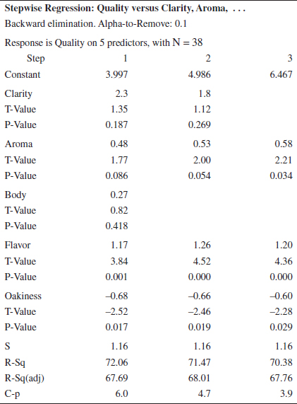
Some Comments on Final Model Selection
We have illustrated several different approaches to the selection of variables in multiple linear regression. The final model obtained from any model-building procedure should be subjected to the usual adequacy checks, such as residual analysis, lack-of-fit testing, and examination of the effects of influential points. The analyst may also consider augmenting the original set of candidate variables with cross-products, polynomial terms, or other transformations of the original variables that might improve the model. A major criticism of variable selection methods such as stepwise regression is that the analyst may conclude that there is one “best” regression equation. Generally, this is not the case because several equally good regression models can often be used. One way to avoid this problem is to use several different model-building techniques and see whether different models result. For example, we have found the same model for the wine quality data using stepwise regression, forward selection, and backward elimination. The same model was also one of the two best found from all possible regressions. The results from variable selection methods frequently do not agree, so this is a good indication that the three-variable model is the best regression equation.
If the number of candidate regressors is not too large, the all-possible regressions method is recommended. We usually recommend using the minimum MSE and Cp evaluation criteria in conjunction with this procedure. The all-possible regressions approach can find the “best” regression equation with respect to these criteria, but stepwise-type methods offer no such assurance. Furthermore, the all-possible regressions procedure is not distorted by dependencies among the regressors as stepwise-type methods are.
12-6.4 MULTICOLLINEARITY
In multiple regression problems, we expect to find dependencies between the response variable Y and the regressors xj. In most regression problems, however, we find that there are also dependencies among the regressor variables xj. In situations in which these dependencies are strong, we say that multicollinearity exists. Multicollinearity can have serious effects on the estimates of the regression coefficients and on the general applicability of the estimated model.
The effects of multicollinearity may be easily demonstrated. The diagonal elements of the matrix C = (X′X)−1 can be written as
![]()
where ![]() is the coefficient of multiple determination resulting from regressing xj on the other k − 1 regressor variables. We can think of
is the coefficient of multiple determination resulting from regressing xj on the other k − 1 regressor variables. We can think of ![]() as a measure of the correlation between xj and the other regressors. Clearly, the stronger the linear dependency of xj on the remaining regressor variables and hence the stronger the multicollinearity, the greater the value of
as a measure of the correlation between xj and the other regressors. Clearly, the stronger the linear dependency of xj on the remaining regressor variables and hence the stronger the multicollinearity, the greater the value of ![]() will be. Recall that V(
will be. Recall that V(![]() j) = σ2Cjj. Therefore, we say that the variance of
j) = σ2Cjj. Therefore, we say that the variance of ![]() j is “inflated” by the quantity (1 −
j is “inflated” by the quantity (1 − ![]() )−1. Consequently, we define the variance inflation factor for βj as
)−1. Consequently, we define the variance inflation factor for βj as
Variance Inflation-Factor (VIF)
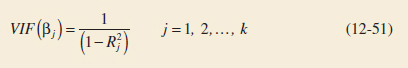
These factors are important measures of the extent to which multicollinearity is present. If the columns of the model matrix X are orthogonal, then the regressors are completely uncorrelated, and the variance inflation factors will all be unity. So, any VIF that exceeds 1 indicates some level of multicollinearity in the data.
Although the estimates of the regression coefficients are very imprecise when multicollinearity is present, the fitted model equation may still be useful. For example, suppose that we wish to predict new observations on the response. If these predictions are interpolations in the original region of the x-space where the multicollinearity is in effect, satisfactory predictions will often be obtained because while individual βj may be poorly estimated, the function ![]() may be estimated quite well. On the other hand, if the prediction of new observations requires extrapolation beyond the original region of the x-space where the data were collected, generally we would expect to obtain poor results. Extrapolation usually requires good estimates of the individual model parameters.
may be estimated quite well. On the other hand, if the prediction of new observations requires extrapolation beyond the original region of the x-space where the data were collected, generally we would expect to obtain poor results. Extrapolation usually requires good estimates of the individual model parameters.
Multicollinearity arises for several reasons. It will occur when the analyst collects data such that a linear constraint holds approximately among the columns of the X matrix. For example, if four regressor variables are the components of a mixture, such a constraint will always exist because the sum of the components is always constant. Usually, these constraints do not hold exactly, and the analyst might not know that they exist.
The presence of multicollinearity can be detected in several ways. Two of the more easily understood of these will be discussed briefly.
- The variance inflation factors, defined in Equation 12-51, are very useful measures of multicollinearity. The larger the variance inflation factor, the more severe the multicollinearity. Some authors have suggested that if any variance inflation factor exceeds 10, multicollinearity is a problem. Other authors consider this value too liberal and suggest that the variance inflation factors should not exceed 4 or 5. Computer software will calculate the variance inflation factors. Table 12-4 presents the computer-generated multiple regression output for the wire bond pull strength data. Because both VIF1 and VIF2 are small, there is no problem with multicollinearity.
- If the F-test for significance of regression is significant but tests on the individual regression coefficients are not significant, multicollinearity may be present.
Several remedial measures have been proposed for solving the problem of multicollinearity. Augmenting the data with new observations specifically designed to break up the approximate linear dependencies that currently exist is often suggested. However, this is sometimes impossible because of economic reasons or because of the physical constraints that relate to the xj. Another possibility is to delete certain variables from the model, but this approach has the disadvantage of discarding the information contained in the deleted variables.
Because multicollinearity primarily affects the stability of the regression coefficients, it would seem that estimating these parameters by some method that is less sensitive to multicollinearity than ordinary least squares would be helpful. Several methods have been suggested. One alternative to ordinary least squares, ridge regression, can be useful in combating multicollinearity. For more details on ridge regression, there are more extensive presentations in Montgomery, Peck, and Vining (2012) and Myers (1990).
Exercises FOR SECTION 12-6
![]() Problem available in WileyPLUS at instructor's discretion.
Problem available in WileyPLUS at instructor's discretion.
![]() Go Tutorial Tutoring problem available in WileyPLUS at instructor's discretion.
Go Tutorial Tutoring problem available in WileyPLUS at instructor's discretion.
![]() 12-84. An article entitled “A Method for Improving the Accuracy of Polynomial Regression Analysis” in the Journal of Quality Technology (1971, pp. 149–155) reported the following data on y = ultimate shear strength of a rubber compound (psi) and x = cure temperature (°F).
12-84. An article entitled “A Method for Improving the Accuracy of Polynomial Regression Analysis” in the Journal of Quality Technology (1971, pp. 149–155) reported the following data on y = ultimate shear strength of a rubber compound (psi) and x = cure temperature (°F).
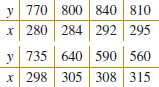
(a) Fit a second-order polynomial to these data.
(b) Test for significance of regression using α = 0.05.
(c) Test the hypothesis that β11 = 0 using α = 0.05.
(d) Compute the residuals from part (a) and use them to evaluate model adequacy.
![]() 12-85. Consider the following data, which result from an experiment to determine the effect of x = test time in hours at a particular temperature on y = change in oil viscosity:
12-85. Consider the following data, which result from an experiment to determine the effect of x = test time in hours at a particular temperature on y = change in oil viscosity:
(a) Fit a second-order polynomial to the data.
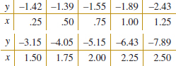
(b) Test for significance of regression using α = 0.05.
(c) Test the hypothesis that β11 = 0 using α = 0.05.
(d) Compute the residuals from part (a) and use them to evaluate model adequacy.
![]()
12-86. The following data were collected during an experiment to determine the change in thrust efficiency (y, in percent) as the divergence angle of a rocket nozzle (x) changes:
(a) Fit a second-order model to the data.
(b) Test for significance of regression and lack of fit using α = 0.05.
(c) Test the hypothesis that β11 = 0, using α = 0.05.
(d) Plot the residuals and comment on model adequacy.
(e) Fit a cubic model, and test for the significance of the cubic term using α = 0.05.
![]()
12-87. An article in the Journal of Pharmaceuticals Sciences (1991, Vol. 80, pp. 971–977) presents data on the observed mole fraction solubility of a solute at a constant temperature and the dispersion, dipolar, and hydrogen-bonding Hansen partial solubility parameters. The data are as shown in the Table E12-13, where y is the negative logarithm of the mole fraction solubility, x1 is the dispersion partial solubility, x2 is the dipolar partial solubility, and x3 is the hydrogen-bonding partial solubility.
(a) Fit the model Y = β0 + β1x1 + β2x2 + β3x3 + β12x1x2 + β13x1x3 + β23x2x3 + ![]() +
+ ![]() .
.
(b) Test for significance of regression using α = 0.05.
(c) Plot the residuals and comment on model adequacy.
(d) Use the extra sum of squares method to test the contribution of the second-order terms using α = 0.05.
![]() TABLE • E12-13 Solubility Data
TABLE • E12-13 Solubility Data

![]()
12-88. Consider the arsenic concentration data in Exercise 12-16.
(a) Discuss how you would model the information about the person's sex.
(b) Fit a regression model to the arsenic in nails using age, drink use, cook use, and the person's sex as the regressors.
(c) Is there evidence that the person's sex affects arsenic in the nails? Why?
![]()
12-89. Consider the gasoline mileage data in Exercise 12-11.
(a) Discuss how you would model the information about the type of transmission in the car.
(b) Fit a regression model to the gasoline mileage using cid, etw and the type of transmission in the car as the regressors.
(c) Is there evidence that the type of transmission (L4, L5, or M6) affects gasoline mileage performance?
![]() 12-90.
12-90. ![]() Consider the surface finish data in Example 12-13. Test the hypothesis that two different regression models (with different slopes and intercepts) are required to adequately model the data. Use indicator variables in answering this question.
Consider the surface finish data in Example 12-13. Test the hypothesis that two different regression models (with different slopes and intercepts) are required to adequately model the data. Use indicator variables in answering this question.
12-91. Consider the X-ray inspection data in Exercise 12-15. Use rads as the response. Build regression models for the data using the following techniques:
(a) All possible regressions.
![]()
(b) Stepwise regression.
(c) Forward selection.
(d) Backward elimination.
(e) Comment on the models obtained. Which model would you prefer? Why?
12-92. ![]() Consider the electric power data in Exercise 12-10. Build regression models for the data using the following techniques:
Consider the electric power data in Exercise 12-10. Build regression models for the data using the following techniques:
(a) All possible regressions. Find the minimum Cp and minimum MSE equations.
![]()
(b) Stepwise regression.
(c) Forward selection.
(d) Backward elimination.
(e) Comment on the models obtained. Which model would you prefer?
12-93. ![]() Consider the regression model fit to the coal and limestone mixture data in Exercise 12-17. Use density as the response. Build regression models for the data using the following techniques:
Consider the regression model fit to the coal and limestone mixture data in Exercise 12-17. Use density as the response. Build regression models for the data using the following techniques:
![]()
(a) All possible regressions.
(b) Stepwise regression.
(c) Forward selection.
(d) Backward elimination.
(e) Comment on the models obtained. Which model would you prefer? Why?
12-94. Consider the wire bond pull strength data in Exercise 12-12. Build regression models for the data using the following methods:
(a) All possible regressions. Find the minimum Cp and minimum MSE equations.
(a) Stepwise regression.
![]()
(b) Forward selection.
(c) Backward elimination.
(d) Comment on the models obtained. Which model would you prefer?
12-95. Consider the gray range modulation data in Exercise 12-19. Use the useful range as the response. Build regression models for the data using the following techniques:
![]()
(a) All possible regressions.
(b) Stepwise regression.
(c) Forward selection.
(d) Backward elimination.
(e) Comment on the models obtained. Which model would you prefer? Why?
12-96. ![]() Consider the nisin extraction data in Exercise 12-18. Build regression models for the data using the following techniques:
Consider the nisin extraction data in Exercise 12-18. Build regression models for the data using the following techniques:
![]()
(a) All possible regressions.
(b) Stepwise regression.
(c) Forward selection.
(d) Backward elimination.
(e) Comment on the models obtained. Which model would you prefer? Why?
12-97. Consider the stack loss data in Exercise 12-20. Build regression models for the data using the following techniques:
(a) All possible regressions.
(b) Stepwise regression.
(c) Forward selection.
(d) Backward elimination.
(e) Comment on the models obtained. Which model would you prefer? Why?
(d) Remove any influential data points and repeat the model building in the previous parts? Does your conclusion in part (e) change?
![]() 12-98.
12-98. ![]() Consider the NHL data in Exercise 12-22. Build regression models for these data with regressors GF through FG using the following methods:
Consider the NHL data in Exercise 12-22. Build regression models for these data with regressors GF through FG using the following methods:
(a) All possible regressions. Find the minimum Cp and minimum MSE equations.
(b) Stepwise regression.
(c) Forward selection.
(d) Backward elimination.
(e) Which model would you prefer?
![]()
12-99. ![]() Use the football data in Exercise 12-21 to build regression models using the following techniques:
Use the football data in Exercise 12-21 to build regression models using the following techniques:
(a) All possible regressions. Find the equations that minimize MSE and that minimize Cp.
(b) Stepwise regression.
(c) Forward selection.
(d) Backward elimination.
(e) Comment on the various models obtained. Which model seems “best,” and why?
![]() 12-100.
12-100. ![]() Consider the arsenic data in Exercise 12-16. Use arsenic in nails as the response and age, drink use, and cook use as the regressors. Build regression models for the data using the following techniques:
Consider the arsenic data in Exercise 12-16. Use arsenic in nails as the response and age, drink use, and cook use as the regressors. Build regression models for the data using the following techniques:
(a) All possible regressions.
(b) Stepwise regression.
(c) Forward selection.
(d) Backward elimination.
(e) Comment on the models obtained. Which model would you prefer? Why?
(f) Now construct an indicator variable and add the person's sex to the list of regressors. Repeat the model building in the previous parts. Does your conclusion in part (e) change?
![]() 12-101. Consider the gas mileage data in Exercise 12-11. Build regression models for the data from the numerical regressors using the following techniques:
12-101. Consider the gas mileage data in Exercise 12-11. Build regression models for the data from the numerical regressors using the following techniques:
(a) All possible regressions.
(b) Stepwise regression.
(c) Forward selection.
(d) Backward elimination.
(e) Comment on the models obtained. Which model would you prefer? Why?
(f) Now construct indicator variable for trns and drv and add these to the list of regressors. Repeat the model building in the previous parts. Does your conclusion in part (e) change?
12-102. ![]() When fitting polynomial regression models, we often subtract
When fitting polynomial regression models, we often subtract ![]() from each
from each ![]() value to produce a “centered” regressor x′ = x −
value to produce a “centered” regressor x′ = x − ![]() . This reduces the effects of dependencies among the model terms and often leads to more accurate estimates of the regression coefficients. Using the data from Exercise 12-84, fit the model Y =
. This reduces the effects of dependencies among the model terms and often leads to more accurate estimates of the regression coefficients. Using the data from Exercise 12-84, fit the model Y = ![]() +
+ ![]() .
.
![]()
(a) Use the results to estimate the coefficients in the uncentered model Y = β0 + β1x + β11x2 + ![]() . Predict y when x = 285°F. Suppose that you use a standardized variable x′ = (x −
. Predict y when x = 285°F. Suppose that you use a standardized variable x′ = (x − ![]() )/sx where sx is the standard deviation of x in constructing a polynomial regression model. Fit the model Y =
)/sx where sx is the standard deviation of x in constructing a polynomial regression model. Fit the model Y = ![]() +
+ ![]() .
.
(b) What value of y do you predict when x = 285°F?
(c) Estimate the regression coefficients in the unstandardized model Y = β0 + β1x + β11x2 + ![]() .
.
(d) What can you say about the relationship between SSE and R2 for the standardized and unstandardized models?
(e) Suppose that y′ = (y − ![]() )/sy is used in the model along with x′. Fit the model and comment on the relationship between SSE and R2 in the standardized model and the unstandardized model.
)/sy is used in the model along with x′. Fit the model and comment on the relationship between SSE and R2 in the standardized model and the unstandardized model.
12-103. ![]() Consider the data in Exercise 12-87. Use all the terms in the full quadratic model as the candidate regressors.
Consider the data in Exercise 12-87. Use all the terms in the full quadratic model as the candidate regressors.
![]()
(a) Use forward selection to identify a model.
(b) Use backward elimination to identify a model.
(c) Compare the two models obtained in parts (a) and (b). Which model would you prefer and why?
12-104. We have used a sample of 30 observations to fit a regression model. The full model has nine regressors, the variance estimate is ![]() 2 = MSE = 100, and R2 = 0.92.
2 = MSE = 100, and R2 = 0.92.
(a) Calculate the F-statistic for testing significance of regression. Using α = 0.05, what would you conclude?
(b) Suppose that we fit another model using only four of the original regressors and that the error sum of squares for this new model is 2200. Find the estimate of σ2 for this new reduced model. Would you conclude that the reduced model is superior to the old one? Why?
(c) Find the value of Cp for the reduced model in part (b). Would you conclude that the reduced model is better than the old model?
12-105. ![]() A sample of 25 observations is used to fit a regression model in seven variables. The estimate of σ2 for this full model is MSE = 10.
A sample of 25 observations is used to fit a regression model in seven variables. The estimate of σ2 for this full model is MSE = 10.
(a) A forward selection algorithm has put three of the original seven regressors in the model. The error sum of squares for the three-variable model is SSE = 300. Based on Cp, would you conclude that the three-variable model has any remaining bias?
(b) After looking at the forward selection model in part (a), suppose you could add one more regressor to the model. This regressor will reduce the error sum of squares to 275. Will the addition of this variable improve the model? Why?
![]() Problem available in WileyPLUS at instructor's discretion.
Problem available in WileyPLUS at instructor's discretion.
![]() Go Tutorial Tutoring problem available in WileyPLUS at instructor's discretion.
Go Tutorial Tutoring problem available in WileyPLUS at instructor's discretion.
12-106. ![]() Consider the following computer output.
Consider the following computer output.

(a) Fill in the missing values. Use bounds for the P-values.
(b) Is the overall model significant at α = 0.05? Is it significant at α = 0.01?
(c) Discuss the contribution of the individual regressors to the model.
12-107. ![]() Consider the following inverse of the model matrix:
Consider the following inverse of the model matrix:

(a) How many variables are in the regression model?
(b) If the estimate of σ2 is 50, what is the estimate of the variance of each regression coefficient?
(c) What is the standard error of the intercept?
![]() 12-108.
12-108. ![]() The data shown in Table E12-14 represent the thrust of a jet-turbine engine (y) and six candidate regressors: x1 = primary speed of rotation, x2 = secondary speed of rotation, x3 = fuel flow rate, x4 = pressure, x5 = exhaust temperature, and x6 = ambient temperature at time of test.
The data shown in Table E12-14 represent the thrust of a jet-turbine engine (y) and six candidate regressors: x1 = primary speed of rotation, x2 = secondary speed of rotation, x3 = fuel flow rate, x4 = pressure, x5 = exhaust temperature, and x6 = ambient temperature at time of test.
(a) Fit a multiple linear regression model using x3 = fuel flow rate, x4 = pressure, and x5 = exhaust temperature as the regressors.
(b) Test for significance of regression using α = 0.01. Find the P-value for this test. What are your conclusions?
(c) Find the t-test statistic for each regressor. Using α = 0.01, explain carefully the conclusion you can draw from these statistics.
(d) Find R2 and the adjusted statistic for this model.
(e) Construct a normal probability plot of the residuals and interpret this graph.
(f) Plot the residuals versus ![]() . Are there any indications of inequality of variance or nonlinearity?
. Are there any indications of inequality of variance or nonlinearity?
(g) Plot the residuals versus x3. Is there any indication of nonlinearity?
(h) Predict the thrust for an engine for which x2 = 28900, x4 = 170, and x5 = 1589.
12-109. Consider the engine thrust data in Exercise 12-108. Refit the model using y* = ln y as the response variable and ![]() = ln3 as the regressor (along with x4 and x5).
= ln3 as the regressor (along with x4 and x5).
![]()
(a) Test for significance of regression using α = 0.01. Find the P-value for this test and state your conclusions.
(b) Use the t-statistic to test H0: βj = 0 versus H1: βj ≠ 0 for each variable in the model. If α = 0.01, what conclusions can you draw?
(c) Plot the residuals versus ![]() * and versus
* and versus ![]() . Comment on these plots. How do they compare with their counterparts obtained in Exercise 12-108 parts (f) and (g)?
. Comment on these plots. How do they compare with their counterparts obtained in Exercise 12-108 parts (f) and (g)?
12-110. ![]() Transient points of an electronic inverter are influenced by many factors. Table E12-15 gives data on the transient point (y, in volts) of PMOS-NMOS inverters and five candidate regressors: x1 = width of the NMOS device, x2 = length of the NMOS device, x3 = width of the PMOS device, x4 = length of the PMOS device, and x5 = temperature (°C).
Transient points of an electronic inverter are influenced by many factors. Table E12-15 gives data on the transient point (y, in volts) of PMOS-NMOS inverters and five candidate regressors: x1 = width of the NMOS device, x2 = length of the NMOS device, x3 = width of the PMOS device, x4 = length of the PMOS device, and x5 = temperature (°C).
![]()
(a) Fit a multiple linear regression model that uses all regressors to these data. Test for significance of regression using α = 0.01. Find the P-value for this test and use it to draw your conclusions.
(b) Test the contribution of each variable to the model using the t-test with α = 0.05. What are your conclusions?
(c) Delete x5 from the model. Test the new model for significance of regression. Also test the relative contribution of each regressor to the new model with the t-test. Using α = 0.05, what are your conclusions?
(d) Notice that the MSE for the model in part (c) is smaller than the MSE for the full model in part (a). Explain why this has occurred.
(e) Calculate the studentized residuals. Do any of these seem unusually large?
(f) Suppose that you learn that the second observation was recorded incorrectly. Delete this observation and refit the model using x1, x2, x3, and x4 as the regressors. Notice that the R2 for this model is considerably higher than the R2 for either of the models fitted previously. Explain why the R2 for this model has increased.
(g) Test the model from part (f) for significance of regression using α = 0.05. Also investigate the contribution of each regressor to the model using the t-test with α = 0.05. What conclusions can you draw?
![]() TABLE • E12-14 Thrust of a Jet-Turbine Engine
TABLE • E12-14 Thrust of a Jet-Turbine Engine

![]() TABLE • E12-15 Transient Point of an Electronic Inverter
TABLE • E12-15 Transient Point of an Electronic Inverter

(h) Plot the residuals from the model in part (f) versus ![]() and versus each of the regressors x1, x2, x3, and x4. Comment on the plots.
and versus each of the regressors x1, x2, x3, and x4. Comment on the plots.
![]() 12-111.
12-111. ![]() Consider the inverter data in Exercise 12-110. Delete observation 2 from the original data. Define new variables as follows: y* = ln y,
Consider the inverter data in Exercise 12-110. Delete observation 2 from the original data. Define new variables as follows: y* = ln y, ![]() , and
, and ![]() .
.
(a) Fit a regression model using these transformed regressors (do not use x5 or x6).
(b) Test the model for significance of regression using α = 0.05. Use the t-test to investigate the contribution of each variable to the model (α = 0.05). What are your conclusions?
(c) Plot the residuals versus ![]() * and versus each of the transformed regressors. Comment on the plots.
* and versus each of the transformed regressors. Comment on the plots.
![]() 12-112.
12-112. ![]() Following are data on y = green liquor (g/l) and x = paper machine speed (feet per minute) from a Kraft paper machine. (The data were read from a graph in an article in the Tappi Journal, March 1986.)
Following are data on y = green liquor (g/l) and x = paper machine speed (feet per minute) from a Kraft paper machine. (The data were read from a graph in an article in the Tappi Journal, March 1986.)
(a) Fit the model Y = β0 + β1x + β2x2 + ![]() using least squares.
using least squares.
(b) Test for significance of regression using α = 0.05. What are your conclusions?
(c) Test the contribution of the quadratic term to the model, over the contribution of the linear term, using an F-statistic. If α = 0.05, what conclusion can you draw?
(d) Plot the residuals from the model in part (a) versus ![]() . Does the plot reveal any inadequacies?
. Does the plot reveal any inadequacies?
(e) Construct a normal probability plot of the residuals. Comment on the normality assumption.
![]()
12-113. Consider the jet engine thrust data in Exercises 12-108 and 12-109. Define the response and regressors as in Exercise 12-109.
(a) Use all possible regressions to select the best regression equation, where the model with the minimum value of MSE is to be selected as “best.”
(b) Repeat part (a) using the Cp criterion to identify the best equation.
(c) Use stepwise regression to select a subset regression model.
(d) Compare the models obtained in parts (a), (b), and (c).
(e) Consider the three-variable regression model. Calculate the variance inflation factors for this model. Would you conclude that multicollinearity is a problem in this model?
![]()
12-114. Consider the electronic inverter data in Exercises 12-110 and 12-111. Define the response and regressors variables as in Exercise 12-111, and delete the second observation in the sample.
(a) Use all possible regressions to find the equation that minimizes Cp.
(b) Use all possible regressions to find the equation that minimizes MSE.
(c) Use stepwise regression to select a subset regression model.
(d) Compare the models you have obtained.
12-115. ![]() A multiple regression model was used to relate y = viscosity of a chemical product to x1 = temperature and x2 = reaction time. The data set consisted of n = 15 observations.
A multiple regression model was used to relate y = viscosity of a chemical product to x1 = temperature and x2 = reaction time. The data set consisted of n = 15 observations.
(a) The estimated regression coefficients were ![]() 0 = 300.00,
0 = 300.00, ![]() 1 = 0.85, and
1 = 0.85, and ![]() 2 = 10.40. Calculate an estimate of mean viscosity when x1 = 100°F and x2 = 2 hours.
2 = 10.40. Calculate an estimate of mean viscosity when x1 = 100°F and x2 = 2 hours.
(b) The sums of squares were SST = 1230.50 and SSE = 120.30. Test for significance of regression using α = 0.05. What conclusion can you draw?
(c) What proportion of total variability in viscosity is accounted for by the variables in this model?
(d) Suppose that another regressor, x3 = stirring rate, is added to the model. The new value of the error sum of squares is SSE = 117.20. Has adding the new variable resulted in a smaller value of MSE? Discuss the significance of this result.
(e) Calculate an F-statistic to assess the contribution of x3 to the model. Using α = 0.05, what conclusions do you reach?
![]()
12-116. Tables E12-16 and E12-17 present statistics for the Major League Baseball 2005 season (The Sports Network).
(a) Consider the batting data. Use model-building methods to predict wins from the other variables. Check that the assumptions for your model are valid.
(b) Repeat part (a) for the pitching data.
(c) Use both the batting and pitching data to build a model to predict wins. What variables are most important? Check that the assumptions for your model are valid.
![]()
12-117. ![]() An article in the Journal of the American Ceramics Society (1992, Vol. 75, pp. 112–116) described a process for immobilizing chemical or nuclear wastes in soil by dissolving the contaminated soil into a glass block. The authors mix CaO and Na2O with soil and model viscosity and electrical conductivity. The electrical conductivity model involves six regressors, and the sample consists of n = 14 observations.
An article in the Journal of the American Ceramics Society (1992, Vol. 75, pp. 112–116) described a process for immobilizing chemical or nuclear wastes in soil by dissolving the contaminated soil into a glass block. The authors mix CaO and Na2O with soil and model viscosity and electrical conductivity. The electrical conductivity model involves six regressors, and the sample consists of n = 14 observations.
![]() TABLE • E12-16 Major League Baseball 2005 Season
TABLE • E12-16 Major League Baseball 2005 Season
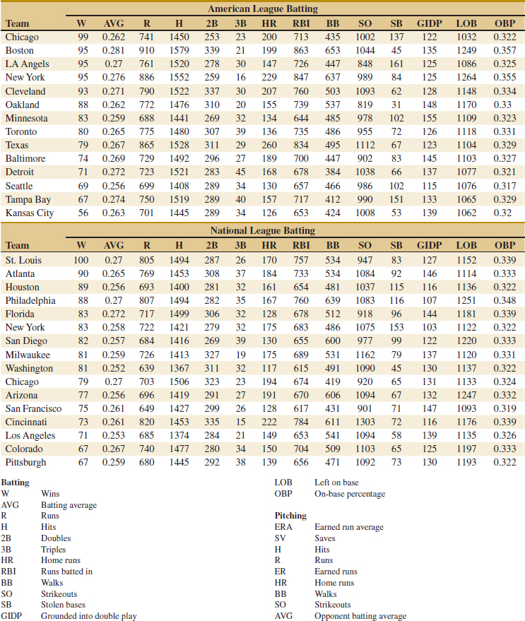
(a) For the six-regressor model, suppose that SST = 0.50 and R2 = 0.94. Find SSE and SSR, and use this information to test for significance of regression with α = 0.05. What are your conclusions?
![]() TABLE • E12-17 Major League Baseball 2005
TABLE • E12-17 Major League Baseball 2005
(b) Suppose that one of the original regressors is deleted from the model, resulting in R2 = 0.92. What can you conclude about the contribution of the variable that was removed? Answer this question by calculating an F-statistic.
(c) Does deletion of the regressor variable in part (b) result in a smaller value of MSE for the five-variable model, in comparison to the original six-variable model? Comment on the significance of your answer.
![]() 12-118. Exercise 12-9 introduced the hospital patient satisfaction survey data. One of the variables in that data set is a categorical variable indicating whether the patient is a medical patient or a surgical patient. Fit a model including this indicator variable to the data using all three of the other regressors. Is there any evidence that the service the patient is on (medical versus surgical) has an impact on the reported satisfaction?
12-118. Exercise 12-9 introduced the hospital patient satisfaction survey data. One of the variables in that data set is a categorical variable indicating whether the patient is a medical patient or a surgical patient. Fit a model including this indicator variable to the data using all three of the other regressors. Is there any evidence that the service the patient is on (medical versus surgical) has an impact on the reported satisfaction?
12-119. Consider the following inverse model matrix.
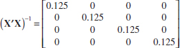
(a) How many regressors are in this model?
(b) What was the sample size?
(c) Notice the special diagonal structure of the matrix. What does that tell you about the columns in the original X matrix?
Mind-Expanding Exercises
12-120. Consider a multiple regression model with k regressors. Show that the test statistic for significance of regression can be written as
![]()
Suppose that n = 20, k = 4, and R2 = 0.90. If α = 0.05, what conclusion would you draw about the relationship between and the four regressors?
12-121. A regression model is used to relate a response to k = 4 regressors with n = 20. What is the smallest value of R2 that will result in a significant regression if α = 0.05? Use the results of the previous exercise. Are you surprised by how small the value of R2 is?
12-122. Show that can express the residuals from a multiple regression model as e = (I − H)y where H = X(X X)−1X′.
12-123. Show that the variance of the ith residual ei in a multiple regression model is σ2(1 − hii) and that the covariance between ei and ej is −σ2hij where the h's are the elements of H = X(X X)−1X′.
12-124. Consider the multiple linear regression model y = Xβ + ![]() . If
. If ![]() denotes the least squares estimator of β, show that
denotes the least squares estimator of β, show that ![]() = β + R
= β + R![]() , where R = (X′X)−1 X′.
, where R = (X′X)−1 X′.
12-125. Constrained Least Squares. Suppose we wish to find the least squares estimator of β in the model y = Xβ + ![]() subject to a set of equality constraints, say, Tβ = c.
subject to a set of equality constraints, say, Tβ = c.
(a) Show that the estimator is
![]()
where ![]() = (X′X)−1 X′y.
= (X′X)−1 X′y.
(b) Discuss situations where this model might be appropriate.
12-126. Piecewise Linear Regression. Suppose that y is piecewise linearly related to x. That is, different linear relationships are appropriate over the intervals −∞ < x ≤ x* and x* < x < ∞.
(a) Show how indicator variables can be used to fit such a piecewise linear regression model, assuming that the point x* is known.
(b) Suppose that at the point x* a discontinuity occurs in the regression function. Show how indicator variables can be used to incorporate the discontinuity into the model.
(c) Suppose that the point x* is not known with certainty and must be estimated. Suggest an approach that could be used to fit the piecewise linear regression model.
Important Terms and Concepts
All possible regressions
Analysis of variance test in multiple regression
Backward elimination
Categorical variables
Confidence interval on the mean response
Cp statistic
Extra sum of squares method
Forward selection
Hat matrix
Hidden extrapolation
Indicator variables
Inference (test and intervals) on individual model parameters
Influential observations
Model parameters and their interpretation in multiple regression
Multicollinearity
Multiple regression model
Outliers
Polynomial regression model
Prediction interval on a future observation
PRESS statistic
Residual analysis and model adequacy checking
R2
Significance of regression
Stepwise regression and related methods
Studentized residuals
Variable selection
Variance inflation factor (VIF)
*There are other methods, such as those described in Montgomery, Peck, and Vining (2012) and Myers (1990), that plot a modified version of the residual, called a partial residual, against each regressor. These partial residual plots are useful in displaying the relationship between the response y and each individual regressor.