

Design of Experiments with Several Factors

Chapter Outline
14-3 Two-Factor Factorial Experiments
14-3.1 Statistical Analysis of the Fixed-Effects Model
14-3.2 Model Adequacy Checking
14-3.3 One Observation per Cell
14-4 General Factorial Experiments
14-5.2 2k Design for k ≥ 3 Factors
14-5.3 Single Replicate of the 2k Design
14-5.4 Addition of Center Points to a 2k Design
14-6 Blocking and Confounding in the 2k Design
14-7 Fractional Replication of the 2k Design
14-7.1 One-Half Fraction of the 2k Design
Carotenoids are fat-soluble pigments that occur naturally in fruits in vegetables and are recommended for healthy diets. A well-known carotenoid is beta-carotene. Astaxanthin is another carotenoid that is a strong antioxidant and commercially produced. An exercise later in this chapter describes an experiment in Biotechnology Progress to promote astaxanthin production. Seven variables were considered important to production: photon flux density and concentrations of nitrogen, phosphorous, magnesium, acetate, ferrous, and NaCl. It was important to study the effects of these factors as well as the effects of combinations on the production. Even with only a high and low setting for each variable, an experiment that uses all possible combinations requires 27 = 128 tests. Such a large experiment has a number of disadvantages, and a question is whether a fraction of the full set of tests can be selected to provide the most important information in many fewer runs. The example used a surprisingly small set of 16 runs (16/128 = 1/8 fraction). The design and analysis of experiments of this type is the focus of this chapter. Such experiments are widely used throughout modern engineering development and scientific studies.
After careful study of this chapter, you should be able to do the following:
- Design and conduct engineering experiments involving several factors using the factorial design approach
- Know how to analyze and interpret main effects and interactions
- Understand how to use the ANOVA to analyze the data from these experiments
- Assess model adequacy with residual plots
- Know how to use the two-level series of factorial designs
- Understand how to run two-level factorial design in blocks
- Design and conduct two-level fractional factorial designs
- Use center points to test for curvature in two-level factorial designs
- Use response surface methodology for process optimization experiments
14-1 Introduction
An experiment is just a test or series of tests. Experiments are performed in all engineering and scientific disciplines and are important parts of the way we learn about how systems and processes work. The validity of the conclusions that are drawn from an experiment depends to a large extent on how the experiment was conducted. Therefore, the design of the experiment plays a major role in the eventual solution to the problem that initially motivated the experiment.
In this chapter, we focus on experiments that include two or more factors that the experimenter thinks may be important. A factorial experiment is a powerful technique for this type of problem. Generally, in a factorial experimental design, experimental trials (or runs) are performed at all combinations of factor levels. For example, if a chemical engineer is interested in investigating the effects of reaction time and reaction temperature on the yield of a process, and if two levels of time (1.0 and 1.5 hours) and two levels of temperature (125 and 150°F) are considered important, a factorial experiment would consist of making experimental runs at each of the four possible combinations of these levels of reaction time and reaction temperature.
Experimental design is an extremely important tool for engineers and scientists who are interested in improving the performance of a manufacturing process. It also has extensive application in the development of new processes and in new product design. We now give some examples.
Process Characterization Experiment
In an article in IEEE Transactions [“Electronics Packaging Manufacturing” (2001, Vol. 24(4), pp. 249–254)], the authors discussed the change to lead-free solder in surface mount technology (SMT). SMT is a process to assemble electronic components to a printed circuit board. Solder paste is printed through a stencil onto the printed circuit board. The stencil-printing machine has squeegees; the paste rolls in front of the squeegee and fills the apertures in the stencil. The squeegee shears off the paste in the apertures as it moves over the stencil. Once the print stroke is completed, the board is separated mechanically from the stencil. Electronic components are placed on the deposits, and the board is heated so that the paste reflows to form the solder joints.
The current SMT soldering process is based on tin–lead solders, and it has been well developed and refined over the years to operate at a competitive cost. The process has several (perhaps many) variables, and all of them are not equally important. The initial list of candidate variables to be included in an experiment is constructed by combining the knowledge and information about the process from all team members. For example, engineers would conduct a brainstorming session and invite manufacturing personnel with SMT experience to participate. SMT has several variables that can be controlled. These include
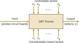
FIGURE 14-1 The flow solder experiment.
(1) squeegee speed, (2) squeegee pressure, (3) squeegee angle, (4) metal or polyurethane squeegee, (5) squeegee vibration, (6) delay time before the squeegee lifts from the stencil, (7) stencil separation speed, (8) print gap, (9) solder paste alloy, (10) paste pretreatment (11) paste particle size, (12) flux type, (13) reflow temperature, (14) reflow time, and so forth.
In addition to these controllable factors, several other factors cannot be easily controlled during routine manufacturing, including
(1) thickness of the printed circuit board, (2) types of components used on the board and aperture width and length, (3) layout of the components on the board, (4) paste density variation, (5) environmental factors, (6) squeegee wear, (7) cleanliness, and so forth.
Sometimes we call the uncontrollable factors noise factors. A schematic representation of the process is shown in Fig. 14-1. In this situation, the engineer wants to characterize the SMT process, that is, to determine the factors (both controllable and uncontrollable) that affect the occurrence of defects on the printed circuit boards. To determine these factors, an experiment can be designed to estimate the magnitude and direction of the factor effects. Sometimes we call such an experiment a screening experiment. The information from this characterization study, or screening experiment, can help determine the critical process variables as well as the direction of adjustment for these factors to reduce the number of defects. It also assists in determining which process variables should be carefully controlled during manufacturing to prevent high defect levels and erratic process performance.
Optimization Experiment
In a characterization experiment, we are interested in determining which factors affect the response. A logical next step is to determine the region in the important factors that leads to an optimum response. For example, if the response is cost, we look for a region of minimum cost. This leads to an optimization experiment.
As an illustration, suppose that the yield of a chemical process is influenced by the operating temperature and the reaction time. We are currently operating the process at 155°F and 1.7 hours of reaction time, and the current process yield is around 75%. See Figure 14-2 for a view of the time–temperature space from above. In this graph, we have connected points of constant yield with lines. These lines are yield contours, and we have shown the contours at 60, 70, 80, 90, and 95% yield. To locate the optimum, we might begin with a factorial experiment such as we describe here, with the two factors, time and temperature, run at two levels each at 10°F and 0.5 hours above and below the current operating conditions. This two-factor factorial design is shown in Fig. 14-2. The average responses observed at the four points in the experiment (145°F, 1.2 hours; 145°F, 2.2 hours; 165°F, 1.2 hours; and 165°F, 2.2 hours) indicate that we should move in the general direction of increased temperature and lower reaction time to increase yield. A few additional runs could be performed in this direction to locate the region of maximum yield.
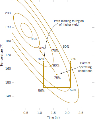
FIGURE 14-2 Contour plot of yield as a function of reaction time and reaction temperature, illustrating an optimization experiment.
Product Design Example
We can also use experimental design in developing new products. For example, suppose that a group of engineers are designing a door hinge for an automobile. The product characteristic is the check effort, or the holding ability, of the latch that prevents the door from swinging closed when the vehicle is parked on a hill. The check mechanism consists of a leaf spring and a roller. When the door is opened, the roller travels through an arc causing the leaf spring to be compressed. To close the door, the spring must be forced aside, creating the check effort. The engineering team thinks that check effort is a function of the following factors:
(1) roller travel distance, (2) spring height from pivot to base, (3) horizontal distance from pivot to spring, (4) free height of the reinforcement spring, (5) free height of the main spring.
The engineers can build a prototype hinge mechanism in which all these factors can be varied over certain ranges. Once appropriate levels for these five factors have been identified, the engineers can design an experiment consisting of various combinations of the factor levels and can test the prototype at these combinations. This produces information concerning which factors are most influential on the latch check effort, and through analysis of this information, the latch design can be improved.
Most of the statistical concepts introduced in Chapter 13 for single-factor experiments can be extended to the factorial experiments of this chapter. The analysis of variance (ANOVA), in particular, continues to be used as a tool for statistical data analysis. We also introduce several graphical methods that are useful in analyzing the data from designed experiments.
14-2 Factorial Experiments
When several factors are of interest in an experiment, a factorial experiment should be used. As noted previously, in these experiments factors are varied together.
By factorial experiment, we mean that in each complete trial or replicate of the experiment, all possible combinations of the levels of the factors are investigated.
Thus, if there are two factors A and B with a levels of factor A and b levels of factor B, each replicate contains all ab treatment combinations.
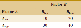
The effect of a factor is defined as the change in response produced by a change in the level of the factor. It is called a main effect because it refers to the primary factors in the study. For example, consider the data in Table 14-1. This is a factorial experiment with two factors, A and B, each at two levels (Alow, Ahigh and Blow, Bhigh). The main effect of factor A is the difference between the average response at the high level of A and the average response at the low level of A, or
![]()
That is, changing factor A from the low level to the high level causes an average response increase of 20 units. Similarly, the main effect of B is
![]()
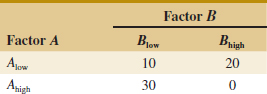
In some experiments, the difference in response between the levels of one factor is not the same at all levels of the other factors. When this occurs, there is an interaction between the factors. For example, consider the data in Table 14-2. At the low level of factor B, the A effect is
![]()
and at the high level of factor B, the A effect is
![]()
Because the effect of A depends on the level chosen for factor B, there is interaction between A and B.
When an interaction is large, the corresponding main effects have very little practical meaning. For example, by using the data in Table 14-2, we find the main effect of A as
![]()
and we would be tempted to conclude that there is no factor A effect. However, when we examined the effects of A at different levels of factor B, we saw that this was not the case. The effect of factor A depends on the levels of factor B. Thus, knowledge of the AB interaction is more useful than knowledge of the main effect. A significant interaction can mask the significance of main effects. Consequently, when interaction is present, the main effects of the factors involved in the interaction may not have much meaning.
It is easy to estimate the interaction effect in factorial experiments such as those illustrated in Tables 14-1 and 14-2. In this type of experiment, when both factors have two levels, the AB interaction effect is the difference in the diagonal averages. This represents one-half the difference between the A effects at the two levels of B. For example, in Table 14-1, we find the AB interaction effect to be
![]() TABLE • 14-1 A Factorial Experiment with Two Factors
TABLE • 14-1 A Factorial Experiment with Two Factors
![]() TABLE • 14-2 A Factorial Experiment with Interaction
TABLE • 14-2 A Factorial Experiment with Interaction
![]()
Thus, there is no interaction between A and B. In Table 14-2, the AB interaction effect is
![]()
As we noted before, the interaction effect in these data is very large.
The concept of interaction can be illustrated graphically in several ways. See Figure 14-3, which plots the data in Table 14-1 against the levels of A for both levels of B. Note that the Blow and Bhigh lines are approximately parallel, indicating that factors A and B do not interact significantly. Figure 14-4 presents a similar plot for the data in Table 14-2. In this graph, the Blow and Bhigh lines are not parallel, indicating the interaction between factors A and B. Such graphical displays are called two-factor interaction plots. They are often useful in presenting the results of experiments, and many computer software programs used for analyzing data from designed experiments construct these graphs automatically.
Figures 14-5 and 14-6 present two other graphical illustrations of the data from Tables 14-1 and 14-2. In Fig. 14-3, we have shown a three-dimensional surface plot of the data from Table 14-1. These data contain no interaction, and the surface plot is a plane lying above the A-B space. The slope of the plane in the A and B directions is proportional to the main effects of factors A and B, respectively. Figure 14-6 is a surface plot of the data from Table 14-2. Notice that the effect of the interaction in these data is to “twist” the plane so that there is curvature in the response function. Factorial experiments are the only way to discover interactions between variables.

FIGURE 14-3 Factorial experiment, no interaction.
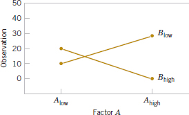
FIGURE 14-4 Factorial experiment, with interaction.
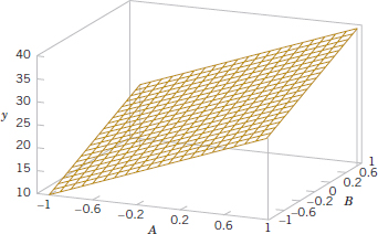
FIGURE 14-5 Three-dimensional surface plot of the data from Table 14-1, showing the main effects of the two factors A and B.
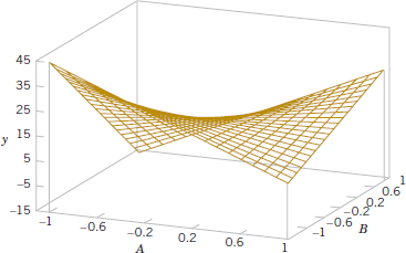
FIGURE 14-6 Three-dimensional surface plot of the data from Table 14-2 showing the effect of the A and B interaction.
An alternative to the factorial design that is (unfortunately) used in practice is to change the factors one at a time rather than to vary them simultaneously. To illustrate this one-factor-at-a-time procedure, suppose that an engineer is interested in finding the values of temperature and pressure that maximize yield in a chemical process. Suppose that we fix temperature at 155°F (the current operating level) and perform five runs at different levels of time, say, 0.5, 1.0, 1.5, 2.0, and 2.5 hours. The results of this series of runs are shown in Fig. 14-7. This figure indicates that maximum yield is achieved at about 1.7 hours of reaction time. To optimize temperature, the engineer then fixes time at 1.7 hours (the apparent optimum) and performs five runs at different temperatures, say, 140, 150, 160, 170, and 180°F. The results of this set of runs are plotted in Fig. 14-8. Maximum yield occurs at about 155°F. Therefore, we would conclude that running the process at 155°F and 1.7 hours is the best set of operating conditions, resulting in yields of around 75%.
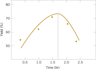
FIGURE 14-7 Yield versus reaction time with temperature constant at 155°F.
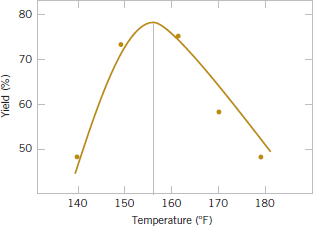
FIGURE 14-8 Yield versus temperature with reaction time constant at 1.7 hours.
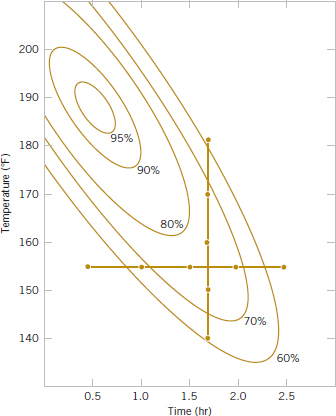
FIGURE 14-9 Optimization experiment using the one-factor-at-a-time method.
Figure 14-9 displays the contour plot of actual process yield as a function of temperature and time with the one-factor-at-a-time experiments superimposed on the contours. Clearly, this one-factor-at-a-time approach has failed dramatically here because the true optimum is at least 20 yield points higher and occurs at much lower reaction times and higher temperatures. The failure to discover the importance of the shorter reaction times is particularly important because this could have significant impact on production volume or capacity, production planning, manufacturing cost, and total productivity.
The one-factor-at-a-time approach has failed here because it cannot detect the interaction between temperature and time. Factorial experiments are the only way to detect interactions. Furthermore, the one-factor-at-a-time method is inefficient. It requires more experimentation than a factorial, and as we have just seen, there is no assurance that it will produce the correct results.
14-3 Two-Factor Factorial Experiments
The simplest type of factorial experiment involves only two factors, say A, and B. There are a levels of factor A and b levels of factor B. This two-factor factorial is shown in Table 14-3. The experiment has n replicates, and each replicate contains all ab treatment combinations. The observation in the ijth cell for the kth replicate is denoted by yijk. In performing the experiment, the abn observations would be run in random order. Thus, like the single-factor experiment studied in Chapter 13, the two-factor factorial is a completely randomized design.
The observations may be described by the linear statistical model
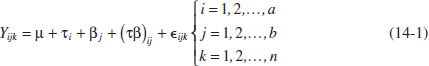
where μ is the overall mean effect, τi is the effect of the ith level of factor A, βj is the effect of the jth level of factor B, (τβ)ij is the effect of the interaction between A and B, and ![]() ijk is a random error component having a normal distribution with mean 0 and variance σ2. We are interested in testing the hypotheses of no main effect for factor A, no main effect for B, and no AB interaction effect. As with the single-factor experiments of Chapter 13, the analysis of variance (ANOVA) is used to test these hypotheses. Because the experiment has two factors, the test procedure is sometimes called the two-way analysis of variance.
ijk is a random error component having a normal distribution with mean 0 and variance σ2. We are interested in testing the hypotheses of no main effect for factor A, no main effect for B, and no AB interaction effect. As with the single-factor experiments of Chapter 13, the analysis of variance (ANOVA) is used to test these hypotheses. Because the experiment has two factors, the test procedure is sometimes called the two-way analysis of variance.
14-3.1 STATISTICAL ANALYSIS OF THE FIXED-EFFECTS MODEL
Suppose that A and B are fixed factors. That is, the a levels of factor A and the b levels of factor B are specifically chosen by the experimenter, and inferences are confined to these levels only. In this model, it is customary to define the effects τi, βj, and (τβ)ij as deviations from the mean, so that ![]() , and
, and ![]() .
.
![]() TABLE • 14-3 Data Arrangement for a Two-Factor Factorial Design
TABLE • 14-3 Data Arrangement for a Two-Factor Factorial Design
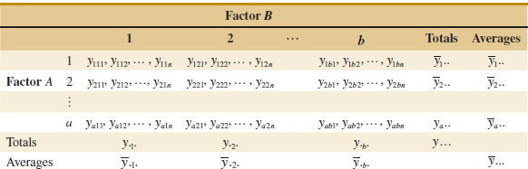
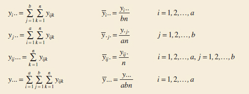
The analysis of variance can be used to test hypotheses about the main factor effects of A and B and the AB interaction. To present the ANOVA, we need some symbols, some of which are illustrated in Table 14-3. Let yi.. denote the total of the observations taken at the ith level of factor A; y·j· denote the total of the observations taken at the jth level of factor B; yij. denote the total of the observations in the ijth cell of Table 14-3; and y... denote the grand total of all the observations. Define ![]() i··,
i··, ![]() ·j·,
·j·, ![]() ij·, and
ij·, and ![]() ... as the corresponding row, column, cell, and grand averages. That is,
... as the corresponding row, column, cell, and grand averages. That is,
Notation for Totals and Means
The hypotheses that we will test are as follows:
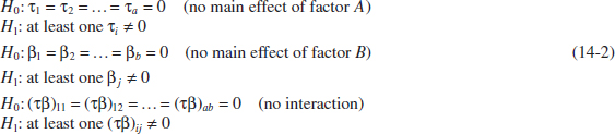
As before, the ANOVA tests these hypotheses by decomposing the total variability in the data into component parts and then comparing the various elements in this decomposition. Total variability is measured by the total sum of squares of the observations
![]()
and the definition of the sum of squares decomposition follows.
ANOVA Sum of Squares Identity: Two Factors
The sum of squares identity for a two-factor ANOVA is
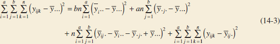
or symbolically,
![]()
Equations 14-3 and 14-4 state that the total sum of squares SST is partitioned into a sum of squares for the row factor A (SSA), a sum of squares for the column factor B(SSB), a sum of squares for the interaction between A and B(SSAB), and an error sum of squares (SSE). There are abn − 1 total degrees of freedom. The main effects A and B have a − 1 and b − 1 degrees of freedom, and the interaction effect AB has (a − 1)(b − 1) degrees of freedom. Within each of the ab cells in Table 14-3, there are n − 1 degrees of freedom between the n replicates, and observations in the same cell can differ only because of random error. Therefore, there are ab(n − 1) degrees of freedom for error, so the degrees of freedom are partitioned according to
![]()
If we divide each of the sum of squares on the right-hand side of Equation 14-4 by the corresponding number of degrees of freedom, we obtain the mean squares for A, B, the interaction, and error:
![]()
Assuming that factors A and B are fixed factors, it is not difficult to show that the expected values of these mean squares are
Expected Values of Mean Squares: Two Factors
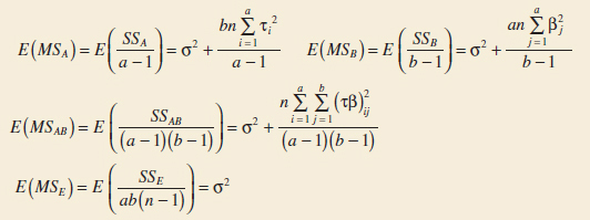
From examining these expected mean squares, it is clear that if the null hypotheses about main effects H0: τi = 0, H0: βj = 0, and the interaction hypothesis H0: (τβ)ij = 0 are all true, all four mean squares are unbiased estimates of σ2.
To test that the row factor effects are all equal to zero (H0: τi = 0), we would use the ratio
F Test for Factor A

which has an F distribution with a − 1 and ab(n − 1) degrees of freedom if H0: τi = 0 is true. This null hypothesis is rejected at the α level of significance if f0 > fα,a−1,ab(n−1). Similarly, to test the hypothesis that all the column factor effects are equal to 0(H0: βj = 0), we would use the ratio
F Test for Factor A

which has an F distribution with b − 1 and ab(n − 1) degrees of freedom if H0: βj = 0 is true. This null hypothesis is rejected at the α level of significance if f0 > fα,b−1,ab(n−1). Finally, to test the hypothesis H0: (τβ)ij = 0, which is the hypothesis that all interaction effects are 0, we use the ratio
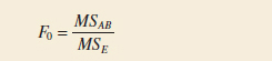
which has an F distribution with (a − 1)(b − 1) and ab(n − 1) degrees of freedom if the null hypothesis H0: (τβ)ij = 0. This hypothesis is rejected at the a level of significance if f0 > fα, (a−1)(b−1), ab(n−1).
It is usually best to conduct the test for interaction first and then to evaluate the main effects. If interaction is not significant, interpretation of the tests on the main effects is straightforward. However, as noted in Section 14-3, when interaction is significant, the main effects of the factors involved in the interaction may not have much practical interpretative value. Knowledge of the interaction is usually more important than knowledge about the main effects.
Computational formulas for the sums of squares are easily obtained.
Computing Formulas for ANOVA: Two Factors
Computing formulas for the sums of squares in a two-factor analysis of variance:
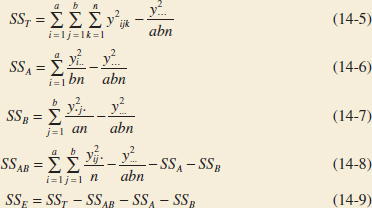
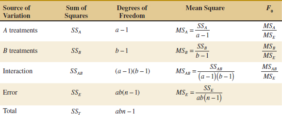
The computations are usually displayed in an ANOVA table, such as Table 14-4.
![]() TABLE • 14-4 ANOVA Table for a Two-Factor Factorial, Fixed-Effects Model
TABLE • 14-4 ANOVA Table for a Two-Factor Factorial, Fixed-Effects Model
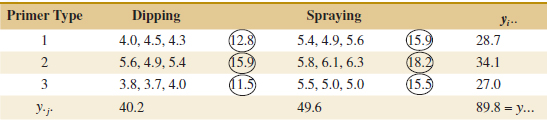
Example 14-1 Aircraft Primer Paint Aircraft primer paints are applied to aluminum surfaces by two methods: dipping and spraying. The purpose of using the primer is to improve paint adhesion, and some parts can be primed using either application method. The process engineering group responsible for this operation is interested in learning whether three different primers differ in their adhesion properties. A factorial experiment was performed to investigate the effect of paint primer type and application method on paint adhesion. For each combination of primer type and application method, three specimens were painted, then a finish paint was applied, and the adhesion force was measured. The data from the experiment are shown in Table 14-5. The circled numbers in the cells are the cell totals yij·· The sums of squares required to perform the ANOVA are computed as follows:
![]() TABLE • 14-5 Adhesion Force Data for Example 14-1
TABLE • 14-5 Adhesion Force Data for Example 14-1
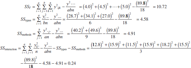
and
![]()
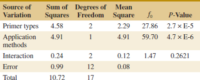
The ANOVA is summarized in Table 14-6. The experimenter has decided to use α = 0.05. Because f0.05,2,12 = 3.89 and f0.05,1,12 = 4.75, we conclude that the main effects of primer type and application method affect adhesion force. Furthermore, because 1.5 < f0.05,2,12, there is no indication of interaction between these factors. The last column of Table 14-6 shows the P-value for each F-ratio. Notice that the P-values for the two test statistics for the main effects are considerably less than 0.05, and the P-value for the test statistic for the interaction is more than 0.05.
Practical Interpretation: See a graph of the cell adhesion force averages {![]() ij·} versus levels of primer type for each application method in Fig. 14-10. The no-interaction conclusion is obvious in this graph, because the two lines are nearly parallel. Furthermore, because a large response indicates greater adhesion force, we conclude that spraying is the best application method and that primer type 2 is most effective.
ij·} versus levels of primer type for each application method in Fig. 14-10. The no-interaction conclusion is obvious in this graph, because the two lines are nearly parallel. Furthermore, because a large response indicates greater adhesion force, we conclude that spraying is the best application method and that primer type 2 is most effective.
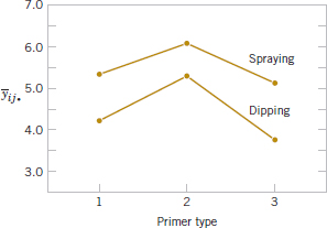
FIGURE 14-10 Graph of average adhesion force versus primer types for both application methods.
![]() TABLE • 14-6 ANOVA for Aircraft Primer Paint Experiment in Example 14-1
TABLE • 14-6 ANOVA for Aircraft Primer Paint Experiment in Example 14-1
Tests on Individual Means
When both factors are fixed, comparisons between the individual means of either factor may be made using any multiple comparison technique such as Fisher's LSD method (described in Chapter 13). When there is no interaction, these comparisons may be made using either the row averages ![]() i·· or the column averages
i·· or the column averages ![]() ·j·. However, when interaction is significant, comparisons between the means of one factor (say, A) may be obscured by the AB interaction. In this case, we could apply a procedure such as Fisher's LSD method to the means of factor A, with factor B set at a particular level.
·j·. However, when interaction is significant, comparisons between the means of one factor (say, A) may be obscured by the AB interaction. In this case, we could apply a procedure such as Fisher's LSD method to the means of factor A, with factor B set at a particular level.
Computer Output
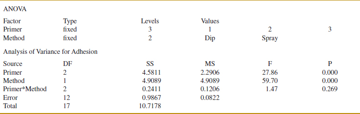
Table 14-7 shows some computer output from the analysis of variance procedure for the aircraft primer paint experiment in Example 14-1. The upper portion of the table gives factor name and level information, and the lower portion presents the analysis of variance for the adhesion force response. The results are identical to the manual calculations displayed in Table 14-6 apart from rounding.
14-3.2 MODEL ADEQUACY CHECKING
Just as in the single-factor experiments discussed in Chapter 13, the residuals from a factorial experiment play an important role in assessing model adequacy. The residuals from a two-factor factorial are
![]()
That is, the residuals are just the difference between the observations and the corresponding cell averages.
Refer to Table 14-8 for the residuals for the aircraft primer paint data in Example 14-1. See Fig. 14-11 for the normal probability plot of these residuals. This plot has tails that do not fall exactly along a straight line passing through the center of the plot, indicating some potential problems with the normality assumption, but the deviation from normality does not appear severe. Figures 14-12 and 14-13 plot the residuals versus the levels of primer types and application methods, respectively. There is some indication that primer type 3 results in slightly lower variability in adhesion force than the other two primers. The graph of residuals versus fitted values in Fig. 14-14 does not reveal any unusual or diagnostic pattern.
![]() TABLE • 14-7 Analysis of Variance from Computer Software for the Aircraft Primer Paint Experiment in Example 14-1
TABLE • 14-7 Analysis of Variance from Computer Software for the Aircraft Primer Paint Experiment in Example 14-1
![]() TABLE • 14-8 Residuals for the Aircraft Primer Paint Experiment in Example 14-1
TABLE • 14-8 Residuals for the Aircraft Primer Paint Experiment in Example 14-1
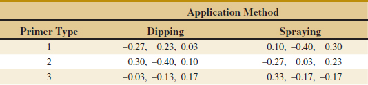
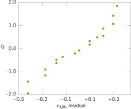
FIGURE 14-11 Normal probability plot of the residuals from the aircraft primer paint experiment in Example 14-1.
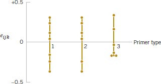
FIGURE 14-12 Plot of residuals from the aircraft primer paint experiment versus primer type.
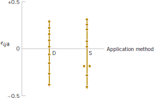
FIGURE 14-13 Plot of residuals from the aircraft primer paint experiment versus application method.
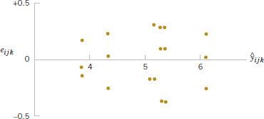
FIGURE 14-14 Plot of residuals from the aircraft primer paint experiment versus predicted values ![]() ijk.
ijk.
14-3.3 ONE OBSERVATION PER CELL
In some cases involving a two-factor factorial experiment, we may have only one replicate—that is, only one observation per cell. In this situation, there are exactly as many parameters in the analysis of variance model as observations, and the error degrees of freedom are zero. Thus, we cannot test hypotheses about the main effects and interactions unless we make some additional assumptions. One possible assumption is to assume that the interaction effect is negligible and use the interaction mean square as an error mean square. Thus, the analysis is equivalent to the analysis used in the randomized block design. This no-interaction assumption can be dangerous, and the experimenter should carefully examine the data and the residuals for indications of whether or not interaction is present. For more details, see Montgomery (2012).
![]() Problem available in WileyPLUS at instructor's discretion.
Problem available in WileyPLUS at instructor's discretion.
![]() Go Tutorial Tutoring problem available in WileyPLUS at instructor's discretion.
Go Tutorial Tutoring problem available in WileyPLUS at instructor's discretion.
![]() 14-1.
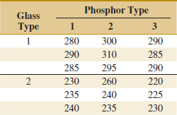
14-1. ![]() An article in Industrial Quality Control (1956, pp. 5–8) describes an experiment to investigate the effect of two factors (glass type and phosphor type) on the brightness of a television tube. The response variable measured is the current (in microamps) necessary to obtain a specified brightness level. The data are shown in the following table:
An article in Industrial Quality Control (1956, pp. 5–8) describes an experiment to investigate the effect of two factors (glass type and phosphor type) on the brightness of a television tube. The response variable measured is the current (in microamps) necessary to obtain a specified brightness level. The data are shown in the following table:
(a) State the hypotheses of interest in this experiment.
(b) Test the hypotheses in part (a) and draw conclusions using the analysis of variance with α = 0.05.
(c) Analyze the residuals from this experiment.
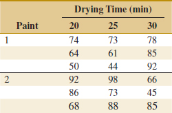
![]() 14-2. An engineer suspects that the surface finish of metal parts is influenced by the type of paint used and the drying time. He selected three drying times—20, 25, and 30 minutes—and used two types of paint. Three parts are tested with each combination of paint type and drying time. The data are as follows:
14-2. An engineer suspects that the surface finish of metal parts is influenced by the type of paint used and the drying time. He selected three drying times—20, 25, and 30 minutes—and used two types of paint. Three parts are tested with each combination of paint type and drying time. The data are as follows:
(a) State the hypotheses of interest in this experiment.
(b) Test the hypotheses in part (a) and draw conclusions using the analysis of variance with α = 0.05.
(c) Analyze the residuals from this experiment.
![]() 14-3.
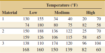
14-3. ![]() In the book Design and Analysis of Experiments, 8th edition (2012, John Wiley & Sons), the results of an experiment involving a storage battery used in the launching mechanism of a shoulder-fired ground-to-air missile were presented. Three material types can be used to make the battery plates. The objective is to design a battery that is relatively unaffected by the ambient temperature. The output response from the battery is effective life in hours. Three temperature levels are selected, and a factorial experiment with four replicates is run. The data are as follows:
In the book Design and Analysis of Experiments, 8th edition (2012, John Wiley & Sons), the results of an experiment involving a storage battery used in the launching mechanism of a shoulder-fired ground-to-air missile were presented. Three material types can be used to make the battery plates. The objective is to design a battery that is relatively unaffected by the ambient temperature. The output response from the battery is effective life in hours. Three temperature levels are selected, and a factorial experiment with four replicates is run. The data are as follows:
(a) Test the appropriate hypotheses and draw conclusions using the analysis of variance with α = 0.05.
(b) Graphically analyze the interaction.
(c) Analyze the residuals from this experiment.
![]()
14-4. An experiment was conducted to determine whether either firing temperature or furnace position affects the baked density of a carbon anode. The data are as follows:
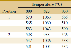
(a) State the hypotheses of interest.
(b) Test the hypotheses in part (a) using the analysis of variance with α = 0.05. What are your conclusions?
(c) Analyze the residuals from this experiment.
(d) Using Fisher's LSD method, investigate the differences between the mean baked anode density at the three different levels of temperature. Use α = 0.05.
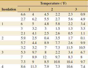
14-5. An article in Technometrics [“Exact Analysis of Means with Unequal Variances” (2002, Vol. 44, pp. 152–160)] described the technique of the analysis of means (ANOM) and presented the results of an experiment on insulation. Four insulation types were tested at three different temperatures. The data are as follows:
(a) Write a model for this experiment.
(b) Test the appropriate hypotheses and draw conclusions using the analysis of variance with α = 0.05
(c) Graphically analyze the interaction.
(d) Analyze the residuals from the experiment.
(e) Use Fisher's LSD method to investigate the differences between mean effects of insulation type. Use α = 0.05.
![]() 14-6. Johnson and Leone (Statistics and Experimental Design in Engineering and the Physical Sciences, John Wiley, 1977) described an experiment conducted to investigate warping of copper plates. The two factors studied were temperature and the copper content of the plates. The response variable is the amount of warping. The data are as follows:
14-6. Johnson and Leone (Statistics and Experimental Design in Engineering and the Physical Sciences, John Wiley, 1977) described an experiment conducted to investigate warping of copper plates. The two factors studied were temperature and the copper content of the plates. The response variable is the amount of warping. The data are as follows:
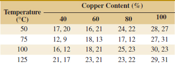
(a) Is there any indication that either factor affects the amount of warping? Is there any interaction between the factors? Use α = 0.05.
(b) Analyze the residuals from this experiment.
(c) Plot the average warping at each level of copper content and compare the levels using Fisher's LSD method. Describe the differences in the effects of the different levels of copper content on warping. If low warping is desirable, what level of copper content would you specify?
(d) Suppose that temperature cannot be easily controlled in the environment in which the copper plates are to be used. Does this change your answer for part (c)?
![]() 14-7.
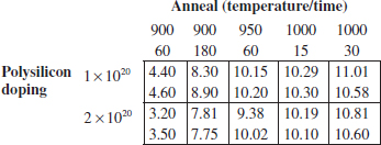
14-7. ![]() An article in the IEEE Transactions on Electron Devices (November 1986, p. 1754) described a study on the effects of two variables—polysilicon doping and anneal conditions (time and temperature)—on the base current of a bipolar transistor. The data from this experiment follow.
An article in the IEEE Transactions on Electron Devices (November 1986, p. 1754) described a study on the effects of two variables—polysilicon doping and anneal conditions (time and temperature)—on the base current of a bipolar transistor. The data from this experiment follow.
(a) Is there any evidence to support the claim that either polysilicon doping level or anneal conditions affect base current? Do these variables interact? Use α = 0.05.
(b) Graphically analyze the interaction.
(c) Analyze the residuals from this experiment.
(d) Use Fisher's LSD method to isolate the effects of anneal conditions on base current, with α = 0.05.
![]()
14-8. An article in the Journal of Testing and Evaluation (1988, Vol. 16, pp. 508–515) investigated the effects of cyclic loading frequency and environment conditions on fatigue crack growth at a constant 22 MPa stress for a particular material. The data follow. The response variable is fatigue crack growth rate.
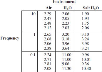
(a) Is there indication that either factor affects crack growth rate? Is there any indication of interaction? Use α = 0.05.
(b) Analyze the residuals from this experiment.
(c) Repeat the analysis in part (a) using ln(y) as the response. Analyze the residuals from this new response variable and comment on the results.
![]()
14-9. Consider a two-factor factorial experiment. Develop a formula for finding a 100(1 − α)% confidence interval on the difference between any two means for either a row or column factor. Apply this formula to find a 95% CI on the difference in mean warping at the levels of copper content 60 and 80% in Exercise 14-6.
![]() TABLE • E14-1 Data for Antifungal Activities
TABLE • E14-1 Data for Antifungal Activities
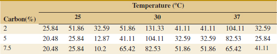
![]() 14-10. An article in Journal of Chemical Technology and Biotechnology [“A Study of Antifungal Antibiotic Production by Thermomonospora sp MTCC 3340 Using Full Factorial Design” (2003, Vol. 78, pp. 605–610)] considered the effects of several factors on antifungal activities. The antifungal yield was expressed as Nystatin international units per cm3. The results from carbon source concentration (glucose) and incubation temperature factors follow. See Table E14-1.
14-10. An article in Journal of Chemical Technology and Biotechnology [“A Study of Antifungal Antibiotic Production by Thermomonospora sp MTCC 3340 Using Full Factorial Design” (2003, Vol. 78, pp. 605–610)] considered the effects of several factors on antifungal activities. The antifungal yield was expressed as Nystatin international units per cm3. The results from carbon source concentration (glucose) and incubation temperature factors follow. See Table E14-1.
(a) State the hypotheses of interest.
(b) Test your hypotheses with α = 0.5.
(c) Analyze the residuals and plot the residuals versus the predicted yield.
(d) Using Fisher's LSD method, compare the means of antifungal activity for the different carbon source concentrations.
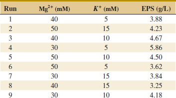
![]() 14-11. An article in Bioresource Technology [“Quantitative Response of Cell Growth and Tuber Polysaccharides Biosynthesis by Medicinal Mushroom Chinese Truffle Tuber Sinense to Metal Ion in Culture Medium” (2008, Vol. 99(16), pp. 7606–7615)] described an experiment to investigate the effect of metal ion concentration to the production of extracellular polysaccharides (EPS). It is suspected that Mg2+ and K+ (in millimolars) are related to EPS. The data from a full factorial design follow.
14-11. An article in Bioresource Technology [“Quantitative Response of Cell Growth and Tuber Polysaccharides Biosynthesis by Medicinal Mushroom Chinese Truffle Tuber Sinense to Metal Ion in Culture Medium” (2008, Vol. 99(16), pp. 7606–7615)] described an experiment to investigate the effect of metal ion concentration to the production of extracellular polysaccharides (EPS). It is suspected that Mg2+ and K+ (in millimolars) are related to EPS. The data from a full factorial design follow.
(a) State the hypotheses of interest.
(b) Test the hypotheses with α = 0.5.
(c) Analyze the residuals and plot residuals versus the predicted production.
14-4 General Factorial Experiments
Many experiments involve more than two factors. In this section, we introduce the case in which there are a levels of factor A, b levels of factor B, c levels of factor C, and so on, arranged in a factorial experiment. In general, there are a × b × c ··· × n total observations if there are n replicates of the complete experiment.
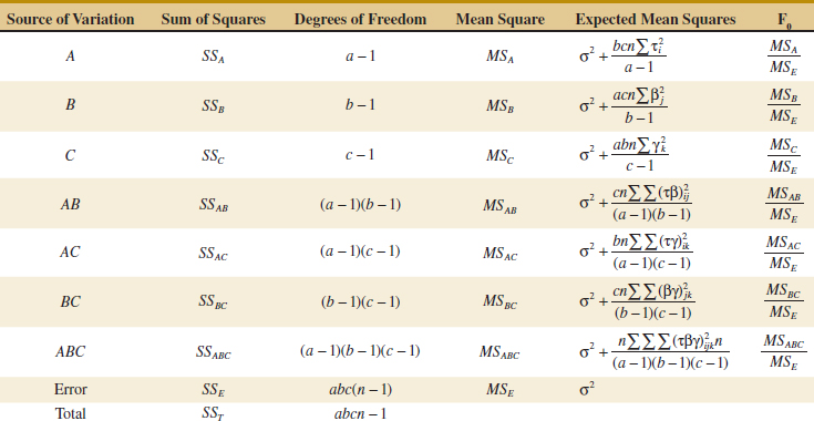
For example, consider the three-factor-factorial experiment, with underlying model
Notice that the model contains three main effects, three two-factor interactions, a three-factor interaction, and an error term. Assuming that A, B, and C are fixed factors, the analysis of variance is shown in Table 14-9. Note that there must be at least two replicates (n ≥ 2) to compute an error sum of squares. The F-test on main effects and interactions follows directly from the expected mean squares. These ratios follow F-distributions under the respective null hypotheses.
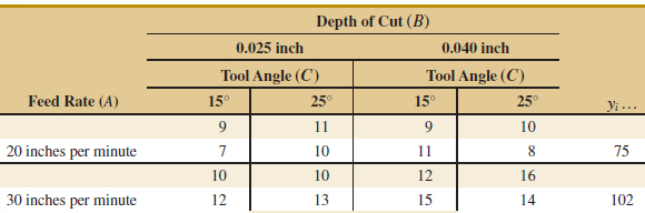
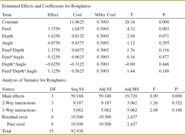
Example 14-2 Surface Roughness A mechanical engineer is studying the surface roughness of a part produced in a metal-cutting operation. Three factors, feed rate (A), depth of cut (B), and tool angle (C), are of interest. All three factors have been assigned two levels, and two replicates of a factorial design are run. The coded data are in Table 14-10.
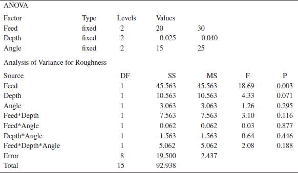
The ANOVA is summarized in Table 14-11. Because manual ANOVA computations are tedious for three-factor experiments, we have used computer software for the solution of this problem. The F-ratios for all three main effects and the interactions are formed by dividing the mean square for the effect of interest by the error mean square. Because the experimenter has selected α = 0.05, the critical value for each of these F-ratios is f0.05,1,8 = 5.32. Alternately, we could use the P-value approach. The P-values for all the test statistics are shown in the last column of Table 14-11. Inspection of these P-values is revealing. There is a strong main effect of feed rate, because the F-ratio is well into the critical region. However, there is some indication of an effect due to the depth of cut because P = 0.0710 is not much greater than α = 0.05. The next largest effect is the AB or feed rate × depth of cut interaction. Most likely, both feed rate and depth of cut are important process variables.
Practical Interpretation: Further experiments could study the important factors in more detail to improve the surface roughness.
Obviously, factorial experiments with three or more factors can require many runs, particularly if some of the factors have several (more than two) levels. This point of view leads us to the class of factorial designs considered in Section 14-5 with all factors at two levels. These designs are easy to set up and analyze, and they may be used as the basis of many other useful experimental designs.
![]() TABLE • 14-9 Analysis of Variance Table for the Three-Factor Fixed Effects Model
TABLE • 14-9 Analysis of Variance Table for the Three-Factor Fixed Effects Model
![]() TABLE • 14-10 Coded Surface Roughness Data for Example 14-2
TABLE • 14-10 Coded Surface Roughness Data for Example 14-2
![]() TABLE • 14-11 ANOVA for Example 14-2
TABLE • 14-11 ANOVA for Example 14-2
Exercises FOR SECTION 14-4
![]() Problem available in WileyPLUS at instructor's discretion
Problem available in WileyPLUS at instructor's discretion
![]() Go Tutorial Tutoring problem available in WileyPLUS at instructor's discretion.
Go Tutorial Tutoring problem available in WileyPLUS at instructor's discretion.
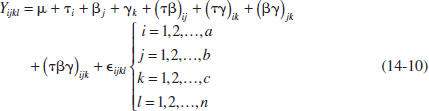
![]() 14-12. The quality control department of a fabric finishing plant is studying the effects of several factors on dyeing for a blended cotton/synthetic cloth used to manufacture shirts. Three operators, three cycle times, and two temperatures were selected, and three small specimens of cloth were dyed under each set of conditions. The finished cloth was compared to a standard, and a numerical score was assigned. The results are shown in the following table.
14-12. The quality control department of a fabric finishing plant is studying the effects of several factors on dyeing for a blended cotton/synthetic cloth used to manufacture shirts. Three operators, three cycle times, and two temperatures were selected, and three small specimens of cloth were dyed under each set of conditions. The finished cloth was compared to a standard, and a numerical score was assigned. The results are shown in the following table.
(a) State and test the appropriate hypotheses using the analysis of variance with α = 0.05.
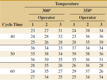
(b) The residuals may be obtained from eijkl = yijkl − ![]() ijk·. Graphically analyze the residuals from this experiment.
ijk·. Graphically analyze the residuals from this experiment.
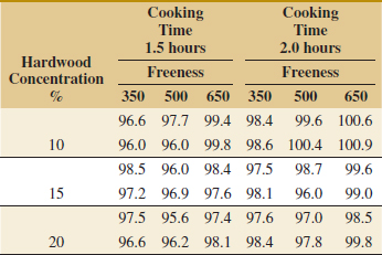
14-13. ![]() The percentage of hardwood concentration in raw pulp, the freeness, and the cooking time of the pulp are being investigated for their effects on the strength of paper. The data from a three-factor factorial experiment are shown in the following table.
The percentage of hardwood concentration in raw pulp, the freeness, and the cooking time of the pulp are being investigated for their effects on the strength of paper. The data from a three-factor factorial experiment are shown in the following table.
![]()
(a) Analyze the data using the analysis of variance assuming that all factors are fixed. Use α = 0.05.
(b) Compute approximate P-values for the F-ratios in part (a).
(c) The residuals are found from eijkl = yijkl − ![]() ijk·. Graphically analyze the residuals from this experiment.
ijk·. Graphically analyze the residuals from this experiment.
14-5 2k Factorial Designs
Factorial designs are frequently used in experiments involving several factors where it is necessary to study the joint effect of the factors on a response. However, several special cases of the general factorial design are important because they are widely employed in research work and because they form the basis of other designs of considerable practical value.
The most important of these special cases is that of k factors, each at only two levels. These levels may be quantitative, such as two values of temperature, pressure, or time; or they may be qualitative, such as two machines, two operators, the “high” and “low” levels of a factor, or perhaps the presence and absence of a factor. A complete replicate of such a design requires 2 × 2 × ... × 2 = 2k observations and is called a 2k factorial design.
The 2k design is particularly useful in the early stages of experimental work when many factors are likely to be investigated. It provides the smallest number of runs for which k factors can be studied in a complete factorial design. Because each factor has only two levels, we must assume that the response is approximately linear over the range of the factor levels chosen.
14-5.1 22 DESIGN
The simplest type of 2k design is the 22—that is, two factors A and B, each at two levels. We usually think of these levels as the factor's low and high levels. The 22 design is shown in Fig. 14-15. Note that the design can be represented geometrically as a square with the 22 = 4 runs, or treatment combinations, forming the corners of the square. In the 22 design, it is customary to denote the low and high levels of the factors A and B by the signs − and +, respectively. This is sometimes called the geometric notation for the design.
A special notation is used to label the treatment combinations. In general, a treatment combination is represented by a series of lowercase letters. If a letter is present, the corresponding factor is run at the high level in that treatment combination; if it is absent, the factor is run at its low level. For example, treatment combination a indicates that factor A is at the high level and factor B is at the low level. The treatment combination with both factors at the low level is represented by (1). This notation is used throughout the 2k design series. For example, the treatment combination in a 24 with A and C at the high level and B and D at the low level is denoted by ac.
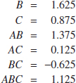
The effects of interest in the 22 design are the main effects A and B and the two-factor interaction AB. Let the symbols (1), a, b, and ab also represent the totals of all n observations taken at these design points. It is easy to estimate the effects of these factors. To estimate the main effect of A, we would average the observations on the right side of the square in Fig. 14-15 where A is at the high level, and subtract from this the average of the observations on the left side of the square where A is at the low level, or
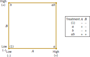
FIGURE 14-15 The 22 factorial design.
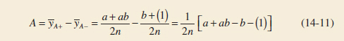
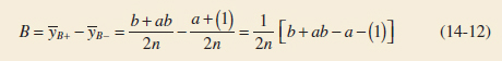
Similarly, the main effect of B is found by averaging the observations on the top of the square, where B is at the high level, and subtracting the average of the observations on the bottom of the square, where B is at the low level:
Main Effect of Factor B:22 Design
Finally, the AB interaction is estimated by taking the difference in the diagonal averages in Fig. 14-15, or
Interaction Effect AB:22 Design
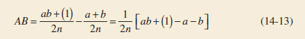
The quantities in brackets in Equations 14-11, 14-12, and 14-13 are called contrasts. For example, the A contrast is
![]()
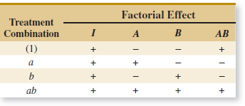
In these equations, the contrast coefficients are always either +1 or −1. A table of plus and minus signs, such as Table 14-12, can be used to determine the sign on each treatment combination for a particular contrast. The column headings for Table 14-12 are the main effects A and B, the AB interaction, and I, which represents the total. The row headings are the treatment combinations. Note that the signs in the AB column are the product of signs from columns A and B. To generate a contrast from this table, multiply the signs in the appropriate column of Table 14-12 by the treatment combinations listed in the rows and add. For example, contrastAB = [(1)] + [−a] + [−b] + [ab] = ab + (1) − a − b.
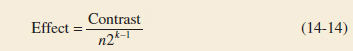
Contrasts are used in calculating both the effect estimates and the sums of squares for A, B, and the AB interaction. For any 2k design with n replicates, the effect estimates are computed from
Relationship Between a Contrast and an Effect
![]() TABLE • 14-12 Signs for Effects in the 22 Design
TABLE • 14-12 Signs for Effects in the 22 Design
and the sum of squares for any effect is
Sum of Squares for an Effect
![]()
One degree of freedom is associated with each effect (two levels minus one) so that the mean squared error of each effect equals the sum of squares. The analysis of variance is completed by computing the total sum of squares SST (with 4n − 1 degrees of freedom) as usual, and obtaining the error sum of squares SSE (with 4(n − 1) degrees of freedom) by subtraction.
Example 14-3 Epitaxial Process An article in the AT&T Technical Journal (March/April 1986, Vol. 65, pp. 39–50) describes the application of two-level factorial designs to integrated circuit manufacturing. A basic processing step in this industry is to grow an epitaxial layer on polished silicon wafers. The wafers are mounted on a susceptor and positioned inside a bell jar. Chemical vapors are introduced through nozzles near the top of the jar. The susceptor is rotated, and heat is applied. These conditions are maintained until the epitaxial layer is thick enough.
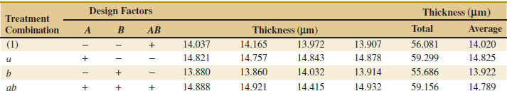
Refer to Table 14-13 for the results of a 22 factorial design with n = 4 replicates using the factors A = deposition time and B = arsenic flow rate. The two levels of deposition time are − = short and + = long, and the two levels of arsenic flow rate are − = 55% and + = 59%. The response variable is epitaxial layer thickness (μm). We may find the estimates of the effects using Equations 14-11, 14-12, and 14-13 as follows:
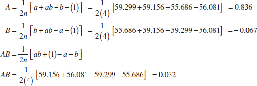
The numerical estimates of the effects indicate that the effect of deposition time is large and has a positive direction (increasing deposition time increases thickness), because changing deposition time from low to high changes the mean epitaxial layer thickness by 0.836 μm. The effects of arsenic flow rate (B) and the AB interaction appear small.
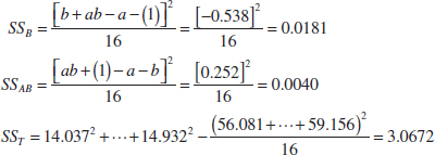
The importance of these effects may be confirmed with the analysis of variance. The sums of squares for A, B, and AB are computed as follows:
![]()
![]() TABLE • 14-13 The 22 Design for the Epitaxial Process Experiment
TABLE • 14-13 The 22 Design for the Epitaxial Process Experiment
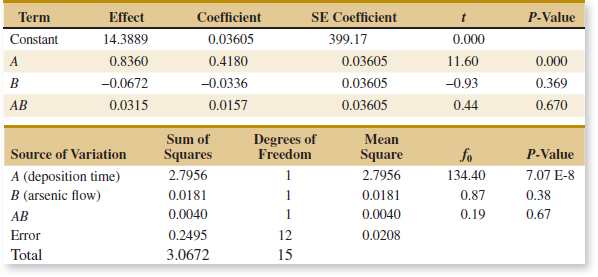
Practical Interpretation: The analysis of variance is summarized in the bottom half of Table 14-14 and confirms our conclusions obtained by examining the magnitude and direction of the effects. Deposition time is the only factor that significantly affects epitaxial layer thickness, and from the direction of the effect estimates, we know that longer deposition times lead to thicker epitaxial layers.
Models and Residual Analysis
It is easy to obtain a model for the response and residuals from a 2k design by fitting a regression model to the data. For the epitaxial process experiment, the regression model is
![]()
because the only active variable is deposition time, which is represented by a coded variable x1. The low and high levels of deposition time are assigned values x1 = −1 and x1 = +1, respectively. The least squares fitted model is
![]()
where the intercept ![]() 0 is the grand average of all 16 observations (
0 is the grand average of all 16 observations (![]() ) and the slope
) and the slope ![]() 1 is one-half the effect estimate for deposition time. The regression coefficient is one-half the effect estimate because regression coefficients measure the effect of a unit change in x1 on the mean of Y, and the effect estimate is based on a two-unit change from −1 to +1.
1 is one-half the effect estimate for deposition time. The regression coefficient is one-half the effect estimate because regression coefficients measure the effect of a unit change in x1 on the mean of Y, and the effect estimate is based on a two-unit change from −1 to +1.
A coefficient relates a factor to the response and, similar to regression analysis, interest centers on whether or not a coefficient estimate is significantly different from zero. Each effect estimate in Equations 14-11 through 14-13 is the difference between two averages (that we denote in general as ![]() + −
+ − ![]() −). In a 2k experiment with n replicates, half the observations appear in each average so that there are n2k−1 observations in each. The associated coefficient estimate, say
−). In a 2k experiment with n replicates, half the observations appear in each average so that there are n2k−1 observations in each. The associated coefficient estimate, say ![]() , equals half the associated effect estimate so that
, equals half the associated effect estimate so that
![]() TABLE • 14-14 Analysis for the Epitaxial Process Experiment
TABLE • 14-14 Analysis for the Epitaxial Process Experiment
![]()
The standard error of ![]() equals half the standard error of the effect, and an effect is simply the difference between two averages. Therefore,
equals half the standard error of the effect, and an effect is simply the difference between two averages. Therefore,
Standard Error of a Coefficient
![]()
where ![]() is estimated from the square root of mean square error. A t-test for a coefficient can also be used to test the significance of an effect. The t-statistic to test H0: β = 0 in a 2k experiment is
is estimated from the square root of mean square error. A t-test for a coefficient can also be used to test the significance of an effect. The t-statistic to test H0: β = 0 in a 2k experiment is
t-statistic for a Coefficient
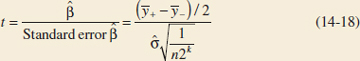
with degrees of freedom equal to those associated with mean square error. This statistic is similar to a two-sample t-test, but σ is estimated from root mean square error. The estimate ![]() accounts for the multiple treatments in an experiment and generally differs from the estimate used in a two-sample t-test.
accounts for the multiple treatments in an experiment and generally differs from the estimate used in a two-sample t-test.
For example, for the epitaxial process experiment in Example 14-3, the effect of A is 0.836. Therefore, the coefficient for A is 0.836/2 = 0.418. Furthermore, ![]() 2 = 0.0208 from the mean squared error in the ANOVA table. Therefore, the standard error of a coefficient is
2 = 0.0208 from the mean squared error in the ANOVA table. Therefore, the standard error of a coefficient is ![]() = 0.03605, and the t-statistic for factor A is 0.418/0.03605 = 11.60. The upper half of Table 14-14 shows the results for the other coefficients. Notice that the P-values obtained from the t-tests equal those in the ANOVA table (aside from rounding). The analysis of a 0k design through coefficient estimates and t-tests is similar to the approach used in regression analysis. Consequently, it might be easier to interpret results from this perspective. Computer software often generates output in this format.
= 0.03605, and the t-statistic for factor A is 0.418/0.03605 = 11.60. The upper half of Table 14-14 shows the results for the other coefficients. Notice that the P-values obtained from the t-tests equal those in the ANOVA table (aside from rounding). The analysis of a 0k design through coefficient estimates and t-tests is similar to the approach used in regression analysis. Consequently, it might be easier to interpret results from this perspective. Computer software often generates output in this format.
Some algebra can be used to show that for a 2k experiment, the square of the t-statistic for the coefficient test equals the F-statistic used for the effect test in the analysis of variance. In Table 14-14, the square of the t-statistic for factor A is 11.5962 = 134.47, and this equals the F-statistic for factor A in the ANOVA. Also, the square of a t random variable with d degrees of freedom is an F random variable with 1 numerator and d denominator degrees of freedom. Thus, the test that compares the absolute value of the t-statistic to the t distribution is equivalent to the F-test, and either method may be used to test an effect.
The least squares fitted model can also be used to obtain the predicted values at the four points that form the corners of the square in the design. For example, consider the point with low deposition time (x1 = −1) and low arsenic flow rate. The predicted value is
![]()
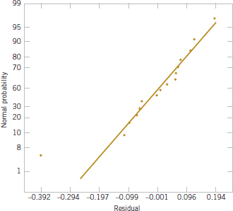
FIGURE 14-16 Normal probability plot of residuals for the epitaxial process experiment.
and the residuals for the four runs at that design point are
The remaining predicted values and residuals at the other three design points are calculated in a similar manner.
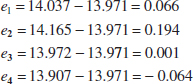
A normal probability plot of these residuals is shown in Fig. 14-16. This plot indicates that one residual e15 = −0.392 is an outlier. Examining the four runs with high deposition time and high arsenic flow rate reveals that observation y15 = 14.415 is considerably smaller than the other three observations at that treatment combination. This adds some additional evidence to the tentative conclusion that observation 15 is an outlier. Another possibility is that some process variables affect the variability in epitaxial layer thickness. If we could discover which variables produce this effect, we could perhaps adjust these variables to levels that would minimize the variability in epitaxial layer thickness. This could have important implications in subsequent manufacturing stages. Figures 14-17 and 14-18 are plots of residuals versus deposition time and arsenic flow rate, respectively. Except for the unusually large residual associated with y15, there is no strong evidence that either deposition time or arsenic flow rate influences the variability in epitaxial layer thickness.
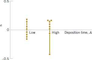
FIGURE 14-17 Plot of residuals versus deposition time.
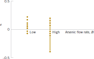
FIGURE 14-18 Plot of residuals versus arsenic flow rate.
Figure 14-19 shows the standard deviation of epitaxial layer thickness at all four runs in the 22 design. These standard deviations were calculated using the data in Table 14-13. Notice that the standard deviation of the four observations with A and B at the high level is considerably larger than the standard deviations at any of the other three design points. Most of this difference is attributable to the unusually low thickness measurement associated with y15. The standard deviation of the four observations with A and B at the low level is also somewhat larger than the standard deviations at the remaining two runs. This could indicate that other process variables not included in this experiment may affect the variability in epitaxial layer thickness. Another experiment to study this possibility, involving other process variables, could be designed and conducted. (The original paper in the AT&T Technical Journal shows that two additional factors not considered in this example affect process variability.)
14-5.2 2k DESIGN FOR k ≥ 3 FACTORS
The methods presented in the previous section for factorial designs with k = 2 factors each at two levels can be easily extended to more than two factors. For example, consider k = 3 factors, each at two levels. This design is a 23 factorial design, and it has eight runs or treatment combinations. Geometrically, the design is a cube as shown in Fig. 14-20(a) with the eight runs forming the corners of the cube. Figure 14-20(b) lists the eight runs in a table with each row representing one of the runs and the − and + settings indicating the low and high levels for each of the three factors. This table is sometimes called the design matrix. This design allows three main effects (A, B and C) to be estimated along with three two-factor interactions (AB, AC, and BC) and a three-factor interaction (ABC).
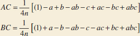
The main effects can easily be estimated. Remember that the lowercase letters (1), a, b, ab, c, ac, bc, and abc represent the total of all n replicates at each of the eight runs in the design. As in Fig. 14-21(a), the main effect of A can be estimated by averaging the four treatment combinations on the right-hand side of the cube where A is at the high level and by subtracting from this quantity the average of the four treatment combinations on the left-hand side of the cube where A is at the low level. This gives
![]()
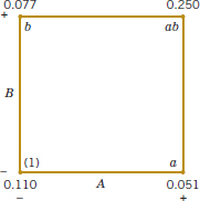
FIGURE 14-19 The standard deviation of epitaxial layer thickness at the four runs in the 22 design.
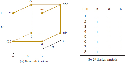
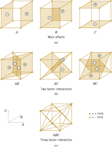
FIGURE 14-21 Geometric presentation of contrasts corresponding to the main effects and interaction in the 23 design. (a) Main effects. (b) Two-factor interactions. (c) Three-factor interaction.
This equation can be rearranged as
Main Effect of Factor A:23 Design
![]()
In a similar manner, the effect of B is the difference in averages between the four treatment combinations in the back face of the cube [Fig. 14-19(a)], and the four in the front. This yields
Main Effect of Factor B:23 Design
![]()
The effect of C is the difference in average response between the four treatment combinations in the top face of the cube in Figure 14-19(a) and the four in the bottom, that is,
Main Effect of Factor C:23 Design
![]()
The two-factor interaction effects may be computed easily. A measure of the AB interaction is the difference between the average A effects at the two levels of B. By convention, one-half of this difference is called the AB interaction. Symbolically,
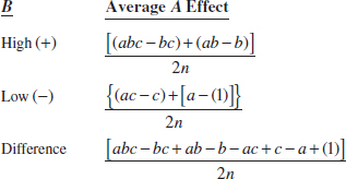
Because the AB interaction is one-half of this difference,
Two-Factor Interaction Effects: 23 Design
![]()
We could write the AB effect as follows:
![]()
In this form, the AB interaction can easily be seen to be the difference in averages between runs on two diagonal planes in the cube in Fig. 14-19(b). Using similar logic and referring to Fig. 14-19(b), we find that the AC and BC interactions are
Two-Factor Interaction Effect: 23 Design
The ABC interaction is defined as the average difference between the AB interaction for the two different levels of C. Thus,
![]()
or
Three-Factor Interaction Effect: 23 Design
![]()
As before, we can think of the ABC interaction as the difference in two averages. If the runs in the two averages are isolated, they define the vertices of the two tetrahedra that comprise the cube in Fig. 14-21(c).
![]() TABLE • 14-15 Algebraic Signs for Calculating Effects in the 23 Design
TABLE • 14-15 Algebraic Signs for Calculating Effects in the 23 Design
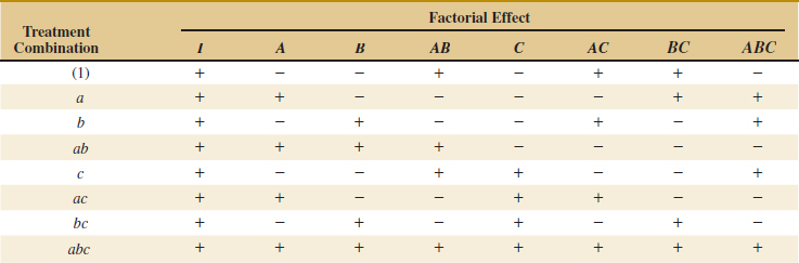
In the equations for the effects, the quantities in brackets are contrasts in the treatment combinations. A table of plus and minus signs can be developed from the contrasts and is shown in Table 14-15. Signs for the main effects are determined directly from the test matrix in Figure 14-20(b). Once the signs for the main effect columns have been established, the signs for the remaining columns can be obtained by multiplying the appropriate main effect row by row. For example, the signs in the AB column are the products of the A and B column signs in each row. The contrast for any effect can easily be obtained from this table.
Table 14-15 has several interesting properties:
- Except for the identity column I, each column has an equal number of plus and minus signs.
- The sum of products of signs in any two columns is zero; that is, the columns in the table are orthogonal.
- Multiplying any column by column I leaves the column unchanged; that is, I is an identity element.
- The product of any two columns yields a column in the table, for example A × B = AB, and AB × ABC = A2B2C = C because any column multiplied by itself is the identity column.
The estimate of any main effect or interaction in a 2k design is determined by multiplying the treatment combinations in the first column of the table by the signs in the corresponding main effect or interaction column, by adding the result to produce a contrast, and then by dividing the contrast by one-half the total number of runs in the experiment.
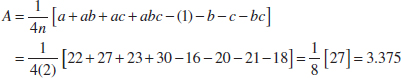
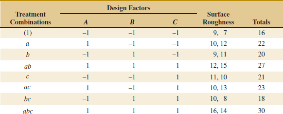
EXAMPLE 14-4 Surface Roughness Consider the surface roughness experiment originally described in Example 14-2. This is a 23 factorial design in the factors feed rate (A), depth of cut (B), and tool angle (C), with n = 2 replicates. Table 14-16 presents the observed surface roughness data.
The effect of A, for example, is
![]() TABLE • 14-16 Surface Roughness Data for Example 14-4
TABLE • 14-16 Surface Roughness Data for Example 14-4
and the sum of squares for A is found using Equation 14-15:
![]()
It is easy to verify that the other effects are
Examining the magnitude of the effects clearly shows that feed rate (factor A) is dominant, followed by depth of cut (B) and the AB interaction, although the interaction effect is relatively small. The analysis, summarized in Table 14-17, confirms our interpretation of the effect estimates.
The output from the computer software for this experiment is shown in Table 14-18. The upper portion of the table displays the effect estimates and regression coefficients for each factorial effect. To illustrate, for the main effect of feed, the computer output reports t = 4.32 (with 8 degrees of freedom), and t2 = (4.32)2 = 18.66, which is approximately equal to the F-ratio for feed reported in Table 14-18 (F = 18.69). This F-ratio has one numerator and 8 denominator degrees of freedom.
The lower panel of the computer output in Table 14-18 is an analysis of variance summary focusing on the types of terms in the model. A regression model approach is used in the presentation. You might find it helpful to review Section 12-2.2, particularly the material on the partial F-test. The row entitled “main effects” under source refers to the three main effects feed, depth, and angle, each having a single degree of freedom, giving the total 3 in the column headed “DF.” The column headed “Seq SS” (an abbreviation for sequential sum of squares) reports how much the model sum of squares increases when each group of terms is added to a model that contains the terms listed above the groups. The first number in the “Seq SS” column presents the model sum of squares for fitting a model having only the three main effects. The row labeled “2-Way Interactions” refers to AB, AC, and BC, and the sequential sum of squares reported here is the increase in the model sum of squares if the interaction terms are added to a model containing only the main effects. Similarly, the sequential sum of squares for the three-way interaction is the increase in the model sum of squares that results from adding the term ABC to a model containing all other effects.
The column headed “Adj SS” (an abbreviation for adjusted sum of squares) reports how much the model sum of squares increases when each group of terms is added to a model that contains all the other terms. Now because any 2k design with an equal number of replicates in each cell is an orthogonal design, the adjusted sum of squares equals the sequential sum of squares. Therefore, the F-tests for each row in the computer analysis of variance in Table 14-18 are testing the significance of each group of terms (main effects, two-factor interactions, and three-factor interactions) as if they were the last terms to be included in the model. Clearly, only the main effect terms are significant. The t-tests on the individual factor effects indicate that feed rate and depth of cut have large main effects, and there may be some mild interaction between these two factors. Therefore, the computer output agrees with the results given previously.
![]() TABLE • 14-17 Analysis for the Surface Roughness Experiment
TABLE • 14-17 Analysis for the Surface Roughness Experiment
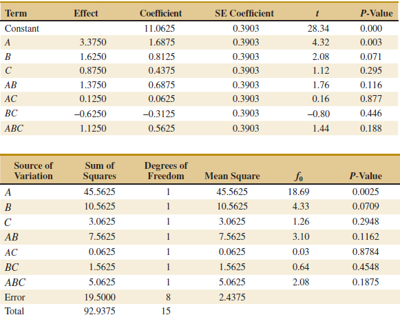
![]() TABLE • 14-18 Computer Analysis for the Surface Roughness Experiment in Example 14-4
TABLE • 14-18 Computer Analysis for the Surface Roughness Experiment in Example 14-4
Models and Residual Analysis
We may obtain the residuals from a 2k design by using the method demonstrated earlier for the 22 design. As an example, consider the surface roughness experiment. The three largest effects are A, B, and the AB interaction. The regression model used to obtain the predicted values is
![]()
where x1 represents factor A, x2 represents factor B, and x1x2 represents the AB interaction. The regression coefficients β1, β2, and β12 are estimated by one-half the corresponding effect estimates, and β0 is the grand average. Thus,
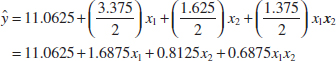
Note that the regression coefficients are presented in the upper panel of Table 14-18. The predicted values would be obtained by substituting the low and high levels of A and B into this equation. To illustrate this, at the treatment combination where A, B, and C are all at the low level, the predicted value is
![]()
Because the observed values at this run are 9 and 7, the residuals are 9 − 9.25 = −0.25 and 7 − 9.25 = −2.25. Residuals for the other 14 runs are obtained similarly.
See a normal probability plot of the residuals in Fig. 14-22. Because the residuals lie approximately along a straight line, we do not suspect any problem with normality in the data. There are no indications of severe outliers. It would also be helpful to plot the residuals versus the predicted values and against each of the factors A, B, and C.
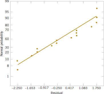
FIGURE 14-22 Normal probability plot of residuals from the surface roughness experiment.
Projection of 2k Designs
Any 2k design collapses or projects into another 2k design in fewer variables if one or more of the original factors are dropped. Sometimes this can provide additional insight into the remaining factors. For example, consider the surface roughness experiment. Because factor C and all its interactions are negligible, we could eliminate factor C from the design. The result is to collapse the cube in Fig. 14-20 into a square in the A − B plane; therefore, each of the four runs in the new design has four replicates. In general, if we delete h factors so that r = k − h factors remain, the original 2k design with n replicates projects into a 2r design with n2h replicates.
14-5.3 SINGLE REPLICATE OF THE 2k DESIGN
As the number of factors in a factorial experiment increases, the number of effects that can be estimated also increases. For example, a 24 experiment has 4 main effects, 6 two-factor interactions, 4 three-factor interactions, and 1 four-factor interaction, and a 26 experiment has 6 main effects, 15 two-factor interactions, 20 three-factor interactions, 15 four-factor interactions, 6 five-factor interactions, and 1 six-factor interaction. In most situations, the sparsity of effects principle applies; that is, the system is usually dominated by the main effects and low-order interactions. The three-factor and higher order interactions are usually negligible. Therefore, when the number of factors is moderately large, say, k ≥ 4 or 5, a common practice is to run only a single replicate of the 2k design and then pool or combine the higher order interactions as an estimate of error. Sometimes a single replicate of a 2k design is called an unreplicated 2k factorial design.
When analyzing data from unreplicated factorial designs, occasionally real high-order interactions occur. The use of an error mean square obtained by pooling high-order interactions is inappropriate in these cases. A simple method of analysis can be used to overcome this problem. Construct a plot of the estimates of the effects on a normal probability scale. The effects that are negligible are normally distributed with mean zero and variance σ2 and tend to fall along a straight line on this plot, whereas significant effects has nonzero means and will not lie along the straight line. We illustrate this method in Example 14-5.
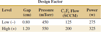
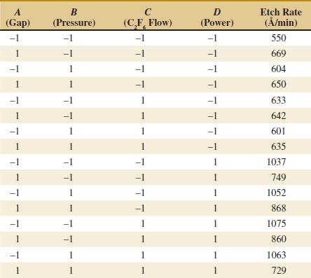
Example 14-5 Plasma Etch An article in Solid State Technology [“Orthogonal Design for Process Optimization and Its Application in Plasma Etching” (May 1987, pp. 127–132)] describes the application of factorial designs in developing a nitride etch process on a single-wafer plasma etcher. The process uses C2F6 as the reactant gas. It is possible to vary the gas flow, the power applied to the cathode, the pressure in the reactor chamber, and the spacing between the anode and the cathode (gap). Several response variables would usually be of interest in this process, but in this example, we concentrate on etch rate for silicon nitride.
We use a single replicate of a 24 design to investigate this process. Because it is unlikely that the three- and four-factor interactions are significant, we tentatively plan to combine them as an estimate of error. The factor levels used in the design follow:
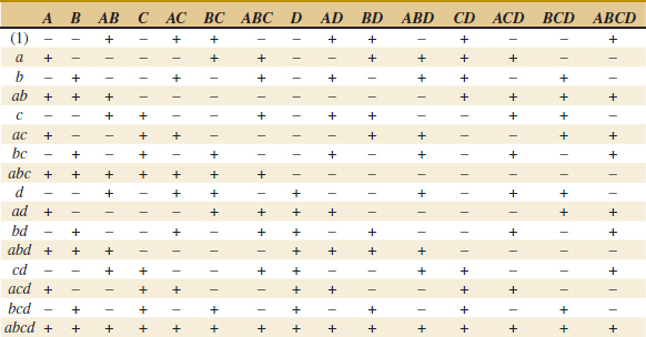
Refer to Table 14-19 for the data from the 16 runs of the 24 design. Table 14-20 is the table of plus and minus signs for the 24 design. The signs in the columns of this table can be used to estimate the factor effects. For example, the estimate of factor A is
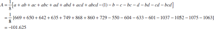
Thus, the effect of increasing the gap between the anode and the cathode from 0.80 to 1.20 centimeters is to decrease the etch rate by 101.625 angstroms per minute.
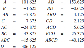
It is easy to verify (using computer software, for example) that the complete set of effect estimates is
The normal probability plot of these effects from the plasma etch experiment is shown in Fig. 14-23. Clearly, the main effects of A and D and the AD interaction are significant because they fall far from the line passing through the other points. The analysis, summarized in Table 14-21, confirms these findings. Notice that in the analysis of variance we have pooled the three- and four-factor interactions to form the error mean square. If the normal probability plot had indicated that any of these interactions were important, they would not have been included in the error term.
![]() TABLE • 14-19 The 24 Design for the Plasma Etch Experiment
TABLE • 14-19 The 24 Design for the Plasma Etch Experiment
![]() TABLE • 14-20 Contrast Constants for the 24 Design
TABLE • 14-20 Contrast Constants for the 24 Design
![]() TABLE • 14-21 Analysis for the Plasma Etch Experiment
TABLE • 14-21 Analysis for the Plasma Etch Experiment
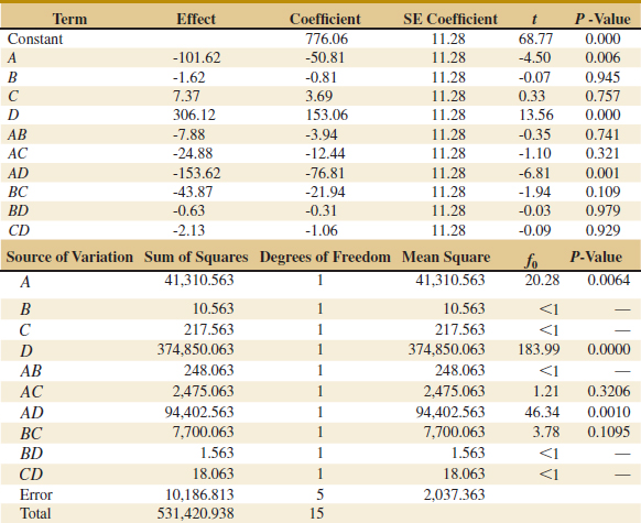
Practical Interpretation: Because A = −101.625, the effect of increasing the gap between the cathode and anode is to decrease the etch rate. However, D = 306.125; thus, applying higher power levels increase the etch rate. Figure 14-24 is a plot of the AD interaction. This plot indicates that the effect of changing the gap width at low power settings is small but that increasing the gap at high power settings dramatically reduces the etch rate. High etch rates are obtained at high power settings and narrow gap widths.
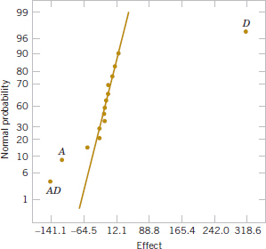
FIGURE 14-23 Normal probability plot of effects from the plasma etch experiment.
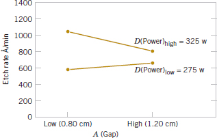
FIGURE 14-24 AD (gap-power) interaction from the plasma etch experiment.
The residuals from the experiment in Example 14-5 can be obtained from the regression model
![]()
For example, when both A and D are at the low level, the predicted value is
![]()
and the four residuals at this treatment combination are
![]()
The residuals at the other three treatment combinations (A high, D low), (A low, D high), and (A high, D high) are obtained similarly. A normal probability plot of the residuals is shown in Fig. 14-25. The plot is satisfactory.
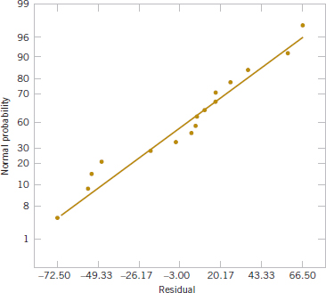
FIGURE 14-25 Normal probability plot of residuals from the plasma etch experiment.
14-5.4 ADDITION OF CENTER POINTS TO A 2k DESIGN
A potential concern in the use of two-level factorial designs is the assumption of linearity in the factor effects. Of course, perfect linearity is unnecessary, and the 2k system works quite well even when the linearity assumption holds only approximately. However, a method of replicating certain points in the 2k factorial provides protection against curvature and allows an independent estimate of error to be obtained. The method consists of adding center points to the 2k design. These consist of nC replicates run at the point xi = 0 (i = 1, 2,..., k). One important reason for adding the replicate runs at the design center is that center points do not affect the usual effects estimates in a 2k design. We assume that the k factors are quantitative.
To illustrate the approach, consider a 22 design with one observation at each of the factorial points (−, −),(+, −),(−, +), and (+, +) and nC observations at the center points (0, 0). Figure 14-26 illustrates the situation. Let ![]() F be the average of the four runs at the four factorial points, and let
F be the average of the four runs at the four factorial points, and let ![]() C be the average of the nC run at the center point. If the difference
C be the average of the nC run at the center point. If the difference ![]() F −
F − ![]() C is small, the center points lie on or near the plane passing through the factorial points, and there is no curvature. On the other hand, if
C is small, the center points lie on or near the plane passing through the factorial points, and there is no curvature. On the other hand, if ![]() F −
F − ![]() C is large, curvature is present.
C is large, curvature is present.
Similar to factorial effects, a test for curvature can be based on a F-statistic or an equivalent t-statistic. A single degree-of-freedom sum of squares for curvature is compared to MSE to produce the F-statistic. Alternatively, a t-statistic similar to the one used to compare two means can be computed. A coefficient for curvature is defined to be ![]() F −
F − ![]() C, and σ is estimated by the square root of MSE. This leads to the following formulas:
C, and σ is estimated by the square root of MSE. This leads to the following formulas:
Curvature Sum of Squares and t-Statistic
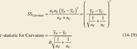
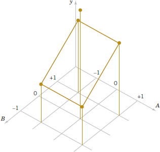
FIGURE 14-26 A 22 design with center points.
where, in general, nF is the number of factorial design points. The SSCurvature may be compared to the error mean square to produce the F-test for curvature. Notice that, similar to the test for other effects, the square of the t-statistic equals the F-statistic.
When points are added to the center of the 2k design, the model we may entertain is
![]()
where the βjj are pure quadratic effects. The test for curvature actually tests the hypotheses
![]()
Furthermore, if the factorial points in the design are unreplicated, we may use the nC center points to construct an estimate of error with nC − 1 degrees of freedom.
Example 14-6 Process Yield A chemical engineer is studying the percentage of conversion or yield of a process. There are two variables of interest, reaction time and reaction temperature. Because she is uncertain about the assumption of linearity over the region of exploration, the engineer decides to conduct a 22 design (with a single replicate of each factorial run) augmented with five center points. The design and the yield data are shown in Fig. 14-27.
Table 14-22 summarizes the analysis for this experiment. The mean square error is calculated from the center points as follows:
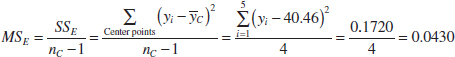
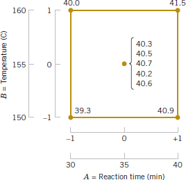
FIGURE 14-27 The 22 design with five center points for the process yield experiment in Example 14-6.
![]() TABLE • 14-22 Analysis for the Process Yield Experiment with Center Points
TABLE • 14-22 Analysis for the Process Yield Experiment with Center Points
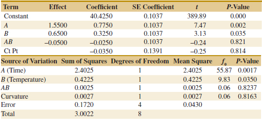
The average of the points in the factorial portion of the design is ![]() F = 40.425, and the average of the points at the center is
F = 40.425, and the average of the points at the center is ![]() C = 40.46. The difference
C = 40.46. The difference ![]() F −
F − ![]() C = 40.425 − 40.46 = −0.035 appears to be small. The curvature sum of squares in the analysis of variance table is computed from Equation 14-19 as follows:
C = 40.425 − 40.46 = −0.035 appears to be small. The curvature sum of squares in the analysis of variance table is computed from Equation 14-19 as follows:
![]()
The coefficient for curvature is ![]() F −
F − ![]() C = −0.035, and the t-statistic to test for curvature is
C = −0.035, and the t-statistic to test for curvature is

Practical Interpretation: The analysis of variance indicates that both factors exhibit significant main effects, that there is no interaction, and that there is no evidence of curvature in the response over the region of exploration. That is, the null hypothesis H0: ![]() = 0 cannot be rejected.
= 0 cannot be rejected.
Exercises FOR SECTION 14-5
![]() Problem available in WileyPLUS at instructor's discretion.
Problem available in WileyPLUS at instructor's discretion.
![]() Go Tutorial Tutoring problem available in WileyPLUS at instructor's discretion.
Go Tutorial Tutoring problem available in WileyPLUS at instructor's discretion.
![]() 14-14.
14-14. ![]() An engineer is interested in the effect of cutting speed (A), metal hardness (B), and cutting angle (C) on the life of a cutting tool. Two levels of each factor are chosen, and two replicates of a 23 factorial design are run. The tool life data (in hours) are shown in the following table.
An engineer is interested in the effect of cutting speed (A), metal hardness (B), and cutting angle (C) on the life of a cutting tool. Two levels of each factor are chosen, and two replicates of a 23 factorial design are run. The tool life data (in hours) are shown in the following table.
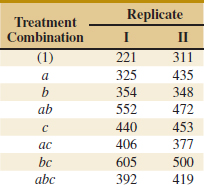
(a) Analyze the data from this experiment.
(b) Find an appropriate regression model that explains tool life in terms of the variables used in the experiment.
(c) Analyze the residuals from this experiment.
![]() 14-15. Four factors are thought to influence the taste of a soft-drink beverage: type of sweetener (A), ratio of syrup to water (B), carbonation level (C), and temperature (D). Each factor can be run at two levels, producing a 24 design. At each run in the design, samples of the beverage are given to a test panel consisting of 20 people. Each tester assigns the beverage a point score from 1 to 10. Total score is the response variable, and the objective is to find a formulation that maximizes total score. Two replicates of this design are run, and the results are shown in the table. Analyze the data and draw conclusions. Use a = 0.05 in the statistical tests.
14-15. Four factors are thought to influence the taste of a soft-drink beverage: type of sweetener (A), ratio of syrup to water (B), carbonation level (C), and temperature (D). Each factor can be run at two levels, producing a 24 design. At each run in the design, samples of the beverage are given to a test panel consisting of 20 people. Each tester assigns the beverage a point score from 1 to 10. Total score is the response variable, and the objective is to find a formulation that maximizes total score. Two replicates of this design are run, and the results are shown in the table. Analyze the data and draw conclusions. Use a = 0.05 in the statistical tests.
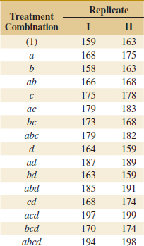
![]()
14-16. The following data represent a single replicate of a 25 design that is used in an experiment to study the compressive strength of concrete. The factors are mix (A), time (B), laboratory (C), temperature (D), and drying time (E).
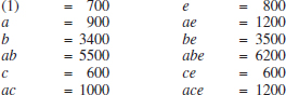
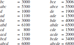
(a) Estimate the factor effects.
(b) Which effects appear important? Use a normal probability plot.
(c) If it is desirable to maximize the strength, in which direction would you adjust the process variables?
(d) Analyze the residuals from this experiment.
![]() 14-17.
14-17. ![]() An article in IEEE Transactions on Semiconductor Manufacturing (1992, Vol. 5, pp. 214–222) described an experiment to investigate the surface charge on a silicon wafer. The factors thought to influence induced surface charge are cleaning method (spin rinse dry or SRD and spin dry or SD) and the position on the wafer where the charge was measured. The surface charge (× 1011 q/cm3) response data follow:
An article in IEEE Transactions on Semiconductor Manufacturing (1992, Vol. 5, pp. 214–222) described an experiment to investigate the surface charge on a silicon wafer. The factors thought to influence induced surface charge are cleaning method (spin rinse dry or SRD and spin dry or SD) and the position on the wafer where the charge was measured. The surface charge (× 1011 q/cm3) response data follow:
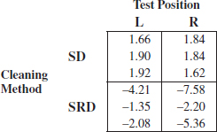
(a) Estimate the factor effects.
(b) Which factors appear important? Use α = 0.05.
(c) Analyze the residuals from this experiment.
![]() 14-18.
14-18. ![]() An article in Oikos: A Journal of Ecology [“Regulation of Root Vole Population Dynamics by Food Supply and Predation: A Two-Factor Experiment” (2005, Vol. 109, pp. 387–395)] investigated how food supply interacts with predation in the regulation of root vole (Microtus oeconomus Pallas) population dynamics. A replicated two-factor field experiment manipulating both food supply and predation condition for root voles was conducted. Four treatments were applied: −P, +F (no-predator, food-supplemented); +P, +F (predator-access, food-supplemented); −P, −F (no-predator, nonsupplemented); +P, −F (predator-access, food-supplemented). The population density of root voles (voles ha−1) for each treatment combination follows.
An article in Oikos: A Journal of Ecology [“Regulation of Root Vole Population Dynamics by Food Supply and Predation: A Two-Factor Experiment” (2005, Vol. 109, pp. 387–395)] investigated how food supply interacts with predation in the regulation of root vole (Microtus oeconomus Pallas) population dynamics. A replicated two-factor field experiment manipulating both food supply and predation condition for root voles was conducted. Four treatments were applied: −P, +F (no-predator, food-supplemented); +P, +F (predator-access, food-supplemented); −P, −F (no-predator, nonsupplemented); +P, −F (predator-access, food-supplemented). The population density of root voles (voles ha−1) for each treatment combination follows.
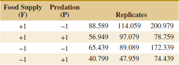
(a) What is an appropriate statistical model for this experiment?
(b) Analyze the data and draw conclusions.
(c) Analyze the residuals from this experiment. Are there any problems with model adequacy?
![]()
14-19. ![]() An experiment was run in a semiconductor fabrication plant in an effort to increase yield. Five factors, each at two levels, were studied. The factors (and levels) were A = aperture setting (small, large), B = exposure time (20% below nominal, 20% above nominal), C = development time (30 and 45 seconds), D = mask dimension (small, large), and E = etch time (14.5 and 15.5 minutes). The following unreplicated 25 design was run:
An experiment was run in a semiconductor fabrication plant in an effort to increase yield. Five factors, each at two levels, were studied. The factors (and levels) were A = aperture setting (small, large), B = exposure time (20% below nominal, 20% above nominal), C = development time (30 and 45 seconds), D = mask dimension (small, large), and E = etch time (14.5 and 15.5 minutes). The following unreplicated 25 design was run:
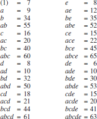
(a) Construct a normal probability plot of the effect estimates. Which effects appear to be large?
(b) Conduct an analysis of variance to confirm your findings for part (a).
(c) Construct a normal probability plot of the residuals. Is the plot satisfactory?
(d) Plot the residuals versus the predicted yields and versus each of the five factors. Comment on the plots.
(e) Interpret any significant interactions.
(f) What are your recommendations regarding process operating conditions?
(g) Project the 25 design in this problem into a 2r for r < 5 design in the important factors. Sketch the design and show the average and range of yields at each run. Does this sketch aid in data interpretation?
![]()
14-20. An experiment described by M. G. Natrella in the National Bureau of Standards' Handbook of Experimental Statistics (1963, No. 91) involves flame-testing fabrics after applying fire-retardant treatments. The four factors considered are type of fabric (A), type of fire-retardant treatment (B), laundering condition (C—the low level is no laundering, the high level is after one laundering), and method of conducting the flame test (D). All factors are run at two levels, and the response variable is the inches of fabric burned on a standard size test sample. The data are:
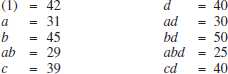
(a) Estimate the effects and prepare a normal plot of the effects.
(b) Construct an analysis of variance table based on the model tentatively identified in part (a).
(c) Construct a normal probability plot of the residuals and comment on the results.
![]() 14-21.
14-21. ![]() Consider the data from Exercise 14-14. Suppose that the data from the second replicate were not available. Analyze the data from replicate I only and comment on your findings.
Consider the data from Exercise 14-14. Suppose that the data from the second replicate were not available. Analyze the data from replicate I only and comment on your findings.
![]() 14-22. A 24 factorial design was run in a chemical process. The design factors are A = time, B = concentration, C = pressure, and D = temperature. The response variable is yield. The data follow:
14-22. A 24 factorial design was run in a chemical process. The design factors are A = time, B = concentration, C = pressure, and D = temperature. The response variable is yield. The data follow:

(a) Estimate the factor effects. Based on a normal probability plot of the effect estimates, identify a model for the data from this experiment.
(b) Conduct an ANOVA based on the model identified in part (a). What are your conclusions?
(c) Analyze the residuals and comment on model adequacy.
(d) Find a regression model to predict yield in terms of the actual factor levels.
(e) Can this design be projected into a 23 design with two replicates? If so, sketch the design and show the average and range of the two yield values at each cube corner. Discuss the practical value of this plot.
![]() 14-23.
14-23. ![]() An experiment has run a single replicate of a 24 design and calculated the following factor effects:
An experiment has run a single replicate of a 24 design and calculated the following factor effects:
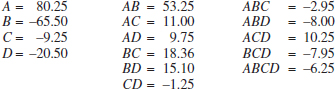
(a) Construct a normal probability plot of the effects.
(b) Identify a tentative model, based on the plot of effects in part (a).
(c) Estimate the regression coefficients in this model, assuming that ![]() = 400.
= 400.
![]()
14-24. A two-level factorial experiment in four factors was conducted by Chrysler and described in the article “Sheet Molded Compound Process Improvement” by P. I. Hsieh and D. E. Goodwin (Fourth Symposium on Taguchi Methods, American Supplier Institute, Dearborn, MI, 1986, pp. 13–21). The purpose was to reduce the number of defects in the finish of sheet-molded grill opening panels. A portion of the experimental design, and the resulting number of defects, yi observed on each run is shown in the following table. This is a single replicate of the 24 design.
(a) Estimate the factor effects and use a normal probability plot to tentatively identify the important factors.
(b) Fit an appropriate model using the factors identified in part (a).
(c) Plot the residuals from this model versus the predicted number of defects. Also prepare a normal probability plot of the residuals. Comment on the adequacy of these plots.
(d) The following table also shows the square root of the number of defects. Repeat parts (a) and (c) of the analysis using the square root of the number of defects as the response. Does this change the conclusions?
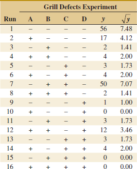
14-25. ![]() Consider a 22 factorial experiment with four center points. The data are (1) = 21, a = 125, b = 154, ab = 352, and the responses at the center point are 92, 130, 98, 152. Compute an ANOVA with the sum of squares for curvature and conduct an F-test for curvature. Use α = 0.05.
Consider a 22 factorial experiment with four center points. The data are (1) = 21, a = 125, b = 154, ab = 352, and the responses at the center point are 92, 130, 98, 152. Compute an ANOVA with the sum of squares for curvature and conduct an F-test for curvature. Use α = 0.05.
![]()
14-26. ![]() Consider the experiment in Exercise 14-16. Suppose that a center point with five replicates is added to the factorial runs and the responses are 2800, 5600, 4500, 5400, 3600. Compute an ANOVA with the sum of squares for curvature and conduct an F-test for curvature. Use α = 0.05.
Consider the experiment in Exercise 14-16. Suppose that a center point with five replicates is added to the factorial runs and the responses are 2800, 5600, 4500, 5400, 3600. Compute an ANOVA with the sum of squares for curvature and conduct an F-test for curvature. Use α = 0.05.
![]() 14-27. Consider the experiment in Exercise 14-19. Suppose that a center point with five replicates is added to the factorial runs and the responses are 45, 40, 41, 47, and 43.
14-27. Consider the experiment in Exercise 14-19. Suppose that a center point with five replicates is added to the factorial runs and the responses are 45, 40, 41, 47, and 43.
(a) Estimate the experimental error using the center points. Compare this to the estimate obtained originally in Exercise 14-19 by pooling apparently nonsignificant effects.
(b) Test for curvature with α = 0.05.
![]() 14-28. An article in Talanta (2005, Vol. 65, pp. 895–899) presented a 23 factorial design to find lead level by using flame atomic absorption spectrometry (FAAS). The data are in the following table.
14-28. An article in Talanta (2005, Vol. 65, pp. 895–899) presented a 23 factorial design to find lead level by using flame atomic absorption spectrometry (FAAS). The data are in the following table.
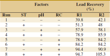
The factors and levels are in the following table.

(a) Construct a normal probability plot of the effect estimates. Which effects appear to be large?
(b) Conduct an analysis of variance to confirm your findings for part (a).
(c) Analyze the residuals from this experiment. Are there any problems with model adequacy?
![]() 14-29. An experiment to study the effect of machining factors on ceramic strength was described at www.itl.nist.gov/div898/handbook/. Five factors were considered at two levels each: A = Table Speed, B = Down Feed Rate, C = Wheel Grit, D = Direction, E = Batch. The response is the average of the ceramic strength over 15 repetitions. The following data are from a single replicate of a 25 factorial design.
14-29. An experiment to study the effect of machining factors on ceramic strength was described at www.itl.nist.gov/div898/handbook/. Five factors were considered at two levels each: A = Table Speed, B = Down Feed Rate, C = Wheel Grit, D = Direction, E = Batch. The response is the average of the ceramic strength over 15 repetitions. The following data are from a single replicate of a 25 factorial design.
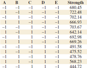
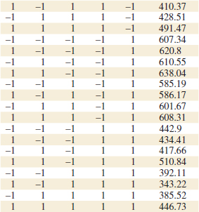
(a) Estimate the factor effects and use a normal probability plot of the effects. Identify which effects appear to be large.
(b) Fit an appropriate model using the factors identified in part (a).
(c) Prepare a normal probability plot of the residuals. Also, plot the residuals versus the predicted ceramic strength. Comment on the adequacy of these plots.
(d) Identify and interpret any significant interactions.
(e) What are your recommendations regarding process operating conditions?
14-30. Consider the following computer output for a 23 factorial experiment.
(a) How many replicates were used in the experiment?
(b) Use the appropriate equation to calculate the standard error of a coefficient.
(c) Calculate the entries marked with “?” in the output.
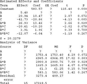
14-31. Consider the following computer output for one replicate of a 24 factorial experiment.
(a) What effects are used to estimate error?
(b) Calculate the entries marked with “?” in the output.
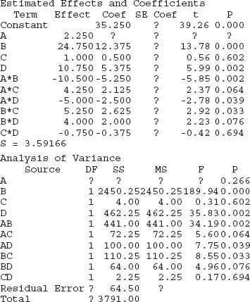
![]() 14-32. An article in Bioresource Technology (“Influence of Vegetable Oils Fatty-Acid Composition on Biodiesel Optimization,” (2011, Vol. 102(2), pp. 1059–1065)] described an experiment to analyze the influence of the fatty-acid composition on biodiesel. Factors were the concentration of catalyst, amount of methanol, reaction temperature and time, and the design included three center points. Maize oil methyl ester (MME) was recorded as the response. Data follow.
14-32. An article in Bioresource Technology (“Influence of Vegetable Oils Fatty-Acid Composition on Biodiesel Optimization,” (2011, Vol. 102(2), pp. 1059–1065)] described an experiment to analyze the influence of the fatty-acid composition on biodiesel. Factors were the concentration of catalyst, amount of methanol, reaction temperature and time, and the design included three center points. Maize oil methyl ester (MME) was recorded as the response. Data follow.
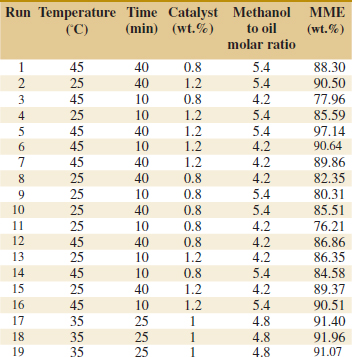
(a) Identify the important effects from a normal probability plot.
(b) Compare the results in the previous part with results that use an error term based on the center points.
(c) Test for curvature.
(d) Analyze the residuals from the model.
![]()
14-33. An article in Analytica Chimica Acta [“Design-of-Experiment Optimization of Exhaled Breath Condensate Analysis Using a Miniature Differential Mobility Spectrometer (DMS)” (2008, Vol. 628(2), pp. 155–161)] examined four parameters that affect the sensitivity and detection of the analytical instruments used to measure clinical samples. They optimized the sensor function using exhaled breath condensate (EBC) samples spiked with acetone, a known clinical biomarker in breath. The following table shows the results for a single replicate of a 24 factorial experiment for one of the outputs, the average amplitude of acetone peak over three repetitions.
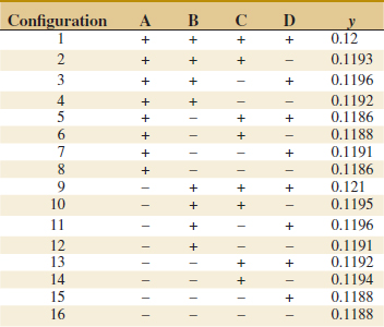
The factors and levels are shown in the following table.
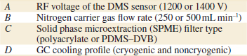
(a) Estimate the factor effects and use a normal probability plot of the effects. Identify which effects appear to be large, and identify a model for the data from this experiment.
(b) Conduct an ANOVA based on the model identified in part (a). What are your conclusions?
(c) Analyze the residuals from this experiment. Are there any problems with model adequacy?
(d) Project the design in this problem into a 2r design for r < 4 in the important factors. Sketch the design and show the average and range of yields at each run. Does this sketch aid in data representation?
![]()
14-34. An article in Journal of Construction Engineering and Management (“Analysis of Earth-Moving Systems Using Discrete—Event Simulation,” 1995, Vol. 121(4), pp. 388–396) considered a replicated two-level factorial experiment to study the factors most important to output in an earth-moving system. Handle the experiment as four replicates of a 24 factorial design with response equal to production rate (m3 / h). The data are shown in the following table.
(a) Estimate the factor effects. Based on a normal probability plot of the effect estimates, identify a model for the data from this experiment.
(b) Conduct an ANOVA based on the model identified in part (a). What are the conclusions?
(c) Analyze the residuals and plot residuals versus the predicted production.
(d) Comment on model adequacy.
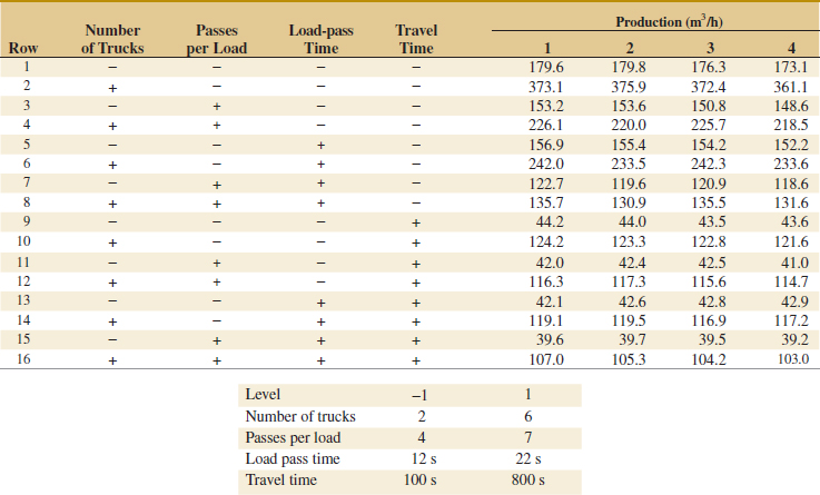
![]() 14-35. The book Using Designed Experiments to Shrink Health Care Costs [1997, ASQ Quality Press] presented a case study of an unreplicated 25 factorial design to investigate the effect of five factors on the length of accounts receivable measured in days. A summary of the investigated factors and the results of the study follows.
14-35. The book Using Designed Experiments to Shrink Health Care Costs [1997, ASQ Quality Press] presented a case study of an unreplicated 25 factorial design to investigate the effect of five factors on the length of accounts receivable measured in days. A summary of the investigated factors and the results of the study follows.
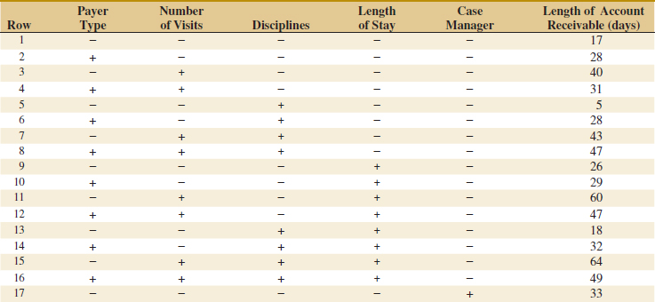
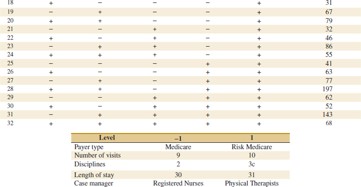
(a) Construct the normal probability plot of the effects and interpret the plot.
(b) Pool the negligible higher-order interactions to obtain an estimate of the error and construct the ANOVA accordingly.
(c) Analyze the residuals and comment on model adequacy.
14-6 Blocking and Confounding in the 2k Design
Running all the observations in a 2k factorial design under homogeneous conditions is often impossible. Blocking is the appropriate design technique for this general situation. However, in many situations, the block size is smaller than the number of runs in the complete replicate. In these cases, confounding is a useful procedure for running the 2k design in 2p blocks where the number of runs in a block is less than the number of treatment combinations in one complete replicate. The technique causes certain interaction effects to be indistinguishable from blocks or confounded with blocks. We illustrate confounding in the 2k factorial design in 2p blocks where p < k.
Consider a 22 design. Suppose that each of the 22 = 4 treatment combinations requires four hours of laboratory analysis. Thus, two days are required to perform the experiment. If days are considered as blocks, we must assign two of the four treatment combinations to each day.
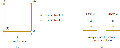
FIGURE 14-28 A 22 design in two blocks. (a) Geometric view. (b) Assignment of the four runs to two blocks.
See this design in Fig. 14-28. Notice that block 1 contains the treatment combinations (1) and ab and that block 2 contains a and b. The contrasts for estimating the main effects of factors A and B are
![]()
Note that these contrasts are unaffected by blocking because in each contrast there is one plus and one minus treatment combination from each block. That is, any difference between block 1 and block 2 that increases the readings in one block by an additive constant cancels out. The contrast for the AB interaction is
![]()
Because the two treatment combinations with the plus signs, ab and (1), are in block 1 and the two with the minus signs, a and b, are in block 2, the block effect and the AB interaction are identical. That is, the AB interaction is confounded with blocks.
The reason for this is apparent from the table of plus and minus signs for the 22 design in Table 14-12. From the table, we see that all treatment combinations that have a plus on AB are assigned to block 1 whereas all treatment combinations that have a minus sign on AB are assigned to block 2.
This scheme can be used to confound any 2k design in two blocks. As a second example, consider a 23 design, run in two blocks. From the table of plus and minus signs in Table 14-15, we assign the treatment combinations that are minus in the ABC column to block 1 and those that are plus in the ABC column to block 2. The resulting design is shown in Fig. 14-29.
There is a more general method of constructing the blocks. The method employs a defining contrast, say,
![]()
where xi is the level of the ith factor appearing in a treatment combination and αi is the exponent appearing on the ith factor in the effect that is to be confounded with blocks. For the 2k system, we have either αi = 0 or 1, and either xi = 0 (low level) or xi = 1 (high level). Treatment combinations that produce the same value of L (modulus 2) are placed in the same block. Because the only possible values of L (mod 2) are 0 and 1, this assigns the 2k treatment combinations to exactly two blocks.
As an example, consider the 23 design with ABC confounded with blocks. Here x1 corresponds to A, x2 to B, x3 to C, and α1 = α2 = α3 = 1. Thus, the defining contrast that would be used to confound ABC with blocks is
![]()
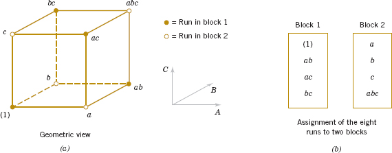
FIGURE 14-29 The 23 design in two blocks with ABC confounded. (a) Geometric view. (b) Assignment of the eight runs to two blocks.
To assign the treatment combinations to the two blocks, we substitute the treatment combinations into the defining contrast as follows:
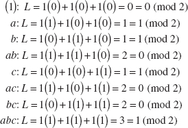
Thus (1), ab, ac, and bc are run in block 1, and a, b, c, and abc are run in block 2. This same design is shown in Fig. 14-29.
A shortcut method is useful in constructing these designs. The block containing the treatment combination (1) is called the principal block. Any element [except (1)] in the principal block may be generated by multiplying two other elements in the principal block modulus 2 on the exponents. For example, consider the principal block of the 23 design with ABC confounded, shown in Fig. 14-29. Note that
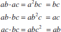
Treatment combinations in the other block (or blocks) may be generated by multiplying one element in the new block by each element in the principal block modulus 2 on the exponents. For the 23 with ABC confounded, because the principal block is (1), ab, ac, and bc, we know that the treatment combination b is in the other block. Thus, elements of this second block are
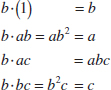
Example 14-7 Missile Miss Distance An experiment is performed to investigate the effect of four factors on the terminal miss distance of a shoulder-fired ground-to-air missile. The four factors are target type (A), seeker type (B), target altitude (C), and target range (D). Each factor may be conveniently run at two levels, and the optical tracking system allows terminal miss distance to be measured to the nearest foot. Two different operators or gunners are used in the flight test and, because there may be differences between operators, the test engineers decided to conduct the 24 design in two blocks with ABCD confounded. Thus, the defining contrast is
![]()
The experimental design and the resulting data are shown in Fig. 14-30. The effect estimates obtained from computer software are shown in Table 14-23. A normal probability plot of the effects in Fig. 14-31 reveals that A (target type), D (target range), AD, and AC have large effects. A confirming analysis, pooling the three-factor interactions as error, is shown in Table 14-24.
Practical Interpretation: Because the AC and AD interactions are significant, it is logical to conclude that A (target type), C (target altitude), and D (target range) all have important effects on the miss distance and that there are interactions between target type and altitude and target type and range. Notice that the ABCD effect is treated as blocks in this analysis.
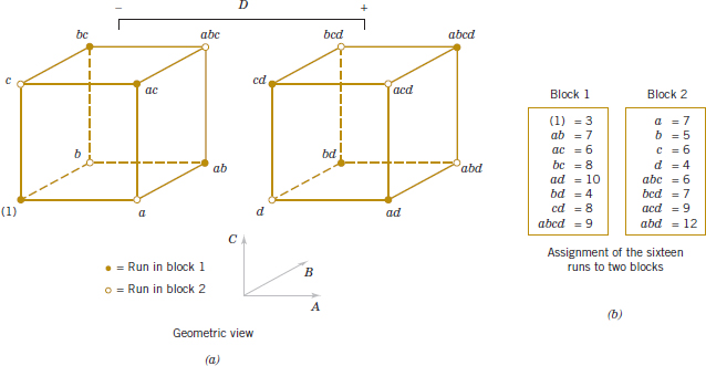
FIGURE 14-30 The 24 design in two blocks for example 14-7. (a) Geometric view. (b) Assignment of the 16 runs to two blocks.
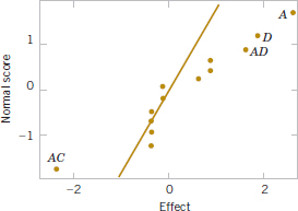
FIGURE 14-31 Normal probability plot of the effects for the Missile Miss Distance Experiment.
![]() TABLE • 14-23 Effect Estimates from Computer Output for the Missile Miss Distance Experiment in Example 14-7
TABLE • 14-23 Effect Estimates from Computer Output for the Missile Miss Distance Experiment in Example 14-7
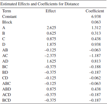
It is possible to confound the 2k design in four blocks of 2k−2 observations each. To construct the design, two effects are chosen to confound with blocks, and their defining contrasts are obtained. A third effect, the generalized interaction of the two effects initially chosen, is also confounded with blocks. The generalized interaction of two effects is found by multiplying their respective letters and reducing the exponents modulus 2.
![]() TABLE • 14-24 Analysis for the Missile Miss Distance Experiment
TABLE • 14-24 Analysis for the Missile Miss Distance Experiment
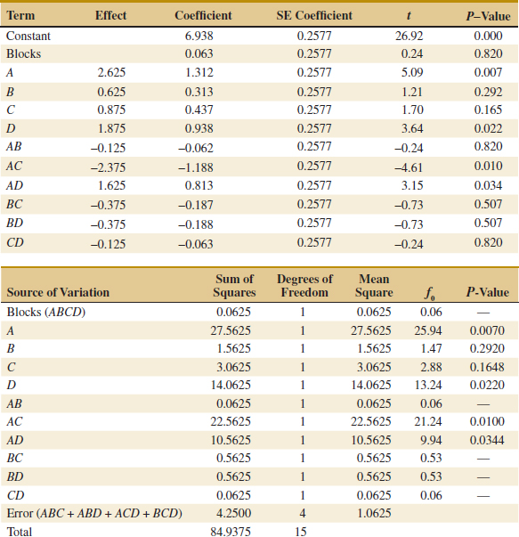
For example, consider the 24 design in four blocks. If AC and BD are confounded with blocks, their generalized interaction is (AC)(BD) = ABCD. The design is constructed by using the defining contrasts for AC and BD:
![]()
It is easy to verify that the four blocks are
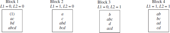
This general procedure can be extended to confounding the 2k design in 2p blocks where p < k. Start by selecting p effects to be confounded such that no effect chosen is a generalized interaction of the others. Then the blocks can be constructed from the p defining contrasts L1, L2,..., Lp that are associated with these effects. In addition to the p effects chosen to be confounded, exactly 2p − p − 1 additional effects are confounded with blocks; these are the generalized interactions of the original p effects chosen. Care should be taken so as not to confound effects of potential interest.
For more information on confounding in the 2k factorial design, refer to Montgomery (2012) for guidelines on selecting factors to confound with blocks so that main effects and low-order interactions are not confounded. In particular, that book has a table of suggested confounding schemes for designs with up to seven factors and a range of block sizes, some of which are as small as two runs.
Exercises FOR SECTION 14-6
![]() Problem available in WileyPLUS at instructor's discretion.
Problem available in WileyPLUS at instructor's discretion.
![]() Go Tutorial Tutoring problem available in WileyPLUS at instructor's discretion.
Go Tutorial Tutoring problem available in WileyPLUS at instructor's discretion.
![]() 14-36.
14-36. ![]() Consider the data from the first replicate of Exercise 14-14.
Consider the data from the first replicate of Exercise 14-14.
(a) Suppose that these observations could not all be run under the same conditions. Set up a design to run these observations in two blocks of four observations each with ABC confounded.
(b) Analyze the data.
![]() 14-37. Consider the data from the first replicate of Exercise 14-15.
14-37. Consider the data from the first replicate of Exercise 14-15.
(a) Construct a design with two blocks of eight observations each with ABCD confounded.
(b) Analyze the data.
![]() 14-38. Consider the data from Exercise 14-20.
14-38. Consider the data from Exercise 14-20.
(a) Construct the design that would have been used to run this experiment in two blocks of eight runs each.
(b) Analyze the data and draw conclusions.
14-39. Construct a 25 design in two blocks. Select the ABCDE interaction to be confounded with blocks.
![]() 14-40. Consider the data from the first replicate of Exercise 14-15, assuming that four blocks are required. Confound ABD and ABC (and consequently CD) with blocks.
14-40. Consider the data from the first replicate of Exercise 14-15, assuming that four blocks are required. Confound ABD and ABC (and consequently CD) with blocks.
(a) Construct a design with four blocks of four observations each.
(b) Analyze the data.
14-41. ![]() Construct a 25 design in four blocks. Select the appropriate effects to confound so that the highest possible interactions are confounded with blocks.
Construct a 25 design in four blocks. Select the appropriate effects to confound so that the highest possible interactions are confounded with blocks.
14-42. Consider the 26 factorial design. Set up a design to be run in four blocks of 16 runs each. Show that a design that confounds three of the four-factor interactions with blocks is the best possible blocking arrangement.
![]() 14-43. An article in Quality Engineering [“Designed Experiment to Stabilize Blood Glucose Levels” (1999–2000, Vol. 12, pp. 83–87)] reported on an experiment to minimize variations in blood glucose levels. The factors were volume of juice intake before exercise (4 or 8 oz), amount of exercise on a Nordic Track cross-country skier (10 or 20 min), and delay between the time of juice intake (0 or 20 min) and the beginning of the exercise period. The experiment was blocked for time of day. The data follow.
14-43. An article in Quality Engineering [“Designed Experiment to Stabilize Blood Glucose Levels” (1999–2000, Vol. 12, pp. 83–87)] reported on an experiment to minimize variations in blood glucose levels. The factors were volume of juice intake before exercise (4 or 8 oz), amount of exercise on a Nordic Track cross-country skier (10 or 20 min), and delay between the time of juice intake (0 or 20 min) and the beginning of the exercise period. The experiment was blocked for time of day. The data follow.
(a) What effects are confounded with blocks? Comment on any concerns with the confounding in this design.
(b) Analyze the data and draw conclusions.
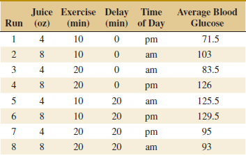
![]()
14-44. ![]() An article in Industrial and Engineering Chemistry [“Factorial Experiments in Pilot Plant Studies” (1951, pp. 1300–1306)] reports on an experiment to investigate the effect of temperature (A), gas throughput (B), and concentration (C) on the strength of product solution in a recirculation unit. Two blocks were used with ABC confounded, and the experiment was replicated twice. The data follow.
An article in Industrial and Engineering Chemistry [“Factorial Experiments in Pilot Plant Studies” (1951, pp. 1300–1306)] reports on an experiment to investigate the effect of temperature (A), gas throughput (B), and concentration (C) on the strength of product solution in a recirculation unit. Two blocks were used with ABC confounded, and the experiment was replicated twice. The data follow.
(a) Analyze the data from this experiment.
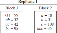
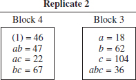
(b) Analyze the residuals and comment on model adequacy.
(c) Comment on the efficiency of this design. Note that we have replicated the experiment twice, yet we have no information on the ABC interaction.
(d) Suggest a better design, specifically one that would provide some information on all interactions.
14-45. Consider the following computer output from a single replicate of a 24 experiment in two blocks with ABCD confounded.
(a) Comment on the value of blocking in this experiment.
(b) What effects were used to generate the residual error in the ANOVA?
(c) Calculate the entries marked with “?” in the output.
Factorial Fit: y Versus Block, A, B, C, D
Estimated Effects and Coefficients
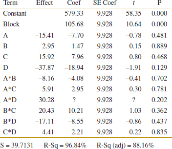
![]() 14-46. An article in Advanced Semiconductor Manufacturing Conference (ASMC) (May 2004, pp. 325–29) stated that dispatching rules and rework strategies are two major operational elements that impact productivity in a semiconductor fabrication plant (fab). A four-factor experiment was conducted to determine the effect of dispatching rule time (5 or 10 min), rework delay (0 or 15 min), fab temperature (60 or 80°F), and rework levels (level 0 or level 1) on key fab performance measures. The performance measure that was analyzed was the average cycle time. The experiment was blocked for the fab temperature. Data modified from the original study are in the following table.
14-46. An article in Advanced Semiconductor Manufacturing Conference (ASMC) (May 2004, pp. 325–29) stated that dispatching rules and rework strategies are two major operational elements that impact productivity in a semiconductor fabrication plant (fab). A four-factor experiment was conducted to determine the effect of dispatching rule time (5 or 10 min), rework delay (0 or 15 min), fab temperature (60 or 80°F), and rework levels (level 0 or level 1) on key fab performance measures. The performance measure that was analyzed was the average cycle time. The experiment was blocked for the fab temperature. Data modified from the original study are in the following table.
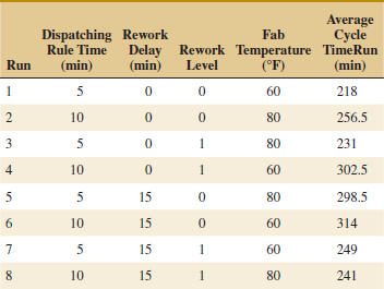
(a) What effects are confounded with blocks? Do you find any concerns with confounding in this design? If so, comment on it.
(b) Analyze the darta and draw conclusions.
![]()
14-47. Consider the earth-moving experiment in Exercise 14-34. The experiment actually used two different operators with the production in columns 1 and 3 from operator 1 and 2, respectively. Analyze the results from only columns 1 and 3 handled as blocks.
(a) Assuming that the operator is a nuisance factor, estimate the factor effects.
(b) Based on a normal probability plot of the effect estimates, identify a model for the data from this experiment.
(c) Conduct an ANOVA based on the model identified in part (a). What are the conclusions?
(d) Analyze the residuals and plot residuals versus the predicted production.
(e) Compare the results from this analysis to the previous analysis that did not use blocking.
![]()
14-48. An article in Journal of Hazardous Materials [“Biosorption of Reactive Dye Using Acid-Treated Rice Husk: Factorial Design Analysis” (2007, Vol. 142(1), pp. 397–403)] described an experiment using biosorption to remove red color from water. A 24 full factorial design was used to study the effect of factors pH, temperature, adsorbent dosage, and initial concentration of the dye. Handle columns 1 and 2 of the output as blocks.
(a) Estimate the factor effects. Based on a normal probability plot of the effect estimates, identify a model for the data from this experiment.
(b) Conduct an ANOVA based on the model identified in part (a). What are the conclusions?
(c) Analyze the residuals and plot residuals versus the predicted removal efficiency.
(d) Construct a regression model to predict removal efficiency in terms of the actual factor levels.
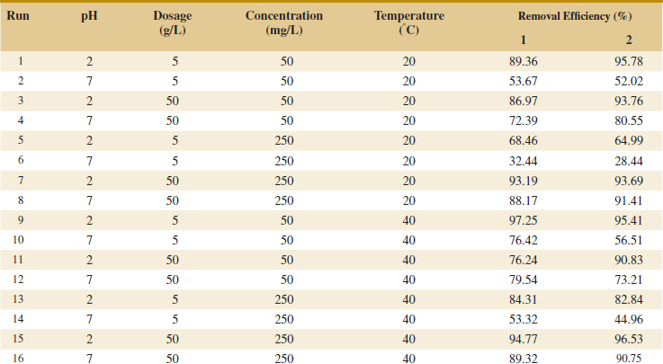
14-7 FRACTIONAL REPLICATION OF THE 2k DESIGN
As the number of factors in a 2k factorial design increases, the number of runs required increases rapidly. For example, a 25 requires 32 runs. In this design, only 5 degrees of freedom correspond to main effects, and 10 degrees of freedom correspond to two-factor interactions. Sixteen of the 31 degrees of freedom are used to estimate high-order interactions—that is, three-factor and higher order interactions. Often there is little interest in these high-order interactions, particularly when we first begin to study a process or system. If we can assume that certain high-order interactions are negligible, a fractional factorial design involving fewer than the complete set of 2k runs can be used to obtain information on the main effects and low-order interactions. In this section, we introduce fractional replications of the 2k design.
A major use of fractional factorials is in screening experiments. These are experiments in which many factors are considered with the purpose of identifying those factors (if any) that have large effects. Screening experiments are usually performed in the early stages of a project when it is likely that many of the factors initially considered have little or no effect on the response. The factors that are identified as important are then investigated more thoroughly in subsequent experiments.
14-7.1 ONE-HALF FRACTION OF THE 2k DESIGN
A one-half fraction of the 2k design contains 2k−1 runs and is often called a 2k−1 fractional factorial design. As an example, consider the 23−1 design—that is, a one-half fraction of the 23. This design has only four runs in contrast to the full factorial that would require eight runs. The table of plus and minus signs for the 23 design is shown in Table 14-25. Suppose that we select the four treatment combinations a, b, c, and abc as our one-half fraction. These treatment combinations are shown in the top half of Table 14-25 and in Fig. 14-32(a).
![]() TABLE • 14-25 Plus and Minus Signs for the 23 Factorial Design
TABLE • 14-25 Plus and Minus Signs for the 23 Factorial Design
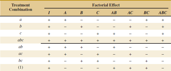
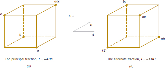
FIGURE 14-32 The one-half fractions of the 23 design. (a) The principal fraction, I = +ABC. (b) The alternate fraction, I = −ABC.
Notice that the 23−1 design is formed by selecting only those treatment combinations that yield a plus on the ABC effect. Thus, ABC is called the generator of this particular fraction. Furthermore, the identity element I is also plus for the four runs, so we call
![]()
the defining relation for the design.
The treatment combinations in the 23−1 design yields three degrees of freedom associated with the main effects. From the upper half of Table 14-25, we obtain the estimates of the main effects as linear combinations of the observations, say,
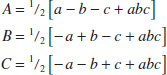
It is also easy to verify that the estimates of the two-factor interactions should be the following linear combinations of the observations:
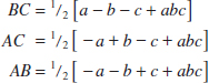
Thus, the linear combination of observations in column A, ℓA estimates both the main effect of A and the BC interaction. That is, the linear combination ℓA estimates the sum of these two effects A + BC. Similarly, ℓB estimates B + AC, and ℓC estimates C + AB. Two or more effects that have this property are called aliases. In our 23−1 design, A and BC are aliases, B and AC are aliases, and C and AB are aliases. Aliasing is the direct result of fractional replication. In many practical situations, it is possible to select the fraction so that the main effects and low-order interactions that are of interest are aliased only with high-order interactions (which are probably negligible).
The alias structure for this design is found by using the defining relation I = ABC. Multiplying any effect by the defining relation yields the aliases for that effect. In our example, the alias of A is
![]()
because A · I = A and A2 = I. The aliases of B and C are
![]()
Now suppose that we had chosen the other one-half fraction, that is, the treatment combinations in Table 14-25 associated with minus on ABC. See these four runs in the lower half of Table 14-25 and in Fig. 14-32(b). The defining relation for this design is I = −ABC. The aliases are A = −BC, B = −AC, and C = −AB. Thus, estimates of A, B, and C that result from this fraction really estimate A −BC, B −AC, and C −AB. In practice, it usually does not matter which one-half fraction we select. The fraction with the plus sign in the defining relation is usually called the principal fraction, and the other fraction is usually called the alternate fraction.
Note that if we had chosen AB as the generator for the fractional factorial A = A · AB = B and the two main effects of A and B would be aliased. This typically loses important information.
Sometimes we use sequences of fractional factorial designs to estimate effects. For example, suppose that we had run the principal fraction of the 23−1 design with generator ABC. From this design, we have the following effect estimates:
![]()
Suppose that we are willing at this point to assume that the two-factor interactions are negligible. If they are, the 23−1 design has produced estimates of the three main effects A, B, and C. However, if after running the principal fraction, we are uncertain about the interactions, it is possible to estimate them by running the alternate fraction. The alternate fraction produces the following effect estimates:
![]()
We may now obtain de-aliased estimates of the main effects and two-factor interactions by adding and subtracting the linear combinations of effects estimated in the two individual fractions. For example, suppose that we want to de-alias A from the two-factor interaction BC. Because ℓA = A + BC and ![]() = A − BC, we can combine these effect estimates as follows:
= A − BC, we can combine these effect estimates as follows:
![]()
and
![]()
For all three pairs of effect estimates, we would obtain the following results:
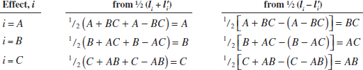
Thus, by combining a sequence of two fractional factorial designs, we can isolate both the main effects and the two-factor interactions. This property makes the fractional factorial design highly useful in experimental problems because we can run sequences of small, efficient experiments, combine information across several experiments, and take advantage of learning about the process we are experimenting with as we go along. This is an illustration of the concept of sequential experimentation.
A 2k−1 design may be constructed by writing down the treatment combinations for a full factorial with k − 1 factors, called the basic design, and then adding the kth factor by identifying its plus and minus levels with the plus and minus signs of the highest order interaction. Therefore, a 23−1 fractional factorial is constructed by writing down the basic design as a full 22 factorial and then equating factor C with the ±AB interaction. Thus, to construct the principal fraction, we would use C = +AB as follows:
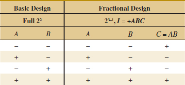
To obtain the alternate fraction, we would equate the last column to C = −AB.
Example 14-8 Plasma Etch To illustrate the use of a one-half fraction, consider the plasma etch experiment described in Example 14-5. Suppose that we decide to use a 24−1 design with I = ABCD to investigate the four factors gap (A), pressure (B), C2F6 flow rate (C), and power setting (D). This design would be constructed by writing as the basic design a 23 in the factors A, B, and C and then setting the levels of the fourth factor D = ABC. The design and the resulting etch rates are shown in Table 14-26. The design is shown graphically in Fig. 14-33.
In this design, the main effects are aliased with the three-factor interactions; note that the alias of A is
![]()
and similarly, B = ACD, C = ABD, and D = ABC.
The two-factor interactions are aliased with each other. For example, the alias of AB is CD:
![]()
![]() TABLE • 14-26 The 24−1 Design with Defining Relation I = ABCD
TABLE • 14-26 The 24−1 Design with Defining Relation I = ABCD
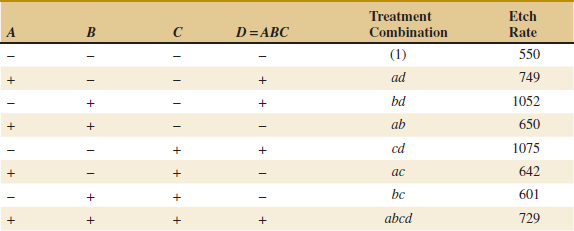
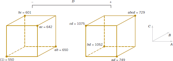
FIGURE 14-33 The 24−1 design for the plasma etch experiment of Example 14-8.
The other aliases are AC = BD and AD = BC.
The estimates of the main effects and their aliases are found using the four columns of signs in Table 14-26. For example, from column A, we obtain the estimated effect
![]()
The other columns produce
![]()
and
![]()
Clearly, ℓA and ℓD are large, and if we believe that the three-factor interactions are negligible, the main effects A (gap) and D (power setting) significantly affect etch rate.
The interactions are estimated by forming the AB, AC, and AD columns and adding them to the table. For example, the signs in the AB column are +, −, −, +, +, −, −, +, and this column produces the estimate
![]()
From the AC and AD columns we find
![]()
and
![]()
The ℓAD estimate is large; the most straightforward interpretation of the results is that because A and D are large, this is the AD interaction. Thus, the results obtained from the 24−1 design agree with the full factorial results in Example 14-5.
Practical Interpretation: Often a fraction of a 2k design is satisfactory when an experiment uses four or more factors.
Computer Solution
Fractional factorial designs are usually analyzed with a software package. Table 14-27 shows the effect estimates obtained from computer software for the plasma etch experiment in Example 14-8. They are in agreement with the hand calculation reported earlier.
Normal Probability Plot of Effects
The normal probability plot is very useful in assessing the significance of effects from a fractional factorial design, particularly when many effects are to be estimated. We strongly recommend examining this plot. Figure 14-34 presents the normal probability plot of the effects from computer software for the plasma etch experiment in Example 14-8. Notice that the A, D, and AD interaction effects stand out clearly in this graph.
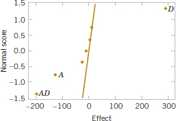
FIGURE 14-34 Normal probability plot of the effects for the plasma etch experiment in Example 14-8.
![]() TABLE • 14-27 Effect Estimates from Computer Software for the Plasma Etch Experiment in Example 14-8
TABLE • 14-27 Effect Estimates from Computer Software for the Plasma Etch Experiment in Example 14-8
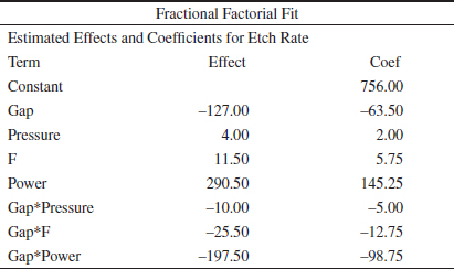
Residual Analysis
The residuals can be obtained from a fractional factorial by the regression model method shown previously. Note that the computer output for Example 14-8 in Table 14-27 shows the regression coefficients. The residuals should be graphically analyzed as we have discussed before, both to assess the validity of the underlying model assumptions and to gain additional insight into the experimental situation.
Center Points
Center points can be added to fractional factorial designs for the same reasons as before; that is, to assess curvature and provide an error estimate. The curvature analysis compares ![]() F −
F − ![]() C to its standard error with the same calculation as for full factorial experiments. The error estimate can be based on the replicated center points and supplemented with sums of squares from effects determined to be unimportant from the normal probability plot.
C to its standard error with the same calculation as for full factorial experiments. The error estimate can be based on the replicated center points and supplemented with sums of squares from effects determined to be unimportant from the normal probability plot.
Projection of the 2k−1 Design
If one or more factors from a one-half fraction of a 2k can be dropped, the design projects into a full factorial design. For example, Fig. 14-35 presents a 23−1 design. Notice that this design projects into a full factorial in any two of the three original factors. Thus, if we think that at most two of the three factors are important, the 23−1 design is an excellent design for identifying the significant factors. This projection property is highly useful in factor screening because it allows negligible factors to be eliminated, resulting in a stronger experiment in the active factors that remain.
In the 24−1 design used in the plasma etch experiment in Example 14-8, we found that two of the four factors (B and C) could be dropped. If we eliminate these two factors, the remaining columns in Table 14-26 form a 22 design in the factors A and D with two replicates. This design is shown in Fig. 14-36. The main effects of A and D and the strong two-factor AD interaction are clearly evident from this graph.
Design Resolution
The concept of design resolution is a useful way to catalog fractional factorial designs according to the alias patterns they produce. Designs of resolution III, IV, and V are particularly important. The definitions of these terms and an example of each follow.
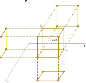
FIGURE 14-35 Projection of a 23−1 design into three 22 designs.
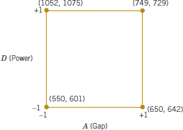
FIGURE 14-36 The 22 design obtained by dropping factors B and C from the plasma etch experiment in Example 14-8.
- Resolution III Designs. These are designs in which no main effects are aliased with any other main effect, but main effects are aliased with two-factor interactions, and some two-factor interactions may be aliased with each other. The 23−1 design with I = ABC is a resolution III design. We usually employ a Roman numeral subscript to indicate design resolution; thus, this one-half fraction is a
 design.
 - Resolution IV Designs. These are designs in which no main effect is aliased with any other main effect or two-factor interactions, but two-factor interactions are aliased with each other. The 24−1 design with I = ABCD used in Example 14-8 is a resolution IV design
 .
. - Resolution V Designs. These are designs in which no main effect or two-factor interaction is aliased with any other main effect or two-factor interaction, but two-factor interactions are aliased with three-factor interactions. The 25−1 design with I = ABCDE is a resolution V design
 .
.
Resolution III and IV designs are particularly useful in factor screening experiments. A resolution IV design provides good information about main effects and some information about all two-factor interactions.
14-7.2 SMALLER FRACTIONS: THE 2k−p FRACTIONAL FACTORIAL
Although the 2k−1 design is valuable in reducing the number of runs required for an experiment, we frequently find that smaller fractions provide almost as much useful information at even greater economy. In general, a 2k design may be run in a 1/2p fraction called a 2k−p fractional factorial design. Thus, a 1/4 fraction is called a 2k−2 design, a 1/8 fraction is called a 2k−3 design, a 1/16 fraction a 2k−4 design, and so on.
To illustrate the 1/4 fraction, consider an experiment with six factors and suppose that the engineer is primarily interested in main effects but would also like to get some information about the two-factor interactions. A 26−1 design would require 32 runs and would have 31 degrees of freedom for estimating effects. Because there are only six main effects and 15 two-factor interactions, the one-half fraction is inefficient—it requires too many runs. Suppose that we consider a 1/4 fraction, or a 26−2 design. This design contains 16 runs and, with 15 degrees of freedom, allows all six main effects to be estimated with some capability for examining the two-factor interactions.
To generate this design, we would write down a 24 design in the factors A, B, C, and D as the basic design and then add two columns, for E and F. To find the new columns, we could select the two design generators I = ABCE and I = BCDF. Thus, column E would be found from E = ABC, and column F would be F = BCD. That is, columns ABCE and BCDF are equal to the identity column. However, we know that the product of any two columns in the table of plus and minus signs for a 2k design is just another column in the table; therefore, the product of ABCE and BCDF or ABCE(BCDF) = AB2C2DEF = ADEF is also an identity column. Consequently, the complete defining relation for the 26−2 design is
![]()
We refer to each term in a defining relation (such as ABCE above) as a word. To find the alias of any effect, simply multiply the effect by each word in the foregoing defining relation. For example, the alias of A is
![]()
The complete alias relationships for this design are in Table 14-28. In general, the resolution of a 2k−p design is equal to the number of letters in the shortest word in the complete defining relation. Therefore, this is a resolution IV design; main effects are aliased with three-factor and higher interactions, and two-factor interactions are aliased with each other. This design would provide good information on the main effects and would give some idea about the strength of the two-factor interactions. The construction and analysis of the design are illustrated in Example 14-9.
![]() TABLE • 14-28 Alias Structure for the
TABLE • 14-28 Alias Structure for the ![]() Design with I = ABCE = BCDF = ADEF
Design with I = ABCE = BCDF = ADEF
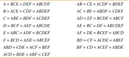
Example 14-9 Injection Molding Parts manufactured in an injection-molding process are showing excessive shrinkage, which is causing problems in assembly operations upstream from the injection-molding area. In an effort to reduce the shrinkage, a quality-improvement team has decided to use a designed experiment to study the injection-molding process. The team investigates each of six factors—mold temperature (A), screw speed (B), holding time (C), cycle time (D), gate size (E), and holding pressure (F)—at two levels with the objective of learning how each factor affects shrinkage and obtaining preliminary information about how the factors interact.
The team decides to use a 16-run two-level fractional factorial design for these six factors. The design is constructed by writing a 24 as the basic design in the factors A, B, C, and D and then setting E = ABC and F = BCD as discussed previously. Table 14-29 shows the design along with the observed shrinkage (× 10) for the test part produced at each of the 16 runs in the design.
A normal probability plot of the effect estimates from this experiment is shown in Fig. 14-37. The only large effects are A (mold temperature), B (screw speed), and the AB interaction. In light of the alias relationship in Table 14-28, it seems reasonable to tentatively adopt these conclusions. The plot of the AB interaction in Fig. 14-38 shows that the process is insensitive to temperature if the screw speed is at the low level but sensitive to temperature if the screw speed is at the high level. With the screw speed at a low level, the process should produce an average shrinkage of around 10% regardless of the temperature level chosen.
![]() TABLE • 14-29 A
TABLE • 14-29 A ![]() Design for the Injection-Molding Experiment
Design for the Injection-Molding Experiment
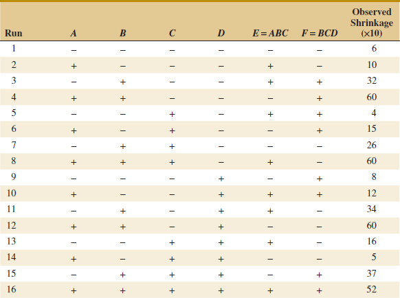
Based on this initial analysis, the team decides to set both the mold temperature and the screw speed at the low level. This set of conditions should reduce the mean shrinkage of parts to around 10%. However, the variability in shrinkage from part to part is still a potential problem. In effect, the mean shrinkage can be adequately reduced by the preceding modifications; however, the part-to-part variability in shrinkage over a production run could still cause problems in assembly. One way to address this issue is to see whether any of the process factors affect the variability in parts shrinkage.
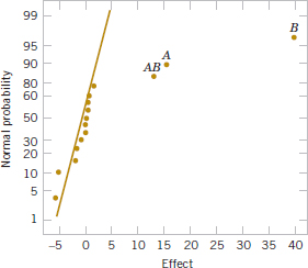
FIGURE 14-37 Normal probability plot of effects for the injection-molding experiment in Example 14-9.
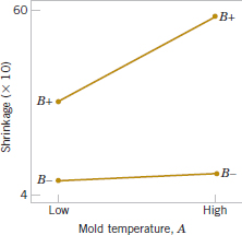
FIGURE 14-38 Plot of AB (mold temperature–screw speed) interaction for the injection-molding experiment in Example 14-9.
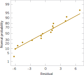
FIGURE 14-39 Normal probability plot of residuals for the injection-molding experiment in Example 14-9.

FIGURE 14-40 Residuals versus holding time (C) for the injection-molding experiment in Example 14-9.
Figure 14-39 presents the normal probability plot of the residuals. This plot appears satisfactory. The plots of residuals versus each factor were then constructed. One of these plots, that for residuals versus factor C (holding time), is shown in Fig. 14-40. The plot reveals much less scatter in the residuals at the low holding time than at the high holding time. These residuals were obtained in the usual way from a model for predicted shrinkage
![]()
where x1, x2, and x1x2 are coded variables that correspond to the factors A and B and the AB interaction. The regression model used to produce the residuals essentially removes the location effects of A, B, and AB from the data; the residuals therefore contain information about unexplained variability. Figure 14-40 indicates that there is a pattern in the variability and that the variability in the shrinkage of parts may be smaller when the holding time is at the low level.
Practical Interpretation: Figure 14-41 shows the data from this experiment projected onto a cube in the factors A, B, and C. The average observed shrinkage and the range of observed shrinkage are shown at each corner of the cube. From inspection of this figure, we see that running the process with the screw speed (B) at the low level is the key to reducing average parts shrinkage. If B is low, virtually any combination of temperature (A) and holding time (C) results in low values of average parts shrinkage. However, from examining the ranges of the shrinkage values at each corner of the cube, it is immediately clear that setting the holding time (C) at the low level is the most appropriate choice if we wish to keep the part-to-part variability in shrinkage low during a production run.
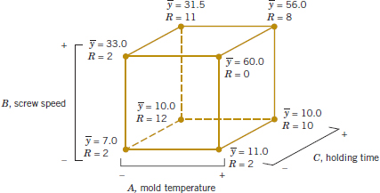
FIGURE 14-41 Average shrinkage and range of shrinkage in factors A, B, and C for Example 14-9.
The concepts used in constructing the 26−2 fractional factorial design in Example 14-9 can be extended to the construction of any 2k−p fractional factorial design. In general, a 2k fractional factorial design containing 2k−p runs is called a 1/2p fraction of the 2k design or, more simply, a 2k−p fractional factorial design. These designs require the selection of p independent generators. The defining relation for the design consists of the p generators initially chosen and their 2p − p − 1 generalized interactions.
The alias structure may be found by multiplying each effect column by the defining relation. Care should be exercised in choosing the generators so that effects of potential interest are not aliased with each other. Each effect has 2p − 1 aliases. For moderately large values of k, we usually assume that higher order interactions (say, third- or fourth-order or higher) to be negligible, and this greatly simplifies the alias structure.
It is important to select the p generators for the 2k−p fractional factorial design in such a way that we obtain the best possible alias relationships. A reasonable criterion is to select the generators so that the resulting 2k−p design has the highest possible design resolution. Montgomery (2012) presented a table of recommended generators for 2k−p fractional factorial designs for k ≤ 15 factors and up to as many as n ≤ 128 runs. A portion of his table is reproduced here as Table 14-30. In this table, the generators are shown with either + or − choices; selection of all generators as + provides a principal fraction, and if any generators are − choices, the design is one of the alternate fractions for the same family. The suggested generators in this table produce a design of the highest possible resolution. Montgomery (2012) also provided a table of alias relationships for these designs.
![]() TABLE • 14-30 Selected 2k−p Fractional Factorial Designs
TABLE • 14-30 Selected 2k−p Fractional Factorial Designs
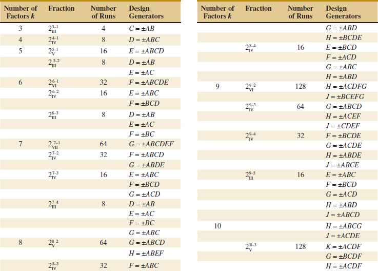
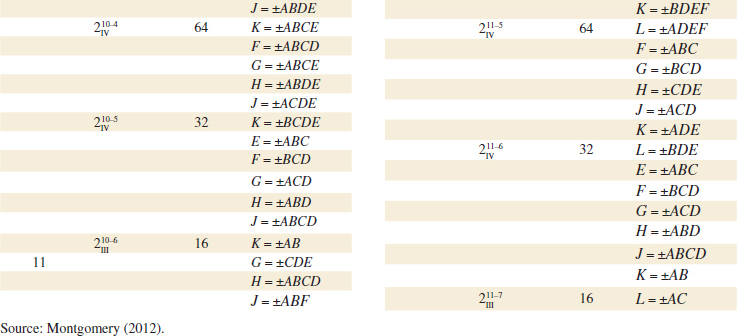
Example 14-10 Aliases with Seven Factors To illustrate the use of Table 14-30, suppose that we have seven factors and that we are interested in estimating the seven main effects and obtaining some insight regarding the two-factor interactions. We are willing to assume that three-factor and higher interactions are negligible. This information suggests that a resolution IV design is appropriate.
Table 14-30 shows that two resolution IV fractions are available: the ![]() with 32 runs and the
with 32 runs and the ![]() with 16 runs. The aliases involving main effects and two- and three-factor interactions for the 16-run design are presented in Table 14-31. Notice that all seven main effects are aliased with three-factor interactions. All the two-factor interactions are aliased in groups of three. Therefore, this design will satisfy our objectives; that is, it will allow the estimation of the main effects, and it will give some insight regarding two-factor interactions. It is not necessary to run the
with 16 runs. The aliases involving main effects and two- and three-factor interactions for the 16-run design are presented in Table 14-31. Notice that all seven main effects are aliased with three-factor interactions. All the two-factor interactions are aliased in groups of three. Therefore, this design will satisfy our objectives; that is, it will allow the estimation of the main effects, and it will give some insight regarding two-factor interactions. It is not necessary to run the ![]() design, which would require 32 runs. The construction of the
design, which would require 32 runs. The construction of the ![]() design is shown in Table 14-32. Notice that it was constructed by starting with the 16-run 24 design in A, B, C, and D as the basic design and then adding the three columns E = ABC, F = BCD, and G = ACD as suggested in Table 14-30. Thus, the generators for this design are I = ABCE, I = BCDF, and I = ACDG. The complete defining relation is I = ABCE = BCDF = ADEF = ACDG = BDEG = CEFG = ABFG. This defining relation was used to produce the aliases in Table 14-31. For example, the alias relationship of A is
design is shown in Table 14-32. Notice that it was constructed by starting with the 16-run 24 design in A, B, C, and D as the basic design and then adding the three columns E = ABC, F = BCD, and G = ACD as suggested in Table 14-30. Thus, the generators for this design are I = ABCE, I = BCDF, and I = ACDG. The complete defining relation is I = ABCE = BCDF = ADEF = ACDG = BDEG = CEFG = ABFG. This defining relation was used to produce the aliases in Table 14-31. For example, the alias relationship of A is
![]() TABLE • 14-31 Generators, Defining Relation, and Aliases for the
TABLE • 14-31 Generators, Defining Relation, and Aliases for the ![]() Fractional Factorial Design
Fractional Factorial Design
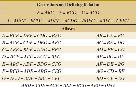
![]()
which, if we ignore interactions higher than three factors, agrees with Table 14-31.
![]() TABLE • 14-32 A
TABLE • 14-32 A ![]() Fractional Factorial Design
Fractional Factorial Design
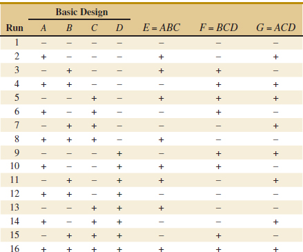
For seven factors, we can reduce the number of runs even further. The 27−4 design is an eight-run experiment accommodating seven variables. This is a 1/16th fraction that is obtained by first writing a 23 design as the basic design in the factors A, B, and C, and then forming the four new columns from I = ABD, I = ACE, I = BCF, and I = ABCG, as suggested in Table 14-30. The design is shown in Table 14-33.
The complete defining relation is found by multiplying the generators together two, three, and finally four at a time, producing
![]()
The alias of any main effect is found by multiplying that effect through each term in the defining relation. For example, the alias of A is
![]()
![]() TABLE • 14-33 A
TABLE • 14-33 A ![]() Fractional Factorial Design
Fractional Factorial Design
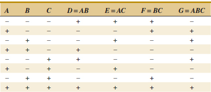
This design is of resolution III, because the main effect is aliased with two-factor interactions. If we assume that all three-factor and higher interactions are negligible, the aliases of the seven main effects are
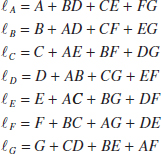
This ![]() design is called a saturated fractional factorial because all the available degrees of freedom are used to estimate main effects. It is possible to combine sequences of these resolution III fractional factorials to separate the main effects from the two-factor interactions. The procedure is illustrated in Montgomery (2012) and in Box, Hunter, and Hunter (2005).
design is called a saturated fractional factorial because all the available degrees of freedom are used to estimate main effects. It is possible to combine sequences of these resolution III fractional factorials to separate the main effects from the two-factor interactions. The procedure is illustrated in Montgomery (2012) and in Box, Hunter, and Hunter (2005).
Exercises FOR SECTION 14-7
![]() Problem available in WileyPLUS at instructor's discretion.
Problem available in WileyPLUS at instructor's discretion.
![]() Go Tutorial Tutoring problem available in WileyPLUS at instructor's discretion.
Go Tutorial Tutoring problem available in WileyPLUS at instructor's discretion.
![]() 14-49.
14-49. ![]() Consider the problem in Exercise 14-19. Suppose that only half of the 32 runs could be made.
Consider the problem in Exercise 14-19. Suppose that only half of the 32 runs could be made.
(a) Choose the half that you think should be run.
(b) Write out the alias relationships for your design.
(c) Estimate the factor effects.
(d) Plot the effect estimates on normal probability paper and interpret the results.
(e) Set up an analysis of variance for the factors identified as potentially interesting from the normal probability plot in part (d).
(f) Analyze the residuals from the model.
(g) Provide a practical interpretation of the results.
14-50. ![]() Suppose that in Exercise 14-22 it was possible to run only a
Suppose that in Exercise 14-22 it was possible to run only a ![]() fraction of the 24 design. Construct the design and use only the data from the eight runs you have generated to perform the analysis.
fraction of the 24 design. Construct the design and use only the data from the eight runs you have generated to perform the analysis.
![]()
14-51. ![]() An article by L. B. Hare [“In the Soup: A Case Study to Identify Contributors to Filling Variability,” Journal of Quality Technology 1988 (Vol. 20, pp. 36–43)] described a factorial experiment used to study filling variability of dry soup mix packages. The factors are A = number of mixing ports through which the vegetable oil was added (1, 2), B = temperature surrounding the mixer (cooled, ambient), C = mixing time (60, 80 sec), D = batch weight (1500, 2000 lb), and E = number of days of delay between mixing and packaging (1, 7). Between 125 and 150 packages of soup were sampled over an eight-hour period for each run in the design, and the standard deviation of package weight was used as the response variable. The design and resulting data follow.
An article by L. B. Hare [“In the Soup: A Case Study to Identify Contributors to Filling Variability,” Journal of Quality Technology 1988 (Vol. 20, pp. 36–43)] described a factorial experiment used to study filling variability of dry soup mix packages. The factors are A = number of mixing ports through which the vegetable oil was added (1, 2), B = temperature surrounding the mixer (cooled, ambient), C = mixing time (60, 80 sec), D = batch weight (1500, 2000 lb), and E = number of days of delay between mixing and packaging (1, 7). Between 125 and 150 packages of soup were sampled over an eight-hour period for each run in the design, and the standard deviation of package weight was used as the response variable. The design and resulting data follow.
(a) What is the generator for this design?
(b) What is the resolution of this design?
(c) Estimate the factor effects. Which effects are large?
(d) Does a residual analysis indicate any problems with the underlying assumptions?
(e) Draw conclusions about this filling process.
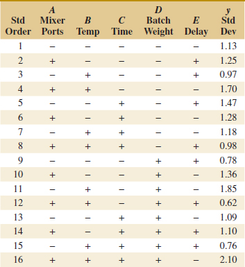
![]() 14-52.
14-52. ![]() Montgomery (2012) described a 24−1 fractional factorial design used to study four factors in a chemical process. The factors are A = temperature, B = pressure, C = concentration, and D = stirring rate, and the response is filtration rate. The design and the data are as follows:
Montgomery (2012) described a 24−1 fractional factorial design used to study four factors in a chemical process. The factors are A = temperature, B = pressure, C = concentration, and D = stirring rate, and the response is filtration rate. The design and the data are as follows:
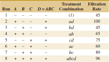
(a) Write down the alias relationships.
(b) Estimate the factor effects. Which factor effects appear large?
(c) Project this design into a full factorial in the three apparently important factors and provide a practical interpretation of the results.
![]() 14-53.
14-53. ![]() R. D. Snee (“Experimenting with a Large Number of Variables,” in Experiments in Industry: Design, Analysis and Interpretation of Results, Snee, Hare, and Trout, eds., ASQC, 1985) described an experiment in which a 25−1 design with I = ABCDE was used to investigate the effects of five factors on the color of a chemical product. The factors are A = solvent/reactant, B = catalyst/reactant, C = temperature, D = reactant purity, and E = reactant pH. The results obtained are as follows:
R. D. Snee (“Experimenting with a Large Number of Variables,” in Experiments in Industry: Design, Analysis and Interpretation of Results, Snee, Hare, and Trout, eds., ASQC, 1985) described an experiment in which a 25−1 design with I = ABCDE was used to investigate the effects of five factors on the color of a chemical product. The factors are A = solvent/reactant, B = catalyst/reactant, C = temperature, D = reactant purity, and E = reactant pH. The results obtained are as follows:
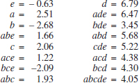
(a) Prepare a normal probability plot of the effects. Which factors are active?
(b) Calculate the residuals. Construct a normal probability plot of the residuals and plot the residuals versus the fitted values. Comment on the plots.
(c) If any factors are negligible, collapse the 25−1 design into a full factorial in the active factors. Comment on the resulting design, and interpret the results.
![]()
14-54. An article in Quality Engineering [“A Comparison of Multi-Response Optimization: Sensitivity to Parameter Selection” (1999, Vol. 11, pp. 405–415)] conducted a half replicate of a 25 factorial design to optimize the retort process of beef stew MREs, a military ration. The design factors are x1 = sauce viscosity, x2 = residual gas, x3 = solid/liquid ratio, x4 = net weight, x5 = rotation speed. The response variable is the heating rate index, a measure of heat penetration, and there are two replicates.
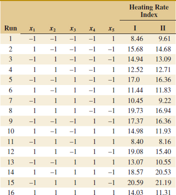
(a) Estimate the factor effects. Based on a normal probability plot of the effect estimates, identify a model for the data from this experiment.
(b) Conduct an ANOVA based on the model identified in part (a). What are your conclusions?
(c) Analyze the residuals and comment on model adequacy.
(d) Find a regression model to predict yield in terms of the coded factor levels.
(e) This experiment was replicated, so an ANOVA could have been conducted without using a normal plot of the effects to tentatively identify a model. What model would be appropriate? Use the ANOVA to analyze this model and compare the results with those obtained from the normal probability plot approach.
![]() 14-55.
14-55. ![]() An article in Industrial and Engineering Chemistry [“More on Planning Experiments to Increase Research Efficiency” (1970, pp. 60–65)] uses a 25−2 design to investigate the effect on process yield of A = condensation temperature, B = amount of material 1, C = solvent volume, D = condensation time, and E = amount of material 2. The results obtained are as follows:
An article in Industrial and Engineering Chemistry [“More on Planning Experiments to Increase Research Efficiency” (1970, pp. 60–65)] uses a 25−2 design to investigate the effect on process yield of A = condensation temperature, B = amount of material 1, C = solvent volume, D = condensation time, and E = amount of material 2. The results obtained are as follows:
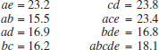
(a) Verify that the design generators used were I = ACE and I = BDE.
(b) Write down the complete defining relation and the aliases from the design.
(c) Estimate the main effects.
(d) Prepare an analysis of variance table. Verify that the AB and AD interactions are available to use as error.
(e) Plot the residuals versus the fitted values. Also construct a normal probability plot of the residuals. Comment on the results.
![]() 14-56.
14-56. ![]() Suppose that in Exercise 14-16 only a ¼ fraction of the 25 design could be run. Construct the design and analyze the data that are obtained by selecting only the response for the eight runs in your design.
Suppose that in Exercise 14-16 only a ¼ fraction of the 25 design could be run. Construct the design and analyze the data that are obtained by selecting only the response for the eight runs in your design.
14-57. ![]() For each of the following designs, write down the aliases, assuming that only main effects and two factor interactions are of interest.
For each of the following designs, write down the aliases, assuming that only main effects and two factor interactions are of interest.
(a) ![]()
(b) ![]()
14-58. ![]() Consider the 26−2 design in Table 14-29.
Consider the 26−2 design in Table 14-29.
(a) Suppose that after analyzing the original data, we find that factors C and E can be dropped. What type of 2k design is left in the remaining variables?
(b) Suppose that after the original data analysis, we find that factors D and F can be dropped. What type of 2k design is left in the remaining variables? Compare the results with part (a). Can you explain why the answers are different?
![]()
14-59. An article in the Journal of Radioanalytical and Nuclear Chemistry (2008, Vol. 276(2), pp. 323–328) presented a 28−4 fractional factorial design to identify sources of Pu contamination in the radioactivity material analysis of dried shellfish at the National Institute of Standards and Technology (NIST). The data are shown in the following table. No contamination occurred at runs 1, 4, and 9.
The factors and levels are shown in the following table.
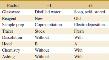
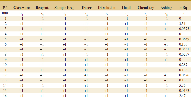
(a) Write down the alias relationships.
(b) Estimate the main effects.
(c) Prepare a normal probability plot for the effects and interpret the results.
![]() 14-60. An article in the Journal of Marketing Research (1973, Vol. 10(3), pp. 270–276) presented a 27−4 fractional factorial design to conduct marketing research:
14-60. An article in the Journal of Marketing Research (1973, Vol. 10(3), pp. 270–276) presented a 27−4 fractional factorial design to conduct marketing research:
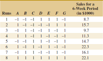
The factors and levels are shown in the following table.
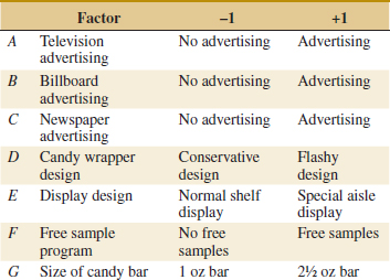
(a) Write down the alias relationships.
(b) Estimate the main effects.
(c) Prepare a normal probability plot for the effects and interpret the results.
![]() 14-61. An article in Bioresource Technology [“Medium Optimization for Phenazine-1-carboxylic Acid Production by a gacA qscR Double Mutant of Pseudomonas sp. M18 Using Response Surface Methodology” (Vol. 101(11), 2010, pp. 4089–4095)] described an experiment to optimize culture medium factors to enhance phenazine-1-carboxylic acid (PCA) production. A 25−1 fractional factorial design was conducted with factors soybean meal, glucose, corn steep liquor, ethanol, and MgSO4. Rows below the horizontal line in the table (coded with zeros) correspond to center points.
14-61. An article in Bioresource Technology [“Medium Optimization for Phenazine-1-carboxylic Acid Production by a gacA qscR Double Mutant of Pseudomonas sp. M18 Using Response Surface Methodology” (Vol. 101(11), 2010, pp. 4089–4095)] described an experiment to optimize culture medium factors to enhance phenazine-1-carboxylic acid (PCA) production. A 25−1 fractional factorial design was conducted with factors soybean meal, glucose, corn steep liquor, ethanol, and MgSO4. Rows below the horizontal line in the table (coded with zeros) correspond to center points.
(a) What is the generator of this design?
(b) What is the resolution of this design?
(c) Analyze factor effects and comment on important ones.
(d) Develop a regression model to predict production in terms of the actual factor levels.
(e) Does a residual analysis indicate any problems?
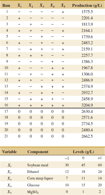
![]()
14-62. An article in Journal of Hazardous Materials [“Statistical Factor-Screening and Optimization in Slurry Phase Bioremediation of 2,4,6-trinitrotoluene Contaminated Soil,” (2011, Vol. 188(1), pp. 1–9)] described an experiment to optimize the removal of TNT 2,4,6-trinitrotoluene (TNT). TNT is a predominant contaminant at ammunition plants, testing facilities and military zones. TNT removal (TR) is measured by the percentage of the initial concentration removed (mg/kg-soil).
A 27−3 fractional factorial design was conducted. The data are in the following table. Rows below the horizontal line in the table (coded with zeros) correspond to center points.
(a) What is the alias structure of this design?
(b) What is the resolution of this design?
(c) Analyze factor effects and comment on important effects.
(d) Develop a regression model to predict removal in terms of the actual factor levels.
(e) Does a residual analysis indicate any problems?
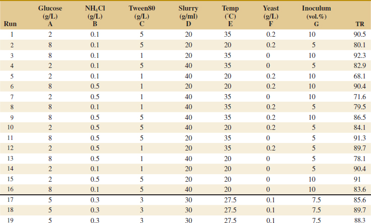
14-8 Response Surface Methods and Designs
Response surface methodology, or RSM, is a collection of mathematical and statistical techniques that are useful for modeling and analysis in applications in which a response of interest is influenced by several variables and the objective is to optimize this response. For example, suppose that a chemical engineer wishes to find the levels of temperature (x1) and feed concentration (x2) that maximize the yield (y) of a process. The process yield is a function of the levels of temperature and feed concentration, say,
![]()
where ![]() represents the noise or error observed in the response Y. If we denote the expected response by E(Y) = f(x1, x2) = η, then the surface represented by
represents the noise or error observed in the response Y. If we denote the expected response by E(Y) = f(x1, x2) = η, then the surface represented by
![]()
is called a response surface.
We may represent the response surface graphically as shown in Fig. 14-42, where η is plotted versus the levels of x1 and x2. Notice that the response is represented as a surface plot in a three-dimensional space. To help visualize the shape of a response surface, we often plot the contours of the response surface as shown in Fig. 14-43. In the contour plot, lines of constant response are drawn in the x1, x2 plane. Each contour corresponds to a particular height of the response surface. The contour plot is helpful in studying the levels of x1 and x2 that result in changes in the shape or height of the response surface.
In most RSM problems, the form of the relationship between the response and the independent variables is unknown. Thus, the first step in RSM is to find a suitable approximation for the true relationship between Y and the independent variables. Usually, a low-order polynomial in some region of the independent variables is employed. If the response is well modeled by a linear function of the independent variables, the approximating function is the first-order model
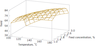
FIGURE 14-42 A three-dimensional response surface showing the expected yield as a function of temperature and feed concentration.
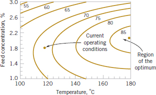
FIGURE 14-43 A contour plot of the yield response surface in Figure 14-42.
![]()
If there is curvature in the system, then a polynomial of higher degree must be used, such as the second-order model
![]()
Many RSM problems use one or both of these approximating polynomials. Of course, it is unlikely that a polynomial model will be a reasonable approximation of the true functional relationship over the entire space of the independent variables, but for a relatively small region, they usually work quite well.
The method of least squares, discussed in Chapters 11 and 12, is used to estimate the parameters in the approximating polynomials. The response surface analysis is then based on the fitted surface. If the fitted surface is an adequate approximation of the true response function, analysis of the fitted surface will be approximately equivalent to analysis of the actual system.
RSM is a sequential procedure. Often, when we are at a point on the response surface that is remote from the optimum, such as the current operating conditions in Fig. 14-43, there is little curvature in the system and the first-order model is appropriate. Our objective here is to lead the experimenter rapidly and efficiently to the general vicinity of the optimum. Once the region of the optimum has been found, a more elaborate model such as the second-order model may be employed, and an analysis may be performed to locate the optimum. From Fig. 14-43, we see that the analysis of a response surface can be thought of as “climbing a hill,” where the top of the hill represents the point of maximum response. If the true optimum is a point of minimum response, we may think of “descending into a valley.”
The eventual objective of RSM is to determine the optimum operating conditions for the system or to determine a region of the factor space in which operating specifications are satisfied. Also note that the word optimum in RSM is used in a special sense. The “hill-climbing” procedures of RSM guarantee convergence to a local optimum only.
Method of Steepest Ascent
Frequently, the initial estimate of the optimum operating conditions for the system is far from the actual optimum. In such circumstances, the objective of the experimenter is to move rapidly to the general vicinity of the optimum. We wish to use a simple and economically efficient experimental procedure. When we are remote from the optimum, we usually assume that a first-order model is an adequate approximation to the true surface in a small region of the x's.
The method of steepest ascent is a procedure for moving sequentially along the path of steepest ascent, that is, in the direction of the maximum increase in the response. Of course, if minimization is desired, we are talking about the method of steepest descent. The fitted first-order model is
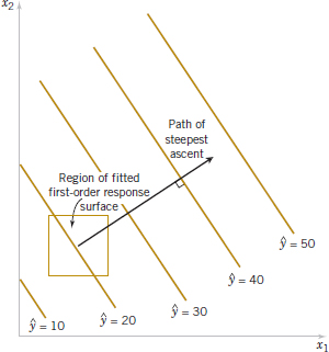
FIGURE 14-44 First-order response surface and path of steepest ascent.
![]()
and the first-order response surface, that is, the contours of ![]() , is a series of parallel lines such as that shown in Fig. 14-44. The direction of steepest ascent is the direction in which
, is a series of parallel lines such as that shown in Fig. 14-44. The direction of steepest ascent is the direction in which ![]() increases most rapidly. This direction is normal to the fitted response surface contours. We usually take as the path of steepest ascent the line through the center of the region of interest and normal to the fitted surface contours. Thus, the steps along the path are proportional to the regression coefficients {
increases most rapidly. This direction is normal to the fitted response surface contours. We usually take as the path of steepest ascent the line through the center of the region of interest and normal to the fitted surface contours. Thus, the steps along the path are proportional to the regression coefficients {![]() i}. The experimenter determines the actual step size based on process knowledge or other practical considerations.
i}. The experimenter determines the actual step size based on process knowledge or other practical considerations.
Experiments are conducted along the path of steepest ascent until no further increase in response is observed. Then a new first-order model may be fit, a new direction of steepest ascent determined, and further experiments conducted in that direction until the experimenter believes that the process is near the optimum.
Example 14-11 Process Yield Steepest Ascent In Example 14-6, we described an experiment on a chemical process in which two factors, reaction time (x1) and reaction temperature (x2), affect the percent conversion or yield (Y). Figure 14-27 shows the 22 design plus five center points used in this study. The engineer found that both factors were important, there was no interaction, and there was no curvature in the response surface. Therefore, the first-order model
![]()
should be appropriate. Now the effect estimate of time is 1.55 hours and the effect estimate of temperature is 0.65°F, and because the regression coefficients ![]() 1 and
1 and ![]() 2 are one-half of the corresponding effect estimates, the fitted first-order model is
2 are one-half of the corresponding effect estimates, the fitted first-order model is
![]()
Figure 14-45(a) and (b) show the contour plot and three-dimensional surface plot of this model. Figure 14-45 also shows the relationship between the coded variables x1 and x2 (that defined the high and low levels of the factors) and the original variables, time (in minutes), and temperature (in °F).
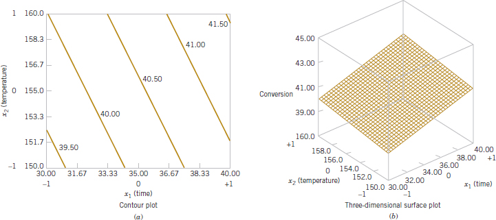
FIGURE 14-45 Response surface plots for the first-order model in Example 14-11.
From examining these plots (or the fitted model), we see that to move away from the design center—the point (x1 = 0, x2 = 0)—along the path of steepest ascent, we would move 0.775 unit in the x1 direction for every 0.325 unit in the x2 direction. Thus, the path of steepest ascent passes through the point (x1 = 0, x2 = 0) and has a slope 0.325/0.775. The engineer decides to use 5 minutes of reaction time as the basic step size. Now, 5 minutes of reaction time is equivalent to a step in the coded variable x1 of Δx1 = 1. Therefore, the steps along the path of steepest ascent are Δx1 = 1.0000 and Δx2 = (0.325/0.775)Δx1 = 0.42. A change of Δx2 = 0.42 in the coded variable x2 is equivalent to about 2°F in the original variable temperature. Therefore, the engineer moves along the path of steepest ascent by increasing reaction time by 5 minutes and temperature by 2°F. An actual observation on yield is determined at each point.
Next Steps: Figure 14-46 shows several points along this path of steepest ascent and the yields actually observed from the process at those points. At points A−D, the observed yield increases steadily, but beyond point D, the yield decreases. Therefore, steepest ascent terminates in the vicinity of 55 minutes of reaction time and 163°F with an observed percent conversion of 67%.
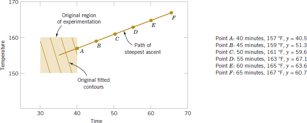
FIGURE 14-46 Steepest ascent experiment for Example 14-11.
Analysis of a Second-Order Response Surface
When the experimenter is relatively close to the optimum, a second-order model is usually required to approximate the response because of curvature in the true response surface. The fitted second-order model is
![]()
where ![]() denotes the least squares estimate of b. In this section, we show how to use this fitted model to find the optimum set of operating conditions for the x's and to characterize the nature of the response surface.
denotes the least squares estimate of b. In this section, we show how to use this fitted model to find the optimum set of operating conditions for the x's and to characterize the nature of the response surface.
Example 14-12 Process Yield Central Composite Design
Continuation of Example 14-11
Consider the chemical process from Example 14-11, where the method of steepest ascent terminated at a reaction time of 55 minutes and a temperature of 163°F. The experimenter decides to fit a second-order model in this region. Table 14-34 and Fig. 14-47 show the experimental design, which consists of a 22 design centered at 55 minutes and 165°F, five center points, and four runs along the coordinate axes called axial runs. This type of design, called a central composite design, is a very popular design for fitting second-order response surfaces.
Two response variables were measured during this phase of the experiment: percentage conversion (yield) and viscosity. The least-squares quadratic model for the yield response is
![]()
The analysis of variance for this model is shown in Table 14-35.
Figure 14-48 shows the response surface contour plot and the three-dimensional surface plot for this model. From examination of these plots, the maximum yield is about 70%, obtained at approximately 60 minutes of reaction time and 167°F.
The viscosity response is adequately described by the first-order model
![]()
Table 14-36 summarizes the analysis of variance for this model. The response surface is shown graphically in Fig. 14-49. Notice that viscosity increases as both time and temperature increase.
![]() TABLE • 14-34 Central Composite Design for Example 14-12
TABLE • 14-34 Central Composite Design for Example 14-12
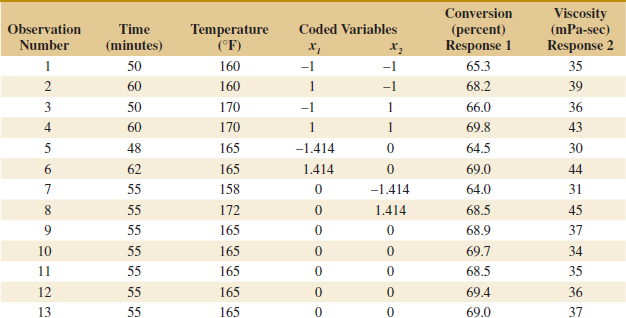
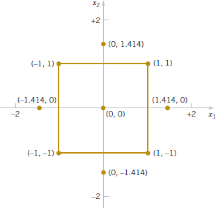
FIGURE 14-47 Central composite design for Example 14-12.
![]() TABLE • 14-35 Analysis of Variance for the Quadratic Model, Yield Response
TABLE • 14-35 Analysis of Variance for the Quadratic Model, Yield Response
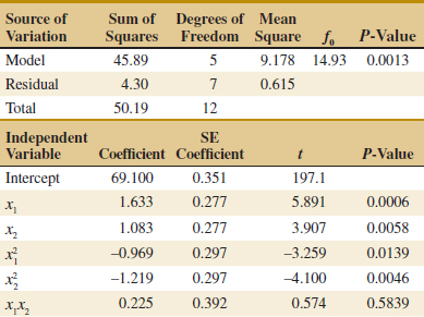
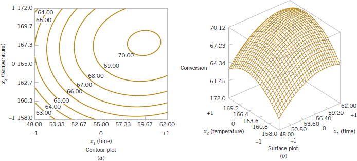
FIGURE 14-48 Response surface plots for the yield response, Example 14-12.
![]() TABLE • 14-36 Analysis of Variance for the First-Order Model, Viscosity Response
TABLE • 14-36 Analysis of Variance for the First-Order Model, Viscosity Response
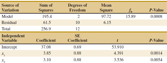
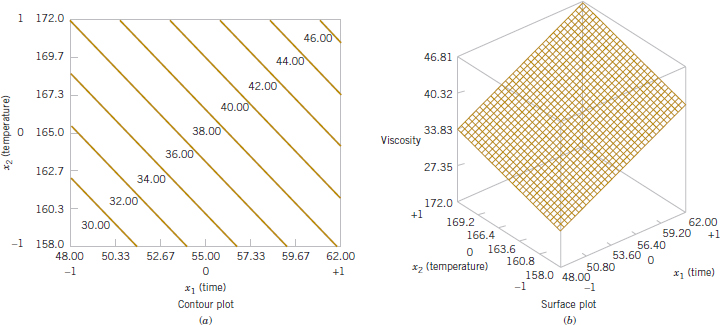
FIGURE 14-49 Response surface plots for the viscosity response, Example 14-12.
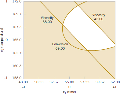
FIGURE 14-50 Overlay of yield and viscosity response surfaces, Example 14-12.
Practical Interpretation: As in most response surface problems, the experimenter in this example had conflicting objectives regarding the two responses. The objective was to maximize yield, but the acceptable range for viscosity was 38 ≤ y2 ≤ 42. When there are only a few independent variables, an easy way to solve this problem is to overlay the response surfaces to find the optimum. Figure 14-50 shows the overlay plot of both responses with the contours y1 = 69% conversion, y2 = 38, and y2 = 42 highlighted. The shaded areas on this plot identify unfeasible combinations of time and temperature. This graph shows that several combinations of time and temperature are satisfactory.
Example 14-12 illustrates the use of a central composite design (CCD) for fitting a second-order response surface model. These designs are widely used in practice because they are relatively efficient with respect to the number of runs required. In general, a CCD in k factors requires 2k factorial runs, 2k axial runs, and at least one center point (three to five center points are typically used). Designs for k = 2 and k = 3 factors are shown in Fig. 14-51.

FIGURE 14-51 Central composite designs for k = 2 and k = 3.
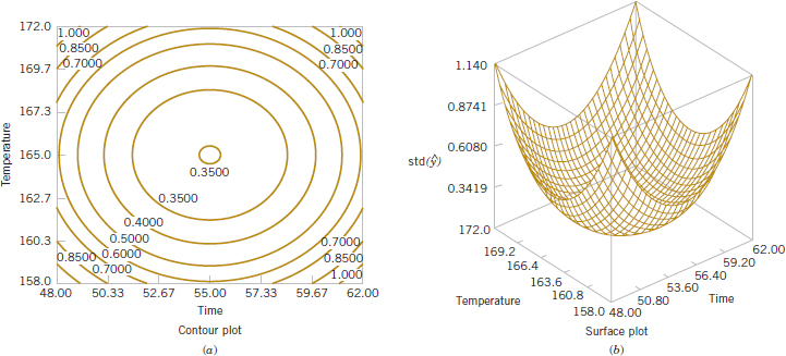
FIGURE 14-52 Plots of constant ![]() for a rotatable central composite design.
for a rotatable central composite design.
The central composite design may be made rotatable by proper choice of the axial spacing α in Fig. 14-51. If the design is rotatable, the standard deviation of predicted response ![]() is constant at all points that are the same distance from the center of the design. For rotatability, choose a = (F)1/4 where F is the number of points in the factorial part of the design (usually F = 2k). For the case of k = 2 factors, α = (22)1/4 = 1.414, as was used in the design in Example 14-12. Figure 14-52 presents a contour plot and a surface plot of the standard deviation of prediction for the quadratic model used for the yield response. Notice that the contours are concentric circles, implying that yield is predicted with equal precision for all points that are the same distance from the center of the design. Also, as one would expect, the precision decreases with increasing distance from the design center.
is constant at all points that are the same distance from the center of the design. For rotatability, choose a = (F)1/4 where F is the number of points in the factorial part of the design (usually F = 2k). For the case of k = 2 factors, α = (22)1/4 = 1.414, as was used in the design in Example 14-12. Figure 14-52 presents a contour plot and a surface plot of the standard deviation of prediction for the quadratic model used for the yield response. Notice that the contours are concentric circles, implying that yield is predicted with equal precision for all points that are the same distance from the center of the design. Also, as one would expect, the precision decreases with increasing distance from the design center.
![]() Problem available in WileyPLUS at instructor's discretion.
Problem available in WileyPLUS at instructor's discretion.
![]() Go Tutorial Tutoring problem available in WileyPLUS at instructor's discretion
Go Tutorial Tutoring problem available in WileyPLUS at instructor's discretion
![]() 14-63.
14-63. ![]() An article in Rubber Age (1961, Vol. 89, pp. 453–458) describes an experiment on the manufacture of a product in which two factors were varied. The factors are reaction time (hr) and temperature (°C). These factors are coded as x1 = (time − 12)/8 and x2 = (temperature − 250)/30. The following data were observed where y is the yield (in percent):
An article in Rubber Age (1961, Vol. 89, pp. 453–458) describes an experiment on the manufacture of a product in which two factors were varied. The factors are reaction time (hr) and temperature (°C). These factors are coded as x1 = (time − 12)/8 and x2 = (temperature − 250)/30. The following data were observed where y is the yield (in percent):
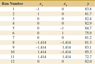
(a) Plot the points at which the experimental runs were made.
(b) Fit a second-order model to the data. Is the second-order model adequate?
(c) Plot the yield response surface. What recommendations would you make about the operating conditions for this process?
![]() 14-64.
14-64. ![]() An article in Quality Engineering [“Mean and Variance Modeling with Qualitative Responses: A Case Study” (1998–1999, Vol. 11, pp. 141–148)] studied how three active ingredients of a particular food affect the overall taste of the product. The measure of the overall taste is the overall mean liking score (MLS). The three ingredients are identified by the variables x1, x2, and x3. The data are shown in the following table.
An article in Quality Engineering [“Mean and Variance Modeling with Qualitative Responses: A Case Study” (1998–1999, Vol. 11, pp. 141–148)] studied how three active ingredients of a particular food affect the overall taste of the product. The measure of the overall taste is the overall mean liking score (MLS). The three ingredients are identified by the variables x1, x2, and x3. The data are shown in the following table.
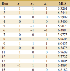
(a) Fit a second-order response surface model to the data.
(b) Construct contour plots and response surface plots for MLS. What are your conclusions?
(c) Analyze the residuals from this experiment. Does your analysis indicate any potential problems?
(d) This design has only a single center point. Is this a good design in your opinion?
14-65. ![]() Consider the first-order model
Consider the first-order model
![]()
where −1 ≤ xi ≤ 1. Find the direction of steepest ascent.
14-66. ![]() A manufacturer of cutting tools has developed two empirical equations for tool life (y1) and tool cost (y2). Both models are functions of tool hardness (x1) and manufacturing time (x2). The equations are
A manufacturer of cutting tools has developed two empirical equations for tool life (y1) and tool cost (y2). Both models are functions of tool hardness (x1) and manufacturing time (x2). The equations are
![]()
and both are valid over the range −1.5 ≤ xi ≤ 1.5. Suppose that tool life must exceed 12 hours and cost must be below $27.50.
(a) Is there a feasible set of operating conditions?
(b) Where would you run this process?
![]()
14-67. ![]() An article in Tappi (1960, Vol. 43, pp. 38–44) describes an experiment that investigated the ash value of paper pulp (a measure of inorganic impurities). Two variables, temperature T in degrees Celsius and time t in hours, were studied, and some of the results are shown in the following table. The coded predictor variables shown are
An article in Tappi (1960, Vol. 43, pp. 38–44) describes an experiment that investigated the ash value of paper pulp (a measure of inorganic impurities). Two variables, temperature T in degrees Celsius and time t in hours, were studied, and some of the results are shown in the following table. The coded predictor variables shown are
![]()
and the response y is (dry ash value in %) × 103.
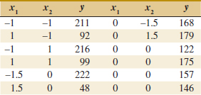
(a) What type of design has been used in this study? Is the design rotatable?
(b) Fit a quadratic model to the data. Is this model satisfactory?
(c) If it is important to minimize the ash value, where would you run the process?
![]()
14-68. ![]() In their book Empirical Model Building and Response Surfaces (John Wiley, 1987), Box and Draper described an experiment with three factors. The data in the following table are a variation of the original experiment from their book. Suppose that these data were collected in a semiconductor manufacturing process.
In their book Empirical Model Building and Response Surfaces (John Wiley, 1987), Box and Draper described an experiment with three factors. The data in the following table are a variation of the original experiment from their book. Suppose that these data were collected in a semiconductor manufacturing process.
(a) The response y1 is the average of three readings on resistivity for a single wafer. Fit a quadratic model to this response.
(b) The response y2 is the standard deviation of the three resistivity measurements. Fit a linear model to this response.
(c) Where would you recommend that we set x1, x2, and x3 if the objective is to hold mean resistivity at 500 and minimize the standard deviation?
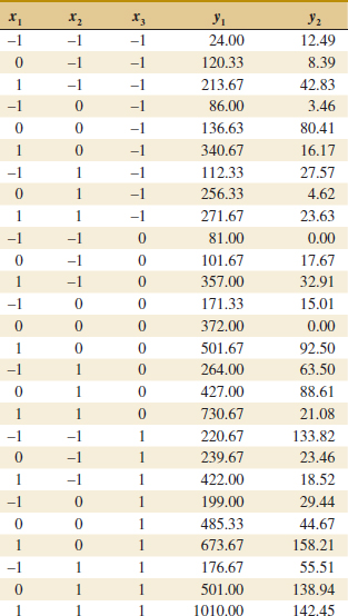
14-69. Consider the first-order model
![]()
where −1 ≤ xi ≤ 1.
(a) Find the direction of steepest ascent.
(b) Assume that the current design is centered at the point (0, 0, 0, 0). Determine the point that is three units from the current center point in the direction of steepest ascent.
14-70. Suppose that a response y1 is a function of two inputs x1 and x2 with y1 = ![]() .
.
(a) Draw the contours of this response function.
(b) Consider another response y2 = (x1 − 2)2 + (x2 − 3)2.
(c) Add the contours for y2 and discuss how feasible it is to minimize both y1 and y2 with values for x1 and x2.
14-71. Two responses y1 and y2 are related to two inputs x1 and x2 by the models y1 = 5 + (x1 − 2)2 + (x2 − 3)2 and y2 = x2 − x1 + 3.
Suppose that the objectives are y1 ≤ 9 and y2 ≥ 6.
(a) Is there a feasible set of operating conditions for x1 and x2? If so, plot the feasible region in the space of x1 and x2.
(b) Determine the point(s) (x1, x2) that yields y2 ≥ 6 and minimizes y1.
14-72. An article in the Journal of Materials Processing Technology (1997, Vol. 67, pp. 55–61) used response surface methodology to generate surface roughness prediction models for turning EN 24T steel (290 BHN). The data are shown in the following table.
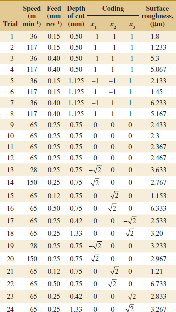
The factors and levels for the experiment are shown in Table E14-3.
(a) Plot the points at which the experimental runs were made.
(b) Fit both first-and second-order models to the data. Comment on the adequacies of these models.
(c) Plot the roughness response surface for the second-order model and comment.
![]() 14-73. An article in Analytical Biochemistry [“Application of Central Composite Design for DNA Hybridization Onto Magnetic Microparticles,” (2009, Vol. 391(1), 2009, pp. 17–23)] considered the effects of probe and target concentration and particle number in immobilization and hybridization on a micro particle-based DNA hybridization assay. Mean fluorescence is the response. Particle concentration was transformed to surface area measurements. Other concentrations were measured in micromoles per liter (μM). Data are in Table E14-2.
14-73. An article in Analytical Biochemistry [“Application of Central Composite Design for DNA Hybridization Onto Magnetic Microparticles,” (2009, Vol. 391(1), 2009, pp. 17–23)] considered the effects of probe and target concentration and particle number in immobilization and hybridization on a micro particle-based DNA hybridization assay. Mean fluorescence is the response. Particle concentration was transformed to surface area measurements. Other concentrations were measured in micromoles per liter (μM). Data are in Table E14-2.
(a) What type of design is used?
(b) Fit a second-order response surface model to the data.
(c) Does a residual analysis indicate any problems?
![]() 14-74. An article in Applied Biochemistry and Biotechnology (“A Statistical Approach for Optimization of Polyhydroxybutyrate Production by Bacillus sphaericus NCIM 5149 under Submerged Fermentation Using Central Composite Design” (2010, Vol. 162(4), pp. 996–1007)] described an experiment to optimize the production of polyhydroxybutyrate (PHB). Inoculum age, pH, and substrate were selected as factors, and a central composite design was conducted. Data follow.
14-74. An article in Applied Biochemistry and Biotechnology (“A Statistical Approach for Optimization of Polyhydroxybutyrate Production by Bacillus sphaericus NCIM 5149 under Submerged Fermentation Using Central Composite Design” (2010, Vol. 162(4), pp. 996–1007)] described an experiment to optimize the production of polyhydroxybutyrate (PHB). Inoculum age, pH, and substrate were selected as factors, and a central composite design was conducted. Data follow.
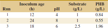
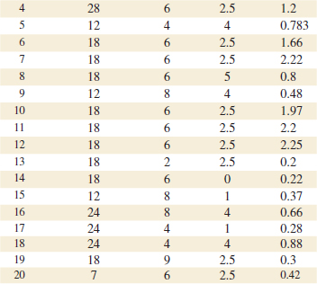
(a) Plot the points at which the experimental runs were made [Hint: Code each variable first.] What type of design is used?
(b) Fit a second-order response surface model to the data.
(c) Does a residual analysis indicate any problems?
(d) Construct a contour plot and response surface for PHB amount in terms of two factors.
(e) Can you recommend values for inoculum age, pH and substrate to maximize production?
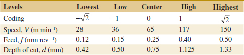
Supplemental Exercises
![]() Problem available in WileyPLUS at instructor's discretion.
Problem available in WileyPLUS at instructor's discretion.
![]() Go Tutorial Tutoring problem available in WileyPLUS at instructor's discretion.
Go Tutorial Tutoring problem available in WileyPLUS at instructor's discretion.
![]() 14-75.
14-75. ![]() An article in Process Engineering (1992, No. 71, pp. 46–47) presented a two-factor factorial experiment to investigate the effect of pH and catalyst concentration on product viscosity (cSt). The data are as follows:
An article in Process Engineering (1992, No. 71, pp. 46–47) presented a two-factor factorial experiment to investigate the effect of pH and catalyst concentration on product viscosity (cSt). The data are as follows:
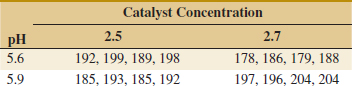
(a) Test for main effects and interactions using α = 0.05. What are your conclusions?
(b) Graph the interaction and discuss the information provided by this plot.
(c) Analyze the residuals from this experiment.
14-76. ![]() Heat-treating metal parts is a widely used manufacturing process. An article in the Journal of Metals (1989, Vol. 41) described an experiment to investigate flatness distortion from heat-treating for three types of gears and two heat-treating times. The data follow:
Heat-treating metal parts is a widely used manufacturing process. An article in the Journal of Metals (1989, Vol. 41) described an experiment to investigate flatness distortion from heat-treating for three types of gears and two heat-treating times. The data follow:
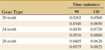
![]() TABLE • E14-2 Fluorescence Experiment
TABLE • E14-2 Fluorescence Experiment
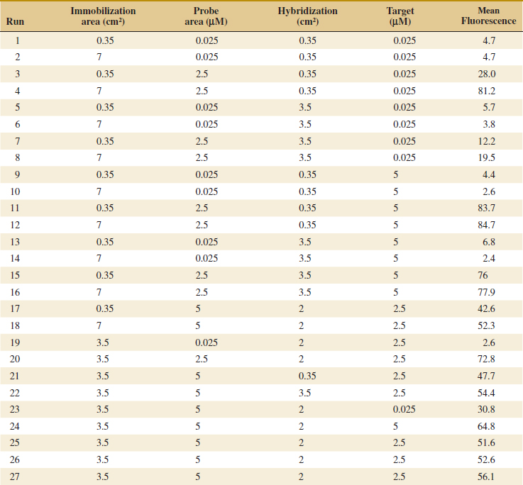
(a) Is there any evidence that flatness distortion is different for the different gear types? Is there any indication that heat-treating time affects the flatness distortion? Do these factors interact? Use α = 0.05.
(b) Construct graphs of the factor effects that aid in drawing conclusions from this experiment.
(c) Analyze the residuals from this experiment. Comment on the validity of the underlying assumptions.
14-77. An article in the Textile Research Institute Journal (1984, Vol. 54, pp. 171–179) reported the results of an experiment that studied the effects of treating fabric with selected inorganic salts on the flammability of the material. Two application levels of each salt were used, and a vertical burn test was used on each sample. (This finds the temperature at which each sample ignites.) The burn test data follow.
![]()
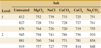
(a) Test for differences between salts, application levels, and interactions. Use α = 0.01.
(b) Draw a graph of the interaction between salt and application level. What conclusions can you draw from this graph?
(c) Analyze the residuals from this experiment.
14-78. ![]() An article in the IEEE Transactions on Components, Hybrids, and Manufacturing Technology (1992, Vol. 15) described an experiment for aligning optical chips onto circuit boards. The method involves placing solder bumps onto the bottom of the chip. The experiment used three solder bump sizes and three alignment methods. The response variable is alignment accuracy (in micrometers). The data are as follows:
An article in the IEEE Transactions on Components, Hybrids, and Manufacturing Technology (1992, Vol. 15) described an experiment for aligning optical chips onto circuit boards. The method involves placing solder bumps onto the bottom of the chip. The experiment used three solder bump sizes and three alignment methods. The response variable is alignment accuracy (in micrometers). The data are as follows:
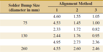
(a) Is there any indication that either solder bump size or alignment method affects the alignment accuracy? Is there any evidence of interaction between these factors? Use a = 0.05.
(b) What recommendations would you make about this process?
(c) Analyze the residuals from this experiment. Comment on model adequacy.
![]() 14-79.
14-79. ![]() An article in Solid State Technology (1984, Vol. 29, pp. 281–284) described the use of factorial experiments in photolithography, an important step in the process of manufacturing integrated circuits. The variables in this experiment (all at two levels) are prebake temperature (A), prebake time (B), and exposure energy (C), and the response variable is delta line width, the difference between the line on the mask and the printed line on the device. The data are as follows: (1) = −2.30, a = −9.87, b = −18.20, ab = −30.20, c = −23.80, ac = −4.30, bc = −3.80, and abc = −14.70.
An article in Solid State Technology (1984, Vol. 29, pp. 281–284) described the use of factorial experiments in photolithography, an important step in the process of manufacturing integrated circuits. The variables in this experiment (all at two levels) are prebake temperature (A), prebake time (B), and exposure energy (C), and the response variable is delta line width, the difference between the line on the mask and the printed line on the device. The data are as follows: (1) = −2.30, a = −9.87, b = −18.20, ab = −30.20, c = −23.80, ac = −4.30, bc = −3.80, and abc = −14.70.
(a) Estimate the factor effects.
(b) Use a normal probability plot of the effect estimates to identity factors that may be important.
(c) What model would you recommend for predicting the delta line width response based on the results of this experiment?
(d) Analyze the residuals from this experiment, and comment on model adequacy.
![]() 14-80.
14-80. ![]() An article in the Journal of Coatings Technology (1988, Vol. 60, pp. 27–32) described a 24 factorial design used for studying a silver automobile basecoat. The response variable is distinctness of image (DOI). The variables used in the experiment are
An article in the Journal of Coatings Technology (1988, Vol. 60, pp. 27–32) described a 24 factorial design used for studying a silver automobile basecoat. The response variable is distinctness of image (DOI). The variables used in the experiment are
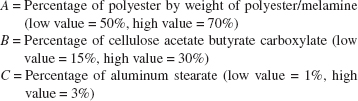
![]()
The responses are (1) = 63.8, a = 77.6, b = 68.8, ab = 76.5, c = 72.5, ac = 77.2, bc = 77.7, abc = 84.5, d = 60.6, ad = 64.9, bd = 72.7, abd = 73.3, cd = 68.0, acd = 76.3, bcd = 76.0, and abcd = 75.9.
(a) Estimate the factor effects.
(b) From a normal probability plot of the effects, identify a tentative model for the data from this experiment.
(c) Using the apparently negligible factors as an estimate of error, test for significance of the factors identified in part (b). Use a = 0.05.
![]()
(d) What model would you use to describe the process based on this experiment? Interpret the model.
(e) Analyze the residuals from the model in part (d) and comment on your findings.
![]()
14-81. An article in the Journal of Manufacturing Systems (1991, vol. 10, pp. 32–40) described an experiment to investigate the effect of four factors, P = waterjet pressure, F = abrasive flow rate, G = abrasive grain size, and V = jet traverse speed, on the surface roughness of a waterjet cutter. A 24 design follows.
(a) Estimate the factor effects.
(b) Form a tentative model by examining a normal probability plot of the effects.
(c) Is the model in part (b) a reasonable description of the process? Is lack of fit significant? Use a = 0.05.
(d) Interpret the results of this experiment.
(e) Analyze the residuals from this experiment.
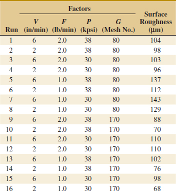
![]()
14-82. Construct a ![]() design for the problem in Exercise 14-80. Select the data for the eight runs that would have been required for this design. Analyze these runs and compare your conclusions to those obtained in Exercise 14-80 for the full factorial.
design for the problem in Exercise 14-80. Select the data for the eight runs that would have been required for this design. Analyze these runs and compare your conclusions to those obtained in Exercise 14-80 for the full factorial.
![]()
14-83. Construct a ![]() design for the problem in Exercise 14-81. Select the data for the eight runs that would have been required for this design. Analyze these data and compare your conclusions to those obtained in Exercise 14-81 for the full factorial.
design for the problem in Exercise 14-81. Select the data for the eight runs that would have been required for this design. Analyze these data and compare your conclusions to those obtained in Exercise 14-81 for the full factorial.
14-84. Construct a ![]() design in 16 runs. What are the alias relationships in this design?
design in 16 runs. What are the alias relationships in this design?
14-85. Construct a ![]() design in eight runs. What are the alias relationships in this design?
design in eight runs. What are the alias relationships in this design?
![]() 14-86. An article in the Journal of Quality Technology (1985, Vol. 17, pp. 198–206) described the use of a replicated fractional factorial to investigate the effect of five factors on the free height of leaf springs used in an automotive application. The factors are A = furnace temperature, B = heating time, C = transfer time, D = hold down time, and E = quench oil temperature. The data are shown in the following table.
14-86. An article in the Journal of Quality Technology (1985, Vol. 17, pp. 198–206) described the use of a replicated fractional factorial to investigate the effect of five factors on the free height of leaf springs used in an automotive application. The factors are A = furnace temperature, B = heating time, C = transfer time, D = hold down time, and E = quench oil temperature. The data are shown in the following table.
(a) What is the generator for this fraction? Write out the alias structure.
(b) Analyze the data. What factors influence mean free height?
(c) Calculate the range of free height for each run. Is there any indication that any of these factors affect variability in free height?
(d) Analyze the residuals from this experiment and comment on your findings.
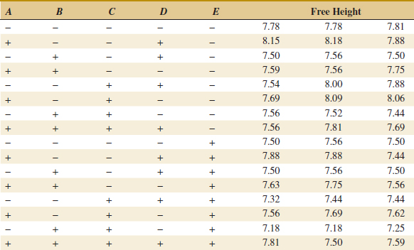
![]() 14-87. An article in Rubber Chemistry and Technology (Vol. 47, 1974, pp. 825–836) described an experiment to study the effect of several variables on the Mooney viscosity of rubber, including silica filler (parts per hundred) and oil filler (parts per hundred). Data typical of that reported in this experiment are reported in the following table where
14-87. An article in Rubber Chemistry and Technology (Vol. 47, 1974, pp. 825–836) described an experiment to study the effect of several variables on the Mooney viscosity of rubber, including silica filler (parts per hundred) and oil filler (parts per hundred). Data typical of that reported in this experiment are reported in the following table where
![]()
(a) What type of experimental design has been used?
(b) Analyze the data and draw appropriate conclusions.
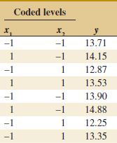
![]() 14-88.
14-88. ![]() An article in Tropical Science [“Proximate Composition of the Seeds of Acacia Nilotica var Adansonti (Bagaruwa) and Extraction of Its Protein” (1992, Vol. 32(3), pp. 263–268)] reported on research extracting and concentrating the proteins of the bagaruwa seeds in livestock feeding in Nigeria to eliminate the toxic substances from the seeds. The following are the effects of extraction time and flour to solvent ratio on protein extractability of the bagaruwa seeds in distilled water:
An article in Tropical Science [“Proximate Composition of the Seeds of Acacia Nilotica var Adansonti (Bagaruwa) and Extraction of Its Protein” (1992, Vol. 32(3), pp. 263–268)] reported on research extracting and concentrating the proteins of the bagaruwa seeds in livestock feeding in Nigeria to eliminate the toxic substances from the seeds. The following are the effects of extraction time and flour to solvent ratio on protein extractability of the bagaruwa seeds in distilled water:
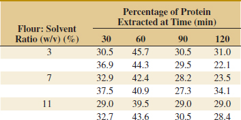
All values are means of three determinations.
(a) Test the appropriate hypotheses and draw conclusions using the analysis of variance with α = 0.5.
(b) Graphically analyze the interaction.
(c) Analyze the residuals from this experiment.
![]()
14-89. ![]() An article in Plant Disease [“Effect of Nitrogen and Potassium Fertilizer Rates on Severity of Xanthomonas Blight of Syngonium Podophyllum” (1989, Vol. 73(12), pp. 972–975)] showed the effect of the variable nitrogen and potassium rates on the growth of “White Butterfly” and the mean percentage of disease. Data representative of that collected in this experiment is provided in the following table.
An article in Plant Disease [“Effect of Nitrogen and Potassium Fertilizer Rates on Severity of Xanthomonas Blight of Syngonium Podophyllum” (1989, Vol. 73(12), pp. 972–975)] showed the effect of the variable nitrogen and potassium rates on the growth of “White Butterfly” and the mean percentage of disease. Data representative of that collected in this experiment is provided in the following table.
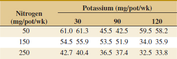
(a) State the appropriate hypotheses.
(b) Use the analysis of variance to test these hypotheses with α = 0.05.
(c) Graphically analyze the residuals from this experiment.
(d) Estimate the appropriate variance components.
![]() 14-90.
14-90. ![]() An article in Biotechnology Progress (2001, Vol. 17, pp. 366–368) reported on an experiment to investigate and optimize the operating conditions of the nisin extraction in aqueous two-phase systems (ATPS). A 22 full factorial design with center points was used to verify the most significant factors affecting the nisin recovery. The factor x1 was the concentration (% w/w) of PEG 4000 and x2 was the concentration (% w/w) of Na2SO4. See the following table for the range and levels of the variables investigated in this study. Nisin extraction is a ratio representing the concentration of nisin, and this was the response y.
An article in Biotechnology Progress (2001, Vol. 17, pp. 366–368) reported on an experiment to investigate and optimize the operating conditions of the nisin extraction in aqueous two-phase systems (ATPS). A 22 full factorial design with center points was used to verify the most significant factors affecting the nisin recovery. The factor x1 was the concentration (% w/w) of PEG 4000 and x2 was the concentration (% w/w) of Na2SO4. See the following table for the range and levels of the variables investigated in this study. Nisin extraction is a ratio representing the concentration of nisin, and this was the response y.
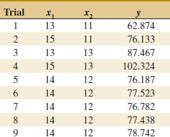
(a) Compute an ANOVA table for the effects and test for curvature with α = 0.05. Is curvature important in this region of the factors?
(b) Calculate residuals from the linear model and test for adequacy of your model.
(c) In a new region of factor space, a central composite design (CCD) was used to perform second-order optimization. The results are shown in the following table. Fit a second-order model to this data and make conclusions.
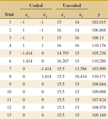
![]()
14-91. An article in the Journal of Applied Electrochemistry (May 2008, Vol. 38(5), pp. 583–590) presented a 27−3 fractional factorial design to perform optimization of polybenzimidazole-based membrane electrode assemblies for H2/O2 fuel cells. The design and data are shown in the following table.
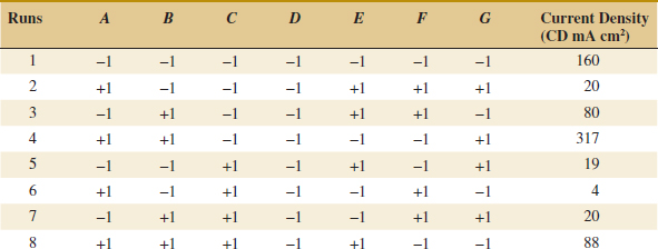
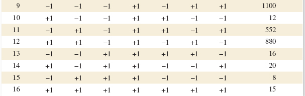
The factors and levels are shown in the following table.
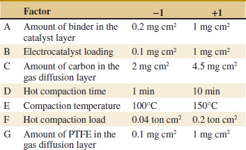
(a) Write down the alias relationships.
(b) Estimate the main effects.
(c) Prepare a normal probability plot for the effects and interpret the results.
(d) Calculate the sum of squares for the alias set that contains the ABG interaction from the corresponding effect estimate.
![]()
14-92. An article in Biotechnology Progress (December 2002, Vol. 18(6), pp. 1170–1175) presented a 27−3 fractional factorial to evaluate factors promoting astaxanthin production. The data are shown in the following table.
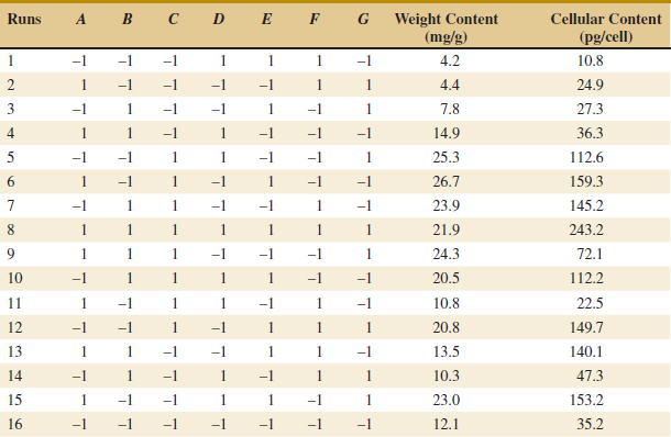
The factors and levels are shown in the following table.
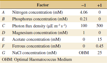
(a) Write down the complete defining relation and the aliases from the design.
(b) Estimate the main effects.
(c) Plot the effect estimates on normal probability paper and interpret the results.
![]() 14-93. The rework time required for a machine was found to depend on the speed at which the machine was run (A), the lubricant used while working (B), and the hardness of the metal used in the machine (C). Two levels of each factor were chosen and a single replicate of a 23 experiment was run. The rework time data (in hours) are shown in the following table.
14-93. The rework time required for a machine was found to depend on the speed at which the machine was run (A), the lubricant used while working (B), and the hardness of the metal used in the machine (C). Two levels of each factor were chosen and a single replicate of a 23 experiment was run. The rework time data (in hours) are shown in the following table.
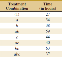
(a) These treatments cannot all be run under the same conditions. Set up a design to run these observations in two blocks of four observations each, with ABC confounded with blocks.
(b) Analyze the data.
14-94. Consider the following results from a two-factor experiment with two levels for factor A and three levels for factor B. Each treatment has three replicates.
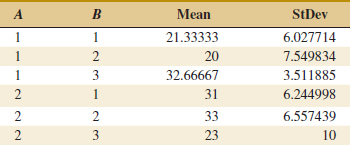
(a) Calculate the sum of squares for each factor and the interaction.
(b) Calculate the sum of squares total and error.
(c) Complete an ANOVA table with F-statistics.
14-95. Consider the following ANOVA table from a two-factor factorial experiment.
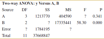
(a) How many levels of each factor were used in the experiment?
(b) How many replicates were used?
(c) What assumption is made in order to obtain an estimate of error?
(d) Calculate the missing entries (denoted with “?”) in the ANOVA table.
![]()
14-96. An article in Process Biochemistry (Dec. 1996, Vol. 31(8), pp. 773–785) presented a 27−3 fractional factorial to perform optimization of manganese dioxide bioleaching media. The data are shown in the following table.
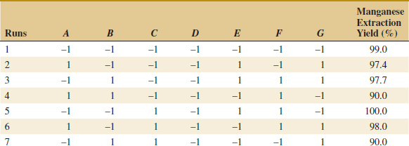
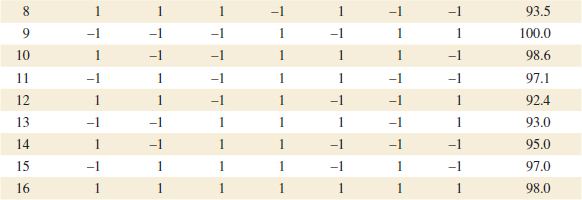
The factors and levels are shown in the following table.
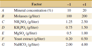
(a) Write down the complete defining relation and the aliases from the design.
(b) Estimate the main effects.
(c) Plot the effect estimates on normal probability paper and interpret the results
(d) Conduct a residual analysis.
![]()
14-97. An article in European Food Research and Technology [“Factorial Design Optimisation of Grape (Vitis vinifera) Seed Polyphenol Extraction” (2009, Vol. 229(5), pp. 731–742)] used a central composite design to study the effects of basic factors (time, ethanol, and pH) on the extractability of polyphenolic phytochemicals from grape seeds. Total ployphenol (TP in mg gallic acid equivalents/100 g dry weight) from three types of grape seeds (Savatiano, Moschofilero, and Agiorgitiko) were recorded. The data follow.
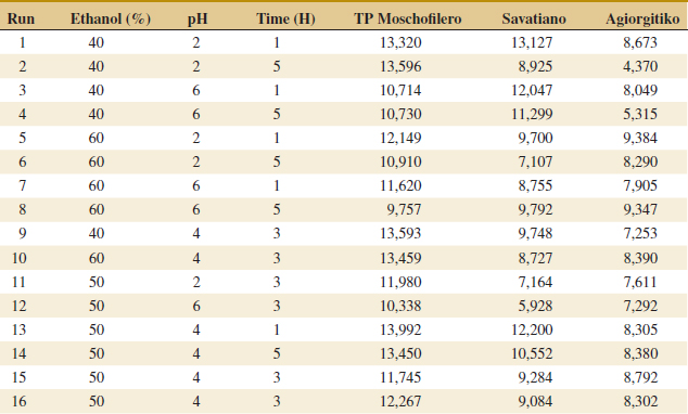
(a) Build a second-order model for each seed type and compare the models.
(b) Comment on the importance of any interaction terms or second-order terms in the models from part (a).
(c) Analyze the residuals from each model.
![]()
14-98. Consider the data in Exercise 14-97. Use only the first eight rows of data from the 23 factorial design and assume that the experiment was conducted in blocks based on seed type.
(a) Analyze the factorial effects and comment on which effects are important.
(b) Develop a regression model to predict the response in terms of the actual factor levels.
(c) Does a residual analysis indicate any problems?
14-99. Graphically study the assumption of no interactions between blocks and treatments in the previous exercise.
![]() 14-100. An article in Journal of Applied Microbiology [“Use of Response Surface Methodology to Optimize Protease Synthesis by a Novel Strain of Bacillus sp. Isolated from Portuguese Sheep Wool” (2012, Vol. 113(1), pp. 36–43)] described a fractional factorial design with three center points to study six factors (yeast extract, peptone, inoculum concentration, agitation, temperature, and pH) for protease activity. Response units were proteolytic activity per ml (U/ml). The data follow.
14-100. An article in Journal of Applied Microbiology [“Use of Response Surface Methodology to Optimize Protease Synthesis by a Novel Strain of Bacillus sp. Isolated from Portuguese Sheep Wool” (2012, Vol. 113(1), pp. 36–43)] described a fractional factorial design with three center points to study six factors (yeast extract, peptone, inoculum concentration, agitation, temperature, and pH) for protease activity. Response units were proteolytic activity per ml (U/ml). The data follow.
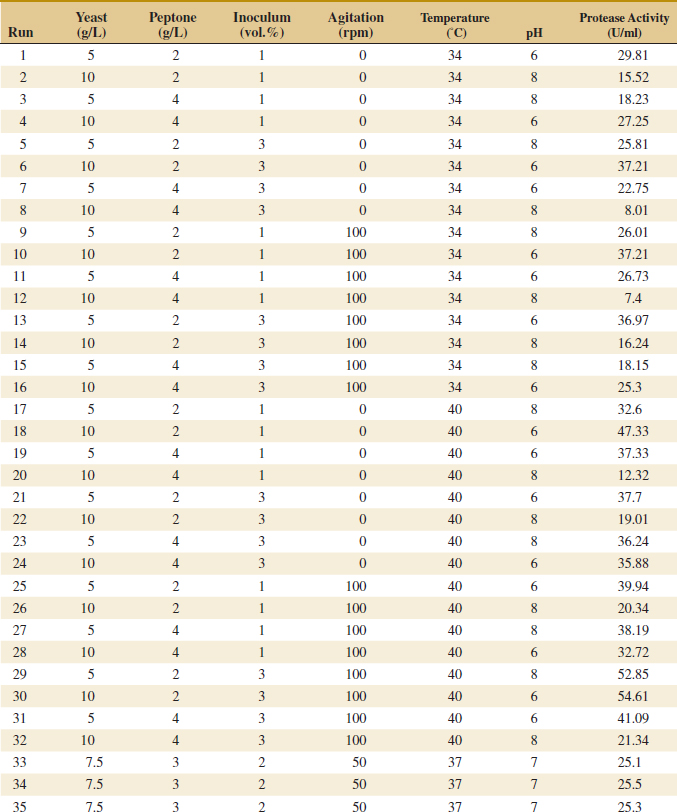
14-101. Consider an unreplicated 2k factorial, and suppose that one of the treatment combinations is missing. One logical approach to this problem is to estimate the missing value with a number that makes the highest order interaction estimate zero. Apply this technique to the data in Example 14-5, assuming that ab is missing. Compare the results of the analysis of the application of these data with the results in Example 14-5.
14-102. What blocking scheme would you recommend if it were necessary to run a 24 design in four blocks of four runs each?
14-103. Consider a 22 design in two blocks with AB confounded with blocks. Prove algebraically that SSAB = SSBlocks.
14-104. Consider a 23 design. Suppose that the largest number of runs that can be made in one block is four, but you can afford to perform a total of 32 observations.
(a) Suggest a blocking scheme will provides some information on all interactions.
(b) Show an outline (source of variability, degrees of freedom only) for the analysis of variance for this design.
14-105. Construct a 25−1 design. Suppose that it is necessary to run this design in two blocks of eight runs each. Show how this can be done by confounding a two-factor interaction (and its aliased three-factor interaction) with blocks.
14-106. Construct a ![]() design. Show how this design may be confounded in four blocks of eight runs each. Are any two-factor interactions confounded with blocks?
design. Show how this design may be confounded in four blocks of eight runs each. Are any two-factor interactions confounded with blocks?
14-107. Construct a ![]() design. Show how this design can be confounded in two blocks of eight runs each without losing information on any of the two-factor interactions.
design. Show how this design can be confounded in two blocks of eight runs each without losing information on any of the two-factor interactions.
14-108. Set up a ![]() design using D = AB, E = AC, F = BC, and G = ABC as the design generators. Ignore all interactions above two factors.
design using D = AB, E = AC, F = BC, and G = ABC as the design generators. Ignore all interactions above two factors.
(a) Verify that each main effect is aliased with three two-factor interactions.
(b) Suppose that a second ![]() design with generators D = −AB, E = −AC, F = −BC, and G = ABC is run. What are the aliases of the main effects in this design?
design with generators D = −AB, E = −AC, F = −BC, and G = ABC is run. What are the aliases of the main effects in this design?
(c) What factors may be estimated if the two sets of factor effect estimates above are combined?
14-109. Consider the square root of the sum of squares for curvature and divide by the square root of mean square error. Explain why the statistic that results has a t distribution and why it can be used to conduct a t test for curvature that is equivalent to the F test in the ANOVA.
Important Terms and Concepts
Aliases
Analysis of variance (ANOVA)
Blocking and nuisance factors
Center points
Central composite design
Confounding
Contrast
Defining relation
Design matrix
Factorial experiment
Fractional factorial design
Generator
Interaction
Main effect
Normal probability plot of factor effects
Optimization experiment
Orthogonal design
Projection property
Regression model
Residual analysis
Resolution
Response surface
Screening experiment
Steepest ascent (or descent)
2k factorial design (Two-level factorial design)