

Statistical Inference for Two Samples

Chapter Outline
10-1 Inference on the Difference in Means of Two Normal Distributions, Variances Known
10-1.1 Hypothesis Tests on the Difference in Means, Variances Known
10-1.2 Type II Error and Choice of Sample Size
10-1.3 Confidence Interval on the Difference in Means, Variances Known
10-2 Inference on the Difference in Means of Two Normal Distributions, Variances Unknown
10-2.1 Hypothesis Tests on the Difference in Means, Variances Unknown
10-2.2 Type II Error and Choice of Sample Size
10-2.3 Confidence Interval on the Difference in Means, Variances Unknown
10-3 A Nonparametric Test on the Difference in Two Means
10-3.1 Description of the Wilcoxon Rank-Sum Test
10-3.2 Large-Sample Approximation
10-3.3 Comparison to the t-Test
10-5 Inference on the Variances of Two Normal Distributions
10-5.2 Hypothesis Tests on the Ratio of Two Variances
10-5.3 Type II Error and Choice of Sample Size
10-5.4 Confidence Interval on the Ratio of Two Variances
10-6 Inference on Two Population Proportions
10-6.1 Large-Sample Tests on the Difference in Population Proportions
10-6.2 Type II Error and Choice of Sample Size
10-6.3 Confidence Interval on the Difference in Population Proportions
10-7 Summary Table and Road Map for Inference Procedures for Two Samples
The safety of drinking water is a serious public health issue. An article in the Arizona Republic on May 27, 2001, reported on arsenic contamination in the water sampled from 10 communities in the metropolitan Phoenix area and 10 communities from rural Arizona. The data showed dramatic differences in the arsenic concentration, ranging from 3 parts per billion (ppb) to 48 ppb. This article suggested some important questions. Does real difference in the arsenic concentrations in the Phoenix area and in the rural communities in Arizona exist? How large is this difference? Is it large enough to require action on the part of the public health service and other state agencies to correct the problem? Are the levels of reported arsenic concentration large enough to constitute a public health risk?
Some of these questions can be answered by statistical methods. If we think of the metropolitan Phoenix communities as one population and the rural Arizona communities as a second population, we could determine whether a statistically significant difference in the mean arsenic concentration exists for the two populations by testing the hypothesis that the two means, say, μ1 and μ2, are different. This is a relatively simple extension to two samples of the one-sample hypothesis testing procedures of Chapter 9. We could also use a confidence interval to estimate the difference in the two means, say, μ1 − μ2.
The arsenic concentration problem is very typical of many problems in engineering and science that involve statistics. Some of the questions can be answered by the application of appropriate statistical tools, and other questions require using engineering or scientific knowledge and expertise to answer satisfactorily.
![]() Learning Objectives
Learning Objectives
After careful study of this chapter, you should be able to do the following:
- Structure comparative experiments involving two samples as hypothesis tests
- Test hypotheses and construct confidence intervals on the difference in means of two normal distributions
- Test hypotheses and construct confidence intervals on the ratio of the variances or standard deviations of two normal distributions
- Test hypotheses and construct confidence intervals on the difference in two population proportions
- Use the P-value approach for making decisions in hypotheses tests
- Compute power, and type II error probability, and make sample size decisions for two-sample tests on means, variances, and proportions
- Explain and use the relationship between confidence intervals and hypothesis tests
10-1 Inference on the Difference in Means of Two Normal Distributions, Variances Known
The previous two chapters presented hypothesis tests and confidence intervals for a single population parameter (the mean μ, the variance σ2, or a proportion p). This chapter extends those results to the case of two independent populations.
The general situation is shown in Fig. 10-1. Population 1 has mean μ1 and variance ![]() , and population 2 has mean μ2 and variance
, and population 2 has mean μ2 and variance ![]() . Inferences will be based on two random samples of sizes n1 and n2, respectively. That is, X11, X12,..., X1n1 is a random sample of n1 observations from population 1, and X21, X22,..., X2n2 is a random sample of n2 observations from population 2. Most of the practical applications of the procedures in this chapter arise in the context of simple comparative experiments in which the objective is to study the difference in the parameters of the two populations.
. Inferences will be based on two random samples of sizes n1 and n2, respectively. That is, X11, X12,..., X1n1 is a random sample of n1 observations from population 1, and X21, X22,..., X2n2 is a random sample of n2 observations from population 2. Most of the practical applications of the procedures in this chapter arise in the context of simple comparative experiments in which the objective is to study the difference in the parameters of the two populations.
Engineers and scientists are often interested in comparing two different conditions to determine whether either condition produces a significant effect on the response that is observed. These conditions are sometimes called treatments. Example 10-1 described such an experiment; the two different treatments are two paint formulations, and the response is the drying time. The purpose of the study is to determine whether the new formulation results in a significant effect—reducing drying time. In this situation, the product developer (the experimenter) randomly assigned 10 test specimens to one formulation and 10 test specimens to the other formulation. Then the paints were applied to the test specimens in random order until all 20 specimens were painted. This is an example of a completely randomized experiment.
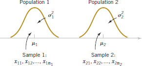
FIGURE 10-1 Two independent populations.
When statistical significance is observed in a randomized experiment, the experimenter can be confident in the conclusion that the difference in treatments resulted in the difference in response. That is, we can be confident that a cause-and-effect relationship has been found.
Sometimes the objects to be used in the comparison are not assigned at random to the treatments. For example, the September 1992 issue of Circulation (a medical journal published by the American Heart Association) reports a study linking high iron levels in the body with increased risk of heart attack. The study, done in Finland, tracked 1931 men for five years and showed a statistically significant effect of increasing iron levels on the incidence of heart attacks. In this study, the comparison was not performed by randomly selecting a sample of men and then assigning some to a “low iron level” treatment and the others to a “high iron level” treatment. The researchers just tracked the subjects over time. Recall from Chapter 1 that this type of study is called an observational study.
It is difficult to identify causality in observational studies because the observed statistically significant difference in response for the two groups may be due to some other underlying factor (or group of factors) that was not equalized by randomization and not due to the treatments. For example, the difference in heart attack risk could be attributable to the difference in iron levels or to other underlying factors that form a reasonable explanation for the observed results—such as cholesterol levels or hypertension.
In this section, we consider statistical inferences on the difference in means μ1 − μ2 of two normal distributions where the variances ![]() and
and ![]() are known. The assumptions for this section are summarized as follows.
are known. The assumptions for this section are summarized as follows.
Assumptions for Two-Sample Inference
(1) X11, X12,..., X1n1 is a random sample from population 1.
(2) X21, X22,..., X2n2 is a random sample from population 2.
(3) The two populations represented by X1 and X2 are independent.
(4) Both populations are normal.
A logical point estimator of μ1 − μ2 is the difference in sample means ![]() 1 −
1 − ![]() 2. Based on the properties of expected values,
2. Based on the properties of expected values,
![]()
and the variance of ![]() 1 −
1 − ![]() 2 is
2 is
![]()
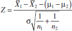
Based on the assumptions and the preceding results, we may state the following.
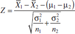
The quantity
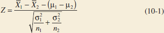
has a N(0,1) distribution.
This result will be used to develop procedures for tests of hypotheses and to construct confidence intervals on μ1 − μ2. Essentially, we may think of μ1 − μ2 as a parameter θ where estimator is ![]() =
= ![]() 1 −
1 − ![]() 2 with variance
2 with variance ![]() =
= ![]() /n1 +
/n1 + ![]() /n2. If θ0 is the null hypothesis value specified for θ, the test statistic will be (
/n2. If θ0 is the null hypothesis value specified for θ, the test statistic will be (![]() − θ0)/
− θ0)/![]() . Notice how similar this is to the test statistic for a single mean used in Equation 9-8 of Chapter 9.
. Notice how similar this is to the test statistic for a single mean used in Equation 9-8 of Chapter 9.
10-1.1 HYPOTHESIS TESTS ON THE DIFFERENCE IN MEANS, VARIANCES KNOWN
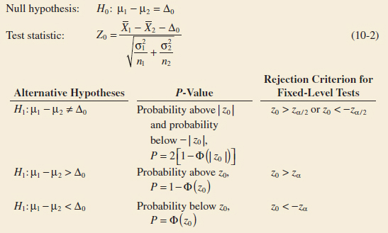
We now consider hypothesis testing on the difference in the means μ1 − μ2 of two normal populations. Suppose that we are interested in testing whether the difference in means μ1 − μ2 is equal to a specified value Δ0. Thus, the null hypothesis will be stated as H0: μ1 − μ2 = Δ0 Obviously, in many cases, we will specify Δ0 = 0 so that we are testing the equality of two means (i.e., H0: μ1 = μ2). The appropriate test statistic would be found by replacing μ1 − μ2 in Equation 10-1 by Δ0: this test statistic would have a standard normal distribution under H0. That is, the standard normal distribution is the reference distribution for the test statistic. Suppose that the alternative hypothesis is H1: μ1 − μ2 ≠ Δ0. A sample value of ![]() 1 −
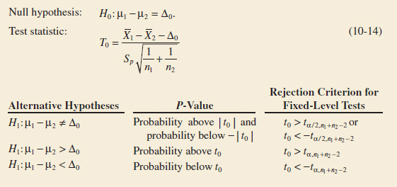
1 − ![]() 2 that is considerably different from Δ0 is evidence that H1 is true. Because Z0 has the N(0,1) distribution when H0 is true, we would calculate the P-value as the sum of the probabilities beyond the test statistic value z0 and −z0 in the standard normal distribution. That is, P = 2[1 − Φ(|z0|)]. This is exactly what we did in the one-sample z-test of Section 4-4.1. If we wanted to perform a fixed-significance-level test, we would take −zα/2 and zα/2 as the boundaries of the critical region just as we did in the single-sample z-test. This would give a test with level of significance α. P-values or critical regions for the one-sided alternatives would be determined similarly. Formally, we summarize these results in the following display.
2 that is considerably different from Δ0 is evidence that H1 is true. Because Z0 has the N(0,1) distribution when H0 is true, we would calculate the P-value as the sum of the probabilities beyond the test statistic value z0 and −z0 in the standard normal distribution. That is, P = 2[1 − Φ(|z0|)]. This is exactly what we did in the one-sample z-test of Section 4-4.1. If we wanted to perform a fixed-significance-level test, we would take −zα/2 and zα/2 as the boundaries of the critical region just as we did in the single-sample z-test. This would give a test with level of significance α. P-values or critical regions for the one-sided alternatives would be determined similarly. Formally, we summarize these results in the following display.
Tests on the Difference in Means, Variances Known
Example 10-1 Paint Drying Time A product developer is interested in reducing the drying time of a primer paint. Two formulations of the paint are tested; formulation 1 is the standard chemistry, and formulation 2 has a new drying ingredient that should reduce the drying time. From experience, it is known that the standard deviation of drying time is 8 minutes, and this inherent variability should be unaffected by the addition of the new ingredient. Ten specimens are painted with formulation 1, and another 10 specimens are painted with formulation 2; the 20 specimens are painted in random order. The two sample average drying times are ![]() 1 = 121 minutes and
1 = 121 minutes and ![]() 2 = 112 minutes, respectively. What conclusions can the product developer draw about the effectiveness of the new ingredient, using α = 0.05?
2 = 112 minutes, respectively. What conclusions can the product developer draw about the effectiveness of the new ingredient, using α = 0.05?
We apply the seven-step procedure to this problem as follows:
- Parameter of interest: The quantity of interest is the difference in mean drying times, μ1 − μ2, and Δ0 = 0.
- Non hypothesis: H0:μ1 − μ2 = 0, or H0:μ1 = μ2.
- Alternative hypothesis: H1: μ1 > μ2. We want to reject H0 if the new ingredient reduces mean drying time.
- Test statistic: The test statistic is
- Reject H0 if: Reject H0: μ1 = μ2 if the P-value is less than 0.05.
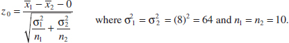
- Computations: Because
 1 = 121 minutes and 2 = 112 minutes, the test statistic is
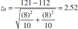
- Conclusion: Because z0 = 2.52, the P-value is P = 1 − Φ(2.52) = 0.0059, so we reject H0 at the α = 0.05 level.
Practical Interpretation: We conclude that adding the new ingredient to the paint significantly reduces the drying time. This is a strong conclusion.
When the population variances are unknown, the sample variances ![]() and
and ![]() can be substituted into the test statistic Equation 10-2 to produce a large-sample test for the difference in means. This procedure will also work well when the populations are not necessarily normally distributed. However, both n1 and n2 should exceed 40 for this large-sample test to be valid.
can be substituted into the test statistic Equation 10-2 to produce a large-sample test for the difference in means. This procedure will also work well when the populations are not necessarily normally distributed. However, both n1 and n2 should exceed 40 for this large-sample test to be valid.
10-1.2 TYPE II ERROR AND CHOICE OF SAMPLE SIZE
Use of Operating Characteristic Curves
The operating characteristic (OC) curves in Appendix Charts VIIa, VIIb, VIIc, and VIId may be used to evaluate the type II error probability for the hypotheses in the display (10-2). These curves are also useful in determining sample size. Curves are provided for α = 0.05 and α = 0.01. For the two-sided alternative hypothesis, the abscissa scale of the operating characteristic curve in charts VIIa and VIIb is d, where
![]()
and one must choose equal sample sizes, say, n = n1 = n2. The one-sided alternative hypotheses require the use of Charts VIIc and VIId. For the one-sided alternatives H1:μ1 − μ2 > Δ0 or H1:μ1 − μ2 < Δ0, the abscissa scale is also given by
![]()
It is not unusual to encounter problems where the costs of collecting data differ substantially for the two populations or when the variance for one population is much greater than the other. In those cases, we often use unequal sample sizes. If n1 ≠ n2, the operating characteristic curves may be entered with an equivalent value of n computed from
![]()
If n1 ≠ n2 and their values are fixed in advance, Equation 10-4 is used directly to calculate n, and the operating characteristic curves are entered with a specified d to obtain β. If we are given d and it is necessary to determine n1 and n2 to obtain a specified β, say, β*, we guess at trial values of n1 and n2, calculate n in Equation 10-4, and enter the curves with the specified value of d to find β. If β = β*, the trial values of n1 and n2 are satisfactory. If β ≠ β*, adjustments to n1 and n2 are made and the process is repeated.
Example 10-2 Paint Drying Time, Sample Size from OC Curves Consider the paint drying time experiment from Example 10-1. If the true difference in mean drying times is as much as 10 minutes, find the sample sizes required to detect this difference with probability at least 0.90.
The appropriate value of the abscissa parameter is (because Δ0 = 0, and Δ = 10)
![]()
and because the detection probability or power of the test must be at least 0.9, with α = 0.05, we find from Appendix Chart VIIc that n = n1 = n2 ![]() 11.
11.
Sample Size Formulas
It is also possible to obtain formulas for calculating the sample sizes directly. Suppose that the null hypothesis H0: μ1 − μ2 = Δ0 is false and that the true difference in means is μ1 − μ2 = Δ where Δ > Δ0. One may find formulas for the sample size required to obtain a specific value of the type II error probability β for a given difference in means Δ and level of significance α.
For example, we first write the expression for the β-error for the two-sided alternative, which is
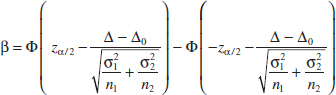
The derivation for sample size closely follows the single-sample case in Section 9-2.2.
Sample Size for a Two-Sided Test on the Difference in Means with n1 = n2, Variances Known
For the two-sided alternative hypothesis with significance level α, the sample size n1 = n2 = n required to detect a true difference in means of Δ with power at least 1 − β is
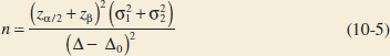
This approximation is valid when ![]() is small compared to β.
is small compared to β.
For a one-sided alternative hypothesis with significance level α, the sample size n1 = n2 = n required to detect a true difference in means of Δ(≠ Δ0) with power at least 1 − β is
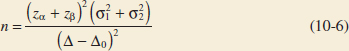
where Δ is the true difference in means of interest. Then by following a procedure similar to that used to obtain Equation 9-17, the expression for β can be obtained for the case where n = n1 = n2.
Example 10-3 Paint Drying Time Sample Size To illustrate the use of these sample size equations, consider the situation described in Example 10-1, and suppose that if the true difference in drying times is as much as 10 minutes, we want to detect this with probability at least 0.90. Under the null hypothesis, Δ0 = 0. We have a one-sided alternative hypothesis with Δ = 10, α = 0.05 (so zα = z0.05 = 1.645), and because the power is 0.9, β = 0.10 (so zβ = z0.10 = 1.28). Therefore, we may find the required sample size from Equation 10-6 as follows:
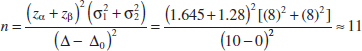
This is exactly the same as the result obtained from using the OC curves.
10-1.3 CONFIDENCE INTERVAL ON THE DIFFERENCE IN MEANS, VARIANCES KNOWN
The 100(1 − α)% confidence interval on the difference in two means μ1 − μ2 when the variances are known can be found directly from results given previously in this section. Recall that X11, X12,..., X1n1 is a random sample of n1 observations from the first population and X21, X22,..., X2n2 is a random sample of n2 observations from the second population. The difference in sample means ![]() 1 −
1 − ![]() 2 is a point estimator of μ1 − μ2, and
2 is a point estimator of μ1 − μ2, and
has a standard normal distribution if the two populations are normal or is approximately standard normal if the conditions of the central limit theorem apply, respectively. This implies that P(−zα/2 ≤ Z ≤ zα/2) = 1 − α, or
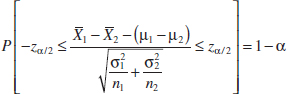
This can be rearranged as
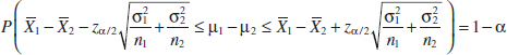
Therefore, the 100(1 − α)% confidence interval for μ1 − μ2 is defined as follows.
Confidence Interval on the Difference in Means, Variances Known
If ![]() 1 and
1 and ![]() 2 are the means of independent random samples of sizes n1 and n2 from two independent normal populations with known variances
2 are the means of independent random samples of sizes n1 and n2 from two independent normal populations with known variances ![]() and
and ![]() , respectively, a 100(1 − α)% confidence interval (CI) for μ1 − μ2 is
, respectively, a 100(1 − α)% confidence interval (CI) for μ1 − μ2 is
![]()
where zα/2 is the upper α/2 percentage point of the standard normal distribution.
The confidence level 1 − α is exact when the populations are normal. For nonnormal populations, the confidence level is approximately valid for large sample sizes.
Equation 10-7 can also be used as a large sample CI on the difference in mean when ![]() and
and ![]() are unknown by substituting
are unknown by substituting ![]() and
and ![]() for the population variances. For this to be a valid procedure, both sample sizes n1 and n2 should exceed 40.
for the population variances. For this to be a valid procedure, both sample sizes n1 and n2 should exceed 40.
Example 10-4 Aluminum Tensile Strength Tensile strength tests were performed on two different grades of aluminum spars used in manufacturing the wing of a commercial transport aircraft. From past experience with the spar manufacturing process and the testing procedure, the standard deviations of tensile strengths are assumed to be known. The data obtained are as follows: n1 = 10, ![]() 1 = 87.6, σ1 = 1, n2 = 12,
1 = 87.6, σ1 = 1, n2 = 12, ![]() 2 = 74.5, and σ2 = 1.5. If μ1 and μ2 denote the true mean tensile strengths for the two grades of spars, we may find a 90% on the difference in mean strength μ1 − μ2 as follows:
2 = 74.5, and σ2 = 1.5. If μ1 and μ2 denote the true mean tensile strengths for the two grades of spars, we may find a 90% on the difference in mean strength μ1 − μ2 as follows:
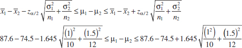
Therefore, the 90% confidence interval on the difference in mean tensile strength (in kilograms per square millimeter) is
![]()
Practical Interpretation: Notice that the confidence interval does not include zero, implying that the mean strength of aluminum grade 1 (μ1) exceeds the mean strength of aluminum grade 2 (μ2). In fact, we can state that we are 90% confident that the mean tensile strength of aluminum grade 1 exceeds that of aluminum grade 2 by between 12.22 and 13.98 kilograms per square millimeter.
Choice of Sample Size
If the standard deviations σ1 and σ2 are known (at least approximately) and the two sample sizes n1 and n2 are equal (n1 = n2 = n, say), we can determine the sample size required so that the error in estimating μ1 − μ2 by ![]() 1 −
1 − ![]() 2 will be less than E at 100(1 − α)% confidence. The required sample size from each population is
2 will be less than E at 100(1 − α)% confidence. The required sample size from each population is
Sample Size for a Confidence Interval on the Difference in Means, Variances Known

Remember to round up if n is not an integer. This ensures that the level of confidence does not drop below 100(1 − α)%.
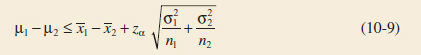
One-Sided Confidence Bounds
One-sided confidence bounds on μ1 − μ2 may also be obtained. A 100(1 − α)% upper-confidence bound on μ1 − μ2 is
One-Sided Upper-Confidence Bound
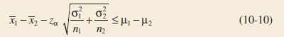
and a 100(1 − α)% lower-confidence bound is
One-Sided Lower-Confidence Bound
Exercises FOR SECTION 10-1
![]() Problem available in WileyPLUS at instructor's discretion.
Problem available in WileyPLUS at instructor's discretion.
![]() Go Tutorial Tutoring problem available in WileyPLUS at instructor's discretion.
Go Tutorial Tutoring problem available in WileyPLUS at instructor's discretion.
10-1. ![]() Consider the hypothesis test H0: μ1 = μ2 against H1: μ1 ≠ μ2 with known variances σ1 = 10 and σ2 = 5. Suppose that sample sizes n1 = 10 and n2 = 15 and that
Consider the hypothesis test H0: μ1 = μ2 against H1: μ1 ≠ μ2 with known variances σ1 = 10 and σ2 = 5. Suppose that sample sizes n1 = 10 and n2 = 15 and that ![]() 1 = 4.7 and
1 = 4.7 and ![]() 2 = 7.8. Use α = 0.05.
2 = 7.8. Use α = 0.05.
(a) Test the hypothesis and find the P-value.
(b) Explain how the test could be conducted with a confidence interval.
(c) What is the power of the test in part (a) for a true difference in means of 3?
(d) Assume that sample sizes are equal. What sample size should be used to obtain β = 0.05 if the true difference in means is 3? Assume that α = 0.05.
10-2. ![]() Consider the hypothesis test H0: μ1 = μ2 against H1: μ1 < μ2 with known variances σ1 = 10 and σ2 = 5. Suppose that sample sizes n1 = 10 and n2 = 15 and that
Consider the hypothesis test H0: μ1 = μ2 against H1: μ1 < μ2 with known variances σ1 = 10 and σ2 = 5. Suppose that sample sizes n1 = 10 and n2 = 15 and that ![]() 1 = 14.2 and
1 = 14.2 and ![]() 2 = 19.7. Use α = 0.05.
2 = 19.7. Use α = 0.05.
(a) Test the hypothesis and find the P-value.
(b) Explain how the test could be conducted with a confidence interval.
(c) What is the power of the test in part (a) if μ1 is 4 units less than μ2?
(d) Assume that sample sizes are equal. What sample size should be used to obtain β = 0.05 if μ1 is 4 units less than μ2? Assume that α = 0.05.
10-3. ![]() Consider the hypothesis test H0: μ1 = μ2 against H1: μ1 > μ2 with known variances σ1 = 10 and σ2 = 5. Suppose that sample sizes n1 = 10 and n2 = 15 and that
Consider the hypothesis test H0: μ1 = μ2 against H1: μ1 > μ2 with known variances σ1 = 10 and σ2 = 5. Suppose that sample sizes n1 = 10 and n2 = 15 and that ![]() 1 = 24.5 and
1 = 24.5 and ![]() 2 = 21.3. Use α = 0.01.
2 = 21.3. Use α = 0.01.
(a) Test the hypothesis and find the P-value.
(b) Explain how the test could be conducted with a confidence interval.
(c) What is the power of the test in part (a) if μ1 is 2 units greater than μ2?
(d) Assume that sample sizes are equal. What sample size should be used to obtain β = 0.05 if μ1 is 2 units greater than μ2? Assume that α = 0.05.
10-4. Two machines are used for filling plastic bottles with a net volume of 16.0 ounces. The fill volume can be assumed to be normal with standard deviation σ1 = 0.020 and σ2 = 0.025 ounces. A member of the quality engineering staff suspects that both machines fill to the same mean net volume, whether or not this volume is 16.0 ounces. A random sample of 10 bottles is taken from the output of each machine.
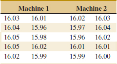
(a) Do you think the engineer is correct? Use α = 0.05. What is the P-value for this test?
(b) Calculate a 95% confidence interval on the difference in means. Provide a practical interpretation of this interval.
(c) What is the power of the test in part (a) for a true difference in means of 0.04?
(d) Assume that sample sizes are equal. What sample size should be used to ensure that β = 0.05 if the true difference in means is 0.04? Assume that α = 0.05.
10-5. ![]() Two types of plastic are suitable for an electronics component manufacturer to use. The breaking strength of this plastic is important. It is known that σ1 = σ2 = 1.0 psi. From a random sample of size n1 = 10 and n2 = 12, you obtain
Two types of plastic are suitable for an electronics component manufacturer to use. The breaking strength of this plastic is important. It is known that σ1 = σ2 = 1.0 psi. From a random sample of size n1 = 10 and n2 = 12, you obtain ![]() 1 = 162.5 and
1 = 162.5 and ![]() 2 = 155.0. The company will not adopt plastic 1 unless its mean breaking strength exceeds that of plastic 2 by at least 10 psi.
2 = 155.0. The company will not adopt plastic 1 unless its mean breaking strength exceeds that of plastic 2 by at least 10 psi.
(a) Based on the sample information, should it use plastic 1? Use α = 0.05 in reaching a decision. Find the P-value.
(b) Calculate a 95% confidence interval on the difference in means. Suppose that the true difference in means is really 12 psi.
(c) Find the power of the test assuming that α = 0.05.
(d) If it is really important to detect a difference of 12 psi, are the sample sizes employed in part (a) adequate in your opinion?
10-6. ![]() The burning rates of two different solid-fuel propellants used in air crew escape systems are being studied. It is known that both propellants have approximately the same standard deviation of burning rate; that is σ1 = σ2 = 3 centimeters per second. Two random samples of n1 = 20 and n2 = 20 specimens are tested; the sample mean burning rates are
The burning rates of two different solid-fuel propellants used in air crew escape systems are being studied. It is known that both propellants have approximately the same standard deviation of burning rate; that is σ1 = σ2 = 3 centimeters per second. Two random samples of n1 = 20 and n2 = 20 specimens are tested; the sample mean burning rates are ![]() 1 = 18 centimeters per second and
1 = 18 centimeters per second and ![]() 2 = 24 centimeters per second.
2 = 24 centimeters per second.
(a) Test the hypothesis that both propellants have the same mean burning rate. Use α = 0.05. What is the P-value?
(b) Construct a 95% confidence interval on the difference in means μ1 − μ2. What is the practical meaning of this interval?
(c) What is the β-error of the test in part (a) if the true difference in mean burning rate is 2.5 centimeters per second?
(d) Assume that sample sizes are equal. What sample size is needed to obtain power of 0.9 at a true difference in means of 14 cm/s?
10-7. ![]() Two different formulations of an oxygenated motor fuel are being tested to study their road octane numbers. The variance of road octane number for formulation 1 is
Two different formulations of an oxygenated motor fuel are being tested to study their road octane numbers. The variance of road octane number for formulation 1 is ![]() = 1.5, and for formulation, 2 it is
= 1.5, and for formulation, 2 it is ![]() = 1.2. Two random samples of size n1 = 15 and n2 = 20 are tested, and the mean road octane numbers observed are
= 1.2. Two random samples of size n1 = 15 and n2 = 20 are tested, and the mean road octane numbers observed are ![]() 1 = 89.6 and
1 = 89.6 and ![]() 2 = 92.5. Assume normality.
2 = 92.5. Assume normality.
(a) If formulation 2 produces a higher road octane number than formulation 1, the manufacturer would like to detect it. Formulate and test an appropriate hypothesis using α = 0.05. What is the P-value?
(b) Explain how the question in part (a) could be answered with a 95% confidence interval on the difference in mean road octane number.
(c) What sample size would be required in each population if you wanted to be 95% confident that the error in estimating the difference in mean road octane number is less than 1?
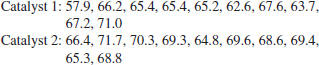
10-8. A polymer is manufactured in a batch chemical process. Viscosity measurements are normally made on each batch, and long experience with the process has indicated that the variability in the process is fairly stable with σ = 20. Fifteen batch viscosity measurements are given as follows:
![]()
A process change that involves switching the type of catalyst used in the process is made. Following the process change, eight batch viscosity measurements are taken:
![]()
Assume that process variability is unaffected by the catalyst change. If the difference in mean batch viscosity is 10 or less, the manufacturer would like to detect it with a high probability.
(a) Formulate and test an appropriate hypothesis using α = 0.10. What are your conclusions? Find the P-value.
(b) Find a 90% confidence interval on the difference in mean batch viscosity resulting from the process change.
(c) Compare the results of parts (a) and (b) and discuss your findings.
10-9. ![]() The concentration of active ingredient in a liquid laundry detergent is thought to be affected by the type of catalyst used in the process. The standard deviation of active concentration is known to be 3 grams per liter regardless of the catalyst type. Ten observations on concentration are taken with each catalyst, and the data follow:
The concentration of active ingredient in a liquid laundry detergent is thought to be affected by the type of catalyst used in the process. The standard deviation of active concentration is known to be 3 grams per liter regardless of the catalyst type. Ten observations on concentration are taken with each catalyst, and the data follow:
(a) Find a 95% confidence interval on the difference in mean active concentrations for the two catalysts. Find the P-value.
(b) Is there any evidence to indicate that the mean active concentrations depend on the choice of catalyst? Base your answer on the results of part (a).
(c) Suppose that the true mean difference in active concentration is 5 grams per liter. What is the power of the test to detect this difference if α = 0.05?
(d) If this difference of 5 grams per liter is really important, do you consider the sample sizes used by the experimenter to be adequate? Does the assumption of normality seem reasonable for both samples?
10-10. An article in Industrial Engineer (September 2012) reported on a study of potential sources of injury to equine veterinarians conducted at a university veterinary hospital. Forces on the hand were measured for several common activities that veterinarians engage in when examining or treating horses. We will consider the forces on the hands for two tasks, lifting and using ultrasound. Assume that both sample sizes are 6, the sample mean force for lifting was 6.0 pounds with standard deviation 1.5 pounds, and the sample mean force for using ultrasound was 6.2 pounds with standard deviation 0.3 pounds (data read from graphs in the article). Assume that the standard deviations are known. Is there evidence to conclude that the two activities result in significantly different forces on the hands?
10-11. Reconsider the data from Exercise 10-10. Find a 95% confidence interval on the difference in mean force on the hands for the two activities. How would you interpret this CI? Is the value zero in the CI? What connection does this have with the conclusion that you reached in Exercise 10-10?
10-12. Reconsider the study described in Exercise 10-10. Suppose that you wanted to detect a true difference in mean force of 0.25 pounds on the hands for these two activities. What level of type II error would you recommend here? What sample size would be required?
10-13. In their book Statistical Thinking (2nd ed.), Roger Hoerl and Ron Snee provide data on the absorbency of paper towels that were produced by two different manufacturing processes. From process 1, the sample size was 10 and had a mean and standard deviation of 190 and 15, respectively. From process 2, the sample size was 4 with a mean and standard deviation of 310 and 50, respectively. Is there evidence to support a claim that the mean absorbency of the towels from process 2 have higher mean absorbency than the towels from process 1? Assume that the standard deviations are known. What level of type I error would you consider appropriate for this problem?
10-2 Inference on the Difference in Means of two Normal Distributions, Variances Unknown
We now extend the results of the previous section to the difference in means of the two distributions in Fig. 10-1 when the variances of both distributions ![]() and
and ![]() are unknown. If the sample sizes n1 and n2 exceed 40, the normal distribution procedures in Section 10-1 could be used. However, when small samples are taken, we will assume that the populations are normally distributed and base our hypotheses tests and confidence intervals on the t distribution. This nicely parallels the case of inference on the mean of a single sample with unknown variance.
are unknown. If the sample sizes n1 and n2 exceed 40, the normal distribution procedures in Section 10-1 could be used. However, when small samples are taken, we will assume that the populations are normally distributed and base our hypotheses tests and confidence intervals on the t distribution. This nicely parallels the case of inference on the mean of a single sample with unknown variance.
10-2.1 HYPOTHESES TESTS ON THE DIFFERENCE IN MEANS, VARIANCES UNKNOWN
We now consider tests of hypotheses on the difference in means μ1 − μ2 of two normal distributions where the variances ![]() and
and ![]() are unknown. A t-statistic will be used to test these hypotheses. As noted earlier and in Section 9-3, the normality assumption is required to develop the test procedure, but moderate departures from normality do not adversely affect the procedure. Two different situations must be treated. In the first case, we assume that the variances of the two normal distributions are unknown but equal; that is,
are unknown. A t-statistic will be used to test these hypotheses. As noted earlier and in Section 9-3, the normality assumption is required to develop the test procedure, but moderate departures from normality do not adversely affect the procedure. Two different situations must be treated. In the first case, we assume that the variances of the two normal distributions are unknown but equal; that is, ![]() =
= ![]() = σ2. In the second, we assume that
= σ2. In the second, we assume that ![]() and
and ![]() are unknown and not necessarily equal.
are unknown and not necessarily equal.
Case 1:  =
=  = σ2
= σ2
Suppose that we have two independent normal populations with unknown means μ1 and μ2, and unknown but equal variances, ![]() =
= ![]() = σ2. We wish to test
= σ2. We wish to test
![]()
Let X11, X12,..., X1n1 be a random sample of n1 observations from the first population and X21, X22,..., X2n2 be a random sample of n2 observations from the second population. Let ![]() 1,
1, ![]() 2,
2, ![]() , and
, and ![]() be the sample means and sample variances, respectively. Now the expected value of the difference in sample means
be the sample means and sample variances, respectively. Now the expected value of the difference in sample means ![]() 1 −
1 − ![]() 2 is E(
2 is E(![]() 1 −
1 − ![]() 2) = μ1 − μ2, so
2) = μ1 − μ2, so ![]() 1 −
1 − ![]() 2 is an unbiased estimator of the difference in means. The variance of
2 is an unbiased estimator of the difference in means. The variance of ![]() 1 −
1 − ![]() 2 is
2 is
![]()
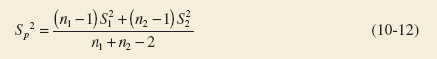
It seems reasonable to combine the two sample variances ![]() and
and ![]() to form an estimator of σ2. The pooled estimator of σ2 is defined as follows.
to form an estimator of σ2. The pooled estimator of σ2 is defined as follows.
Pooled Estimator of Variance
The pooled estimator of σ2, denoted by ![]() , is defined by
, is defined by
It is easy to see that the pooled estimator ![]() can be written as
can be written as
![]()
where 0 < w ≤ 1. Thus, ![]() is a weighted average of the two sample variances
is a weighted average of the two sample variances ![]() and
and ![]() where the weights w and 1 − w depend on the two sample sizes n1 and n2. Obviously, if n1 = n2 = n, w = 0.5,
where the weights w and 1 − w depend on the two sample sizes n1 and n2. Obviously, if n1 = n2 = n, w = 0.5, ![]() is just the arithmetic average of
is just the arithmetic average of ![]() and
and ![]() . If n1 = 10 and n2 = 20 (say), w = 0.32 and 1 − w = 0.68. The first sample contributes n1 − 1 degrees of freedom to
. If n1 = 10 and n2 = 20 (say), w = 0.32 and 1 − w = 0.68. The first sample contributes n1 − 1 degrees of freedom to ![]() and the second sample contributes n2 − 1 degrees of freedom. Therefore,
and the second sample contributes n2 − 1 degrees of freedom. Therefore, ![]() has n1 + n2 − 2 degrees of freedom.
has n1 + n2 − 2 degrees of freedom.
has a N(0, 1) distribution. Replacing σ by Sp gives the following.
Given the assumptions of this section, the quantity
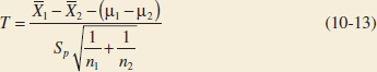
has a t distribution with n1 + n2 − 2 degrees of freedom.
The use of this information to test the hypotheses in Equation 10-11 is now straightforward: Simply replace μ1 − μ2 by Δ0, and the resulting test statistic has a t distribution with n1 + n2 − 2 degrees of freedom under H0: μ1 − μ2 = Δ0. Therefore, the reference distribution for the test statistic is the t distribution with n1 + n2 − 2 degrees of freedom. The calculation of P-values and the location of the critical region for fixed-significance-level testing for both two- and one-sided alternatives parallels those in the one-sample case. Because a pooled estimate of variance is used, the procedure is often called the Pooled t-test.
Tests on the Difference in Means of Two Normal Distributions, Variances Unknown and Equal*
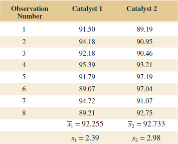
Example 10-5 Yield from a Catalyst Two catalysts are being analyzed to determine how they affect the mean yield of a chemical process. Specifically, catalyst 1 is currently used; but catalyst 2 is acceptable. Because catalyst 2 is cheaper, it should be adopted, if it does not change the process yield. A test is run in the pilot plant and results in the data shown in Table 10-1. Figure 10-2 presents a normal probability plot and a comparative box plot of the data from the two samples. Is there any difference in the mean yields? Use α = 0.05, and assume equal variances.
![]() TABLE • 10-1 Catalyst Yield Data, Example 10-5
TABLE • 10-1 Catalyst Yield Data, Example 10-5
The solution using the seven-step hypothesis-testing procedure is as follows:
- Parameter of interest: The parameters of interest are μ1 and μ2, the mean process yield using catalysts 1 and 2, respectively, and we want to know if μ1 − μ2 = 0.
- Null hypothesis: H0: μ1 − μ2 = 0, or H0: μ1 = μ2
- Alternative hypothesis: H1: μ1 ≠ μ2
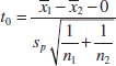
- Test statistic: The test statistic is
- Reject H0 if: Reject H0 if the P-value is less than 0.05.
- Computations: From Table 10-1, we have 1 = 92.255, s1 = 2.39, n1 = 8, 2 = 92.733, s2 = 2.98, and n2 = 8. Therefore
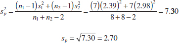
and
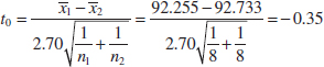
- Conclusions: Because |t0| = 0.35, we find from Appendix Table V that t0.40,14 = 0.258 and t0.25,14 = 0.692. Therefore, because 0.258 < 0.35 < 0.692, we conclude that lower and upper bounds on the P-value are 0.50 < P < 0.80. Therefore, because the P-value exceeds α = 0.05, the null hypothesis cannot be rejected.
Practical Interpretation: At the 0.05 level of significance, we do not have strong evidence to conclude that catalyst 2 results in a mean yield that differs from the mean yield when catalyst 1 is used.
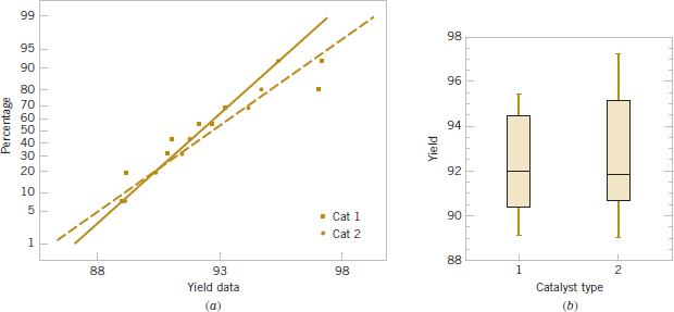
FIGURE 10-2 Normal probability plot and comparative box plot for the catalyst yield data in Example 10-5. (a) Normal probability plot. (b) Box plots.
Typical computer output for the two-sample t-test and confidence interval procedure for Example 10-5 follows:
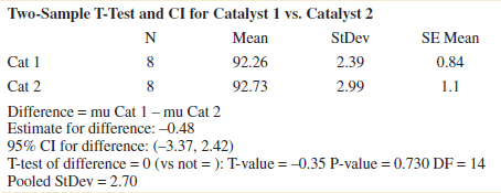
Notice that the numerical results are essentially the same as the manual computations in Example 10-5. The P-value is reported as P = 0.73. The two-sided CI on μ1 − μ2 is also reported. We will give the computing formula for the CI in Section 10-2.3. Figure 10-2 shows the normal probability plot of the two samples of yield data and comparative box plots. The normal probability plots indicate that there is no problem with the normality assumption or with the assumption of equal variances. Furthermore, both straight lines have similar slopes, providing some verification of the assumption of equal variances. The comparative box plots indicate that there is no obvious difference in the two catalysts although catalyst 2 has slightly more sample variability.
Case 2:  ≠
≠ 
In some situations, we cannot reasonably assume that the unknown variances ![]() and
and ![]() are equal. There is not an exact t-statistic available for testing H0: μ1 − μ2 = Δ0 in this case. However, an approximate result can be applied.
are equal. There is not an exact t-statistic available for testing H0: μ1 − μ2 = Δ0 in this case. However, an approximate result can be applied.
Case 2: Test Statistic for the Difference in Means, Variances Unknown and Not Assumed Equal
If H0: μ1 − μ2 = Δ0 is true, the statistic
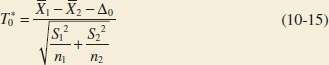
is distributed approximately as t with degrees of freedom given by
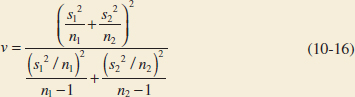
If v is not an integer, round down to the nearest integer.
Therefore, if ![]() ≠
≠ ![]() , the hypotheses on differences in the means of two normal distributions are tested as in the equal variances case except that
, the hypotheses on differences in the means of two normal distributions are tested as in the equal variances case except that ![]() is used as the test statistic and n1 + n2 − 2 is replaced by v in determining the degrees of freedom for the test.
is used as the test statistic and n1 + n2 − 2 is replaced by v in determining the degrees of freedom for the test.
The pooled t-test is very sensitive to the assumption of equal variances (so is the CI procedure in section 10-2.3). The two-sample t-test assuming that ![]() ≠
≠ ![]() is a safer procedure unless one is very sure about the equal variance assumption.
is a safer procedure unless one is very sure about the equal variance assumption.
Example 10-6 Arsenic in Drinking Water Arsenic concentration in public drinking water supplies is a potential health risk. An article in the Arizona Republic (May 27, 2001) reported drinking water arsenic concentrations in parts per billion (ppb) for 10 metropolitan Phoenix communities and 10 communities in rural Arizona. The data follow:
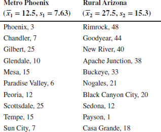
We wish to determine whether any difference exists in mean arsenic concentrations for metropolitan Phoenix communities and for communities in rural Arizona. Figure 10-3 shows a normal probability plot for the two samples of arsenic concentration. The assumption of normality appears quite reasonable, but because the slopes of the two straight lines are very different, it is unlikely that the population variances are the same.
Applying the seven-step procedure gives the following:
- Parameter of interest: The parameters of interest are the mean arsenic concentrations for the two geographic regions, say, μ1 and μ2, and we are interested in determining whether μ1 − μ2 = 0.
- Null hypothesis: H0: μ1 − μ2 = 0, or H0: μ1 − μ2
- Alternative hypothesis: H1: μ1 ≠ μ2
- Test statistic: The test statistic is

FIGURE 10-3 Normal probability plot of the arsenic concentration data from Example 10-6.
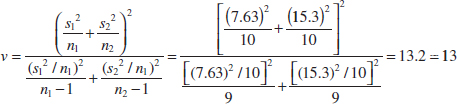
- Reject H0 if: The degrees of freedom on
 are found from Equation 10-16 as
Therefore, using α = 0.05 and a fixed-significance-level test, we would reject H0: μ1 = μ2 if
 > t0.025,13 = 2.160 or if
  < −t0.025,13 = −2.160.
 - Computations: Using the sample data, we find
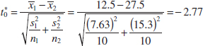
- Conclusion: Because
 = −2.77 < t0.025,13 = −2.160, we reject the null hypothesis.
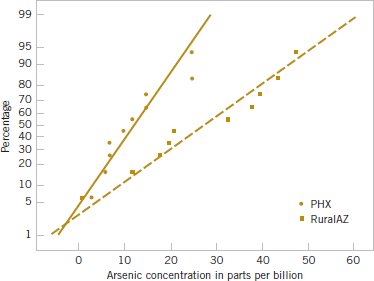
Practical Interpretation: There is strong evidence to conclude that mean arsenic concentration in the drinking water in rural Arizona is different from the mean arsenic concentration in metropolitan Phoenix drinking water. Furthermore, the mean arsenic concentration is higher in rural Arizona communities. The P-value for this test is approximately P = 0.016.
Typical computer output for this example follows:
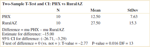
The computer-generated numerical results exactly match the calculations from Example 10-6. Note that a two-sided 95% CI on μ1 − μ2 is also reported. We will discuss its computation in Section 10-2.3; however, note that the interval does not include zero. Indeed, the upper 95% of confidence limit is −3.29 ppb, well below zero, and the mean observed difference is ![]() 1 −
1 − ![]() 2 = 12.5−27.5 = −15 ppb.
2 = 12.5−27.5 = −15 ppb.
Example 10-7 Chocolate and Cardiovascular Health An article in Nature (2003, Vol. 48, p. 1013) described an experiment in which subjects consumed different types of chocolate to determine the effect of eating chocolate on a measure of cardiovascular health. We will consider the results for only dark chocolate and milk chocolate. In the experiment, 12 subjects consumed 100 grams of dark chocolate and 200 grams of milk chocolate, one type of chocolate per day, and after one hour, the total antioxidant capacity of their blood plasma was measures in an assay. The subjects consisted of seven women and five men with an average age range of 32.2 ±1 years, an average weight of 65.8 ± 3.1 kg, and average body mass index of 21.9 ± 0.4 kg/m2. Data similar to that reported in the article follows.
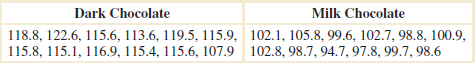
Is there evidence to support the claim that consuming dark chocolate produces a higher mean level of total blood plasma antioxidant capacity than consuming milk chocolate? Let μ1 be the mean blood plasma antioxidant capacity resulting from eating dark chocolate and μ2 be the mean blood plasma antioxidant capacity resulting from eating milk chocolate. The hypotheses that we wish to test are
![]()
The results of applying the pooled t-test to this experiment are as follows:
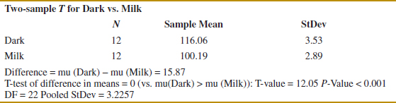
Because the P-value is so small (< 0.001), the null hypothesis would be rejected. Strong evidence supports the claim that consuming dark chocolate produces a higher mean level of total blood plasma antioxidant capacity than consuming milk chocolate.
10-2.2 TYPE II ERROR AND CHOICE OF SAMPLE SIZE
The operating characteristic curves in Appendix Charts VIIe, VIIf, VIIg, and VIIh are used to evaluate the type II error for the case in which ![]() =
= ![]() = σ2. Unfortunately, when
= σ2. Unfortunately, when ![]() ≠
≠ ![]() , the distribution of
, the distribution of ![]() is unknown if the null hypothesis is false, and no operating characteristic curves are available for this case.
is unknown if the null hypothesis is false, and no operating characteristic curves are available for this case.
For the two-sided alternative H1: μ1 − μ2 = Δ ≠ Δ0, when ![]() =
= ![]() = σ2 and n1 = n2 = n, Charts VIIe and VIIf are used with
= σ2 and n1 = n2 = n, Charts VIIe and VIIf are used with
![]()
where Δ is the true difference in means that is of interest. To use these curves, they must be entered with the sample size n* = 2n − 1. For the one-sided alternative hypothesis, we use Charts VIIg and VIIh and define d and Δ as in Equation 10-17. It is noted that the parameter d is a function of σ, which is unknown. As in the single-sample t-test, we may have to rely on a prior estimate of σ or use a subjective estimate. Alternatively, we could define the differences in the mean that we wish to detect relative to σ.
Example 10-8 Yield from Catalyst Sample Size Consider the catalyst experiment in Example 10-5. Suppose that, if catalyst 2 produces a mean yield that differs from the mean yield of catalyst 1 by 4.0%, we would like to reject the null hypothesis with probability at least 0.85. What sample size is required?
Using sp = 2.70 as a rough estimate of the common standard deviation σ, we have d = |Δ|/2σ = |4.0|/[(2)(2.70)] = 0.74. From Appendix Chart VIIe with d = 0.74 and β = 0.15, we find n* = 20, approximately. Therefore, because n* = 2n − 1,
![]()
and we would use sample sizes of n1 = n2 = n = 11.
Many software packages perform power and sample size calculations for the two-sample t-test (equal variances). Typical output from Example 10-8 is as follows:
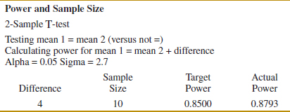
The results agree fairly closely with the results obtained from the OC curve.
10-2.3 CONFIDENCE INTERVAL ON THE DIFFERENCE IN MEANS, VARIANCES UNKNOWN
Case 1:  =
=  = σ2
= σ2
To develop the confidence interval for the difference in means μ1 − μ2 when both variances are equal, note that the distribution of the statistic
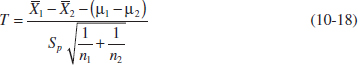
is the t distribution with n1 + n2 − 2 degrees of freedom. Therefore P(−tα/2,n1 + n2−2 ≤ T ≤ tα/2,n1+n2−2) = 1 − α. Now substituting Equation 10-18 for T and manipulating the quantities inside the probability statement will lead to the 100(1 − α)% confidence interval on μ1 − μ2.
If ![]() 1,
1, ![]() 2,
2, ![]() , and
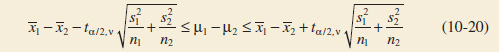
, and ![]() are the sample means and variances of two random samples of sizes n1 and n2, respectively, from two independent normal populations with unknown but equal variances, a 100(1 − α)% confidence interval on the difference in means μ1 − μ2 is
are the sample means and variances of two random samples of sizes n1 and n2, respectively, from two independent normal populations with unknown but equal variances, a 100(1 − α)% confidence interval on the difference in means μ1 − μ2 is
![]()
where sp = ![]() is the pooled estimate of the common population standard deviation, and tα/2,n1+n2−2 is the upper α/2 percentage point of the t distribution with n1 + n2 − 2 degrees of freedom.
is the pooled estimate of the common population standard deviation, and tα/2,n1+n2−2 is the upper α/2 percentage point of the t distribution with n1 + n2 − 2 degrees of freedom.
Example 10-9 Cement Hydration An article in the journal Hazardous Waste and Hazardous Materials (1989, Vol. 6) reported the results of an analysis of the weight of calcium in standard cement and cement doped with lead. Reduced levels of calcium would indicate that the hydration mechanism in the cement is blocked and would allow water to attack various locations in the cement structure. Ten samples of standard cement had an average weight percent calcium of ![]() 1 = 90.0 with a sample standard deviation of s1 = 5.0, and 15 samples of the lead-doped cement had an average weight percent calcium of
1 = 90.0 with a sample standard deviation of s1 = 5.0, and 15 samples of the lead-doped cement had an average weight percent calcium of ![]() 2 = 87.0 with a sample standard deviation of s2 = 4.0.
2 = 87.0 with a sample standard deviation of s2 = 4.0.
We will assume that weight percent calcium is normally distributed and find a 95% confidence interval on the difference in means, μ1 − μ2, for the two types of cement. Furthermore, we will assume that both normal populations have the same standard deviation.
The pooled estimate of the common standard deviation is found using Equation 10-12 as follows:
![]()
Therefore, the pooled standard deviation estimate is sp = ![]() = 4.4. The 95% confidence interval is found using Equation 10-19:
= 4.4. The 95% confidence interval is found using Equation 10-19:
![]()
or upon substituting the sample values and using t0.025,23 = 2.069,
![]()
which reduces to
![]()
Practical Interpretation: Notice that the 95% confidence interval includes zero; therefore, at this level of confidence we cannot conclude that there is a difference in the means. Put another way, there is no evidence that doping the cement with lead affected the mean weight percent of calcium; therefore, we cannot claim that the presence of lead affects this aspect of the hydration mechanism at the 95% level of confidence.
Case 2:  =
= 
In many situations, assuming that ![]() =
= ![]() is not reasonable. When this assumption is unwarranted, we may still find a 100(1 − α)% confidence interval on μ1 − μ2 using the fact that T* = [
is not reasonable. When this assumption is unwarranted, we may still find a 100(1 − α)% confidence interval on μ1 − μ2 using the fact that T* = [![]() 1 −
1 − ![]() 2 − (μ1 − μ2)]/
2 − (μ1 − μ2)]/![]() is distributed approximately as t with degrees of freedom v given by Equation 10-16. The CI expression follows.
is distributed approximately as t with degrees of freedom v given by Equation 10-16. The CI expression follows.
Case 2: Approximate Confidence Interval on the Difference in Means, Variances Unknown and not Assumed Equal
If ![]() 1,
1, ![]() 2,
2, ![]() , and
, and ![]() are the means and variances of two random samples of sizes n1 and n2, respectively, from two independent normal populations with unknown and unequal variances, an approximate 100(1 − α)% confidence interval on the difference in means μ1 − μ2 is
are the means and variances of two random samples of sizes n1 and n2, respectively, from two independent normal populations with unknown and unequal variances, an approximate 100(1 − α)% confidence interval on the difference in means μ1 − μ2 is
where v is given by Equation 10-16 and tα/2,ν is the upper α/2 percentage point of the t distribution with v degrees of freedom.
Exercises FOR SECTION 10-2
![]() Problem available in WileyPLUS at instructor's discretion.
Problem available in WileyPLUS at instructor's discretion.
![]() Go Tutorial Tutoring problem available in WileyPLUS at instructor's discretion.
Go Tutorial Tutoring problem available in WileyPLUS at instructor's discretion.
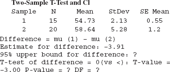
10-14. Consider the following computer output.
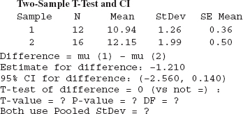
(a) Fill in the missing values. Is this a one-sided or a two-sided test? Use lower and upper bounds for the P-value.
(b) What are your conclusions if α = 0.05? What if α = 0.01?
(c) This test was done assuming that the two population variances were equal. Does this seem reasonable?
(d) Suppose that the hypothesis had been H0: μ1 = μ2 versus H0: μ1 < μ2. What would your conclusions be if α = 0.05?
10-15. Consider the computer output below.
(a) Fill in the missing values. Is this a one-sided or a two-sided test? Use lower and upper bounds for the P-value.
(b) What are your conclusions if α = 0.05? What if α = 0.01?
(c) This test was done assuming that the two population variances were different. Does this seem reasonable?
(d) Suppose that the hypotheses had been H0: μ1 = μ2 versus H0: μ1 ≠ μ2. What would your conclusions be if α = 0.05?
10-16. ![]() Consider the hypothesis test H0: μ1 = μ2 against H1: μ1 ≠ μ2. Suppose that sample sizes are n1 = 15 and n2 = 15, that
Consider the hypothesis test H0: μ1 = μ2 against H1: μ1 ≠ μ2. Suppose that sample sizes are n1 = 15 and n2 = 15, that ![]() 1 = 4.7 and
1 = 4.7 and ![]() 2 = 7.8, and that
2 = 7.8, and that ![]() = 4 and
= 4 and ![]() = 6.25. Assume that
= 6.25. Assume that ![]() =
= ![]() and that the data are drawn from normal distributions. Use α = 0.05.
and that the data are drawn from normal distributions. Use α = 0.05.
(a) Test the hypothesis and find the P-value.
(b) Explain how the test could be conducted with a confidence interval.
(c) What is the power of the test in part (a) for a true difference in means of 3?
(d) Assume that sample sizes are equal. What sample size should be used to obtain β = 0.05 if the true difference in means is −2? Assume that α = 0.05.
10-17. ![]() Consider the hypothesis test H0: μ1 = μ2 against H1: μ1 = μ2. Suppose that sample sizes n1 = 15 and n2 = 15, that
Consider the hypothesis test H0: μ1 = μ2 against H1: μ1 = μ2. Suppose that sample sizes n1 = 15 and n2 = 15, that ![]() 1 = 6.2 and
1 = 6.2 and ![]() 2 = 7.8, and that
2 = 7.8, and that ![]() = 4 and
= 4 and ![]() = 6.25. Assume that
= 6.25. Assume that ![]() =
= ![]() and that the data are drawn from normal distributions. Use α = 0.05.
and that the data are drawn from normal distributions. Use α = 0.05.
(a) Test the hypothesis and find the P-value.
(b) Explain how the test could be conducted with a confidence interval.
(c) What is the power of the test in part (a) if μ1 is 3 units less than μ2?
(d) Assume that sample sizes are equal. What sample size should be used to obtain β = 0.05 if μ1 is 2.5 units less than μ2? Assume that α = 0.05.
10-18. ![]() Consider the hypothesis test H0: μ1 = μ2 against H1: μ1 ≠ μ2. Suppose that sample sizes n1 = 10 and n2 = 10, that
Consider the hypothesis test H0: μ1 = μ2 against H1: μ1 ≠ μ2. Suppose that sample sizes n1 = 10 and n2 = 10, that ![]() 1 = 7.8 and
1 = 7.8 and ![]() 2 = 5.6, and that
2 = 5.6, and that ![]() = 4 and
= 4 and ![]() = 9. Assume that
= 9. Assume that ![]() =
= ![]() and that the data are drawn from normal distributions. Use α = 0.05.
and that the data are drawn from normal distributions. Use α = 0.05.
(a) Test the hypothesis and find the P-value.
(b) Explain how the test could be conducted with a confidence interval.
(c) What is the power of the test in part (a) if μ1 is 3 units greater than μ2?
(d) Assume that sample sizes are equal. What sample size should be used to obtain β = 0.05 if μ1 is 3 units greater than μ2? Assume that α = 0.05.
10-19. ![]() Go Tutorial The diameter of steel rods manufactured on two different extrusion machines is being investigated. Two random samples of sizes n1 = 15 and n1 = 17 are selected, and the sample means and sample variances are
Go Tutorial The diameter of steel rods manufactured on two different extrusion machines is being investigated. Two random samples of sizes n1 = 15 and n1 = 17 are selected, and the sample means and sample variances are ![]() 1 = 8.73,
1 = 8.73, ![]() = 0.35,
= 0.35, ![]() 2 = 8.68, and
2 = 8.68, and ![]() = 0.40, respectively. Assume that
= 0.40, respectively. Assume that ![]() =
= ![]() and that the data are drawn from a normal distribution.
and that the data are drawn from a normal distribution.
(a) Is there evidence to support the claim that the two machines produce rods with different mean diameters? Use α = 0.05 in arriving at this conclusion. Find the P-value.
(b) Construct a 95% confidence interval for the difference in mean rod diameter. Interpret this interval.
10-20. An article in Fire Technology investigated two different foam-expanding agents that can be used in the nozzles of fire-fighting spray equipment. A random sample of five observations with an aqueous film-forming foam (AFFF) had a sample mean of 4.7 and a standard deviation of 0.6. A random sample of five observations with alcohol-type concentrates (ATC) had a sample mean of 6.9 and a standard deviation 0.8.
(a) Can you draw any conclusions about differences in mean foam expansion? Assume that both populations are well represented by normal distributions with the same standard deviations.
(b) Find a 95% confidence interval on the difference in mean foam expansion of these two agents.
10-21. ![]() Two catalysts may be used in a batch chemical process. Twelve batches were prepared using catalyst 1, resulting in an average yield of 86 and a sample standard deviation of 3. Fifteen batches were prepared using catalyst 2, and they resulted in an average yield of 89 with a standard deviation of 2. Assume that yield measurements are approximately normally distributed with the same standard deviation.
Two catalysts may be used in a batch chemical process. Twelve batches were prepared using catalyst 1, resulting in an average yield of 86 and a sample standard deviation of 3. Fifteen batches were prepared using catalyst 2, and they resulted in an average yield of 89 with a standard deviation of 2. Assume that yield measurements are approximately normally distributed with the same standard deviation.
(a) Is there evidence to support a claim that catalyst 2 produces a higher mean yield than catalyst 1? Use α = 0.01.
(b) Find a 99% confidence interval on the difference in mean yields that can be used to test the claim in part (a).
10-22. The deflection temperature under load for two different types of plastic pipe is being investigated. Two random samples of 15 pipe specimens are tested, and the deflection temperatures observed are as follows (in °F):
Type 1: 206, 188, 205, 187, 194, 193, 207, 185, 189, 213, 192, 210, 194, 178, 205
Type 2: 177, 197, 206, 201, 180, 176, 185, 200, 197, 192, 198, 188, 189, 203, 192
(a) Construct box plots and normal probability plots for the two samples. Do these plots provide support of the assumptions of normality and equal variances? Write a practical interpretation for these plots.
(b) Do the data support the claim that the deflection temperature under load for type 1 pipe exceeds that of type 2? In reaching your conclusions, use α = 0.05. Calculate a P-value.
(c) If the mean deflection temperature for type 1 pipe exceeds that of type 2 by as much as 5°F, it is important to detect this difference with probability at least 0.90. Is the choice of n1 = n2 = 15 adequate? Use α = 0.05.
10-23. ![]() In semiconductor manufacturing, wet chemical etching is often used to remove silicon from the backs of wafers prior to metallization. The etch rate is an important characteristic in this process and known to follow a normal distribution. Two different etching solutions have been compared using two random samples of 10 wafers for each solution. The observed etch rates are as follows (in mils per minute):
In semiconductor manufacturing, wet chemical etching is often used to remove silicon from the backs of wafers prior to metallization. The etch rate is an important characteristic in this process and known to follow a normal distribution. Two different etching solutions have been compared using two random samples of 10 wafers for each solution. The observed etch rates are as follows (in mils per minute):
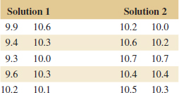
(a) Construct normal probability plots for the two samples. Do these plots provide support for the assumptions of normality and equal variances? Write a practical interpretation for these plots.
(b) Do the data support the claim that the mean etch rate is the same for both solutions? In reaching your conclusions, use α = 0.05 and assume that both population variances are equal. Calculate a P-value.
(c) Find a 95% confidence interval on the difference in mean etch rates.
10-24. ![]() Two suppliers manufacture a plastic gear used in a laser printer. The impact strength of these gears measured in foot-pounds is an important characteristic. A random sample of 10 gears from supplier 1 results in
Two suppliers manufacture a plastic gear used in a laser printer. The impact strength of these gears measured in foot-pounds is an important characteristic. A random sample of 10 gears from supplier 1 results in ![]() 1 = 290 and s1 = 12, and another random sample of 16 gears from the second supplier results in
1 = 290 and s1 = 12, and another random sample of 16 gears from the second supplier results in ![]() 2 = 321 and s2 = 22.
2 = 321 and s2 = 22.
(a) Is there evidence to support the claim that supplier 2 provides gears with higher mean impact strength? Use α = 0.05, and assume that both populations are normally distributed but the variances are not equal. What is the P-value for this test?
(b) Do the data support the claim that the mean impact strength of gears from supplier 2 is at least 25 foot-pounds higher than that of supplier 1? Make the same assumptions as in part (a).
(c) Construct a confidence interval estimate for the difference in mean impact strength, and explain how this interval could be used to answer the question posed regarding supplier-to-supplier differences.
10-25. ![]() The melting points of two alloys used in formulating solder were investigated by melting 21 samples of each material. The sample mean and standard deviation for alloy 1 was
The melting points of two alloys used in formulating solder were investigated by melting 21 samples of each material. The sample mean and standard deviation for alloy 1 was ![]() 1 = 420°F and s1 = 4°F, and for alloy 2, they were
1 = 420°F and s1 = 4°F, and for alloy 2, they were ![]() 2 = 426°F and s2 = 3°F.
2 = 426°F and s2 = 3°F.
(a) Do the sample data support the claim that both alloys have the same melting point? Use α = 0.05 and assume that both populations are normally distributed and have the same standard deviation. Find the P-value for the test.
(b) Suppose that the true mean difference in melting points is 3°F. How large a sample would be required to detect this difference using an α = 0.05 level test with probability at least 0.9? Use σ1 = σ2 = 4 as an initial estimate of the common standard deviation.
10-26. ![]() A photoconductor film is manufactured at a nominal thickness of 25 mils. The product engineer wishes to increase the mean speed of the film and believes that this can be achieved by reducing the thickness of the film to 20 mils. Eight samples of each film thickness are manufactured in a pilot production process, and the film speed (in microjoules per square inch) is measured. For the 25-mil film, the sample data result is
A photoconductor film is manufactured at a nominal thickness of 25 mils. The product engineer wishes to increase the mean speed of the film and believes that this can be achieved by reducing the thickness of the film to 20 mils. Eight samples of each film thickness are manufactured in a pilot production process, and the film speed (in microjoules per square inch) is measured. For the 25-mil film, the sample data result is ![]() 1 = 1.15 and s1 = 0.11, and for the 20-mil film the data yield
1 = 1.15 and s1 = 0.11, and for the 20-mil film the data yield ![]() 2 = 1.06 and s2 = 0.09. Note that an increase in film speed would lower the value of the observation in microjoules per square inch.
2 = 1.06 and s2 = 0.09. Note that an increase in film speed would lower the value of the observation in microjoules per square inch.
(a) Do the data support the claim that reducing the film thickness increases the mean speed of the film? Use σ = 0.10, and assume that the two population variances are equal and the underlying population of film speed is normally distributed. What is the P-value for this test?
(b) Find a 95% confidence interval on the difference in the two means that can be used to test the claim in part (a).
10-27. ![]() Two companies manufacture a rubber material intended for use in an automotive application. The part will be subjected to abrasive wear in the field application, so you decide to compare the material produced by each company in a test. Twenty-five samples of material from each company are tested in an abrasion test, and the amount of wear after 1000 cycles is observed. For company 1, the sample mean and standard deviation of wear are
Two companies manufacture a rubber material intended for use in an automotive application. The part will be subjected to abrasive wear in the field application, so you decide to compare the material produced by each company in a test. Twenty-five samples of material from each company are tested in an abrasion test, and the amount of wear after 1000 cycles is observed. For company 1, the sample mean and standard deviation of wear are ![]() 1 = 20 milligrams/1000 cycles and s1 = 2 milligrams/1000 cycles, and for company 2, you obtain
1 = 20 milligrams/1000 cycles and s1 = 2 milligrams/1000 cycles, and for company 2, you obtain ![]() 2 = 15 milligrams/1000 cycles and s2 = 8 milligrams/1000 cycles.
2 = 15 milligrams/1000 cycles and s2 = 8 milligrams/1000 cycles.
(a) Do the data support the claim that the two companies produce material with different mean wear? Use α = 0.05, and assume that each population is normally distributed but that their variances are not equal. What is the P-value for this test?
(b) Do the data support a claim that the material from company 1 has higher mean wear than the material from company 2? Use the same assumptions as in part (a).
(c) Construct confidence intervals that will address the questions in parts (a) and (b) above.
10-28. ![]() The thickness of a plastic film (in mils) on a substrate material is thought to be influenced by the temperature at which the coating is applied. In completely randomized experiment, 11 substrates are coated at 125°F, resulting in a sample mean coating thickness of
The thickness of a plastic film (in mils) on a substrate material is thought to be influenced by the temperature at which the coating is applied. In completely randomized experiment, 11 substrates are coated at 125°F, resulting in a sample mean coating thickness of ![]() 1 = 103.5 and a sample standard deviation of s1 = 10.2. Another 13 substrates are coated at 150°F for which
1 = 103.5 and a sample standard deviation of s1 = 10.2. Another 13 substrates are coated at 150°F for which ![]() 2 = 99.7 and s2 = 20.1 are observed. It was originally suspected that raising the process temperature would reduce mean coating thickness.
2 = 99.7 and s2 = 20.1 are observed. It was originally suspected that raising the process temperature would reduce mean coating thickness.
(a) Do the data support this claim? Use α = 0.01 and assume that the two population standard deviations are not equal. Calculate an approximate P-value for this test.
(b) How could you have answered the question posed regarding the effect of temperature on coating thickness by using a confidence interval? Explain your answer.
10-29. ![]() An article in Electronic Components and Technology Conference (2001, Vol. 52, pp. 1167–1171) compared single versus dual spindle saw processes for copper metallized wafers. A total of 15 devices of each type were measured for the width of the backside chipouts,
An article in Electronic Components and Technology Conference (2001, Vol. 52, pp. 1167–1171) compared single versus dual spindle saw processes for copper metallized wafers. A total of 15 devices of each type were measured for the width of the backside chipouts, ![]() single = 66.385, ssingle = 7.895 and
single = 66.385, ssingle = 7.895 and ![]() double = 45.278, sdouble = 8.612.
double = 45.278, sdouble = 8.612.
(a) Do the sample data support the claim that both processes have the same chip outputs? Use α = 0.05 and assume that both populations are normally distributed and have the same variance. Find the P-value for the test.
(b) Construct a 95% two-sided confidence interval on the mean difference in spindle saw process. Compare this interval to the results in part (a).
(c) If the β-error of the test when the true difference in chip outputs is 15 should not exceed 0.1, what sample sizes must be used? Use α = 0.05.
10-30. An article in IEEE International Symposium on Electromagnetic Compatibility (2002, Vol. 2, pp. 667–670) quantified the absorption of electromagnetic energy and the resulting thermal effect from cellular phones. The experimental results were obtained from in vivo experiments conducted on rats. The arterial blood pressure values (mmHg) for the control group (8 rats) during the experiment are ![]() 1 = 90, s1 = 5 and for the test group (9 rats) are
1 = 90, s1 = 5 and for the test group (9 rats) are ![]() 2 = 115, s2 = 10.
2 = 115, s2 = 10.
(a) Is there evidence to support the claim that the test group has higher mean blood pressure? Use α = 0.05, and assume that both populations are normally distributed but the variances are not equal. What is the P-value for this test?
(b) Calculate a confidence interval to answer the question in part (a).
(c) Do the data support the claim that the mean blood pressure from the test group is at least 15 mmHg higher than the control group? Make the same assumptions as in these part (a).
(d) Explain how the question in part (c) could be answered with a confidence interval.
10-31. ![]() An article in Radio Engineering and Electronic Physics [1984, Vol. 29 No. (3), pp. 63–66] investigated the behavior of a stochastic generator in the presence of external noise. The number of periods was measured in a sample of 100 trains for each of two different levels of noise voltage, 100 and 150 mV. For 100 mV, the mean number of periods in a train was 7.9 with s = 2.6 For 150 mV, the mean was 6.9 with s = 2.4.
An article in Radio Engineering and Electronic Physics [1984, Vol. 29 No. (3), pp. 63–66] investigated the behavior of a stochastic generator in the presence of external noise. The number of periods was measured in a sample of 100 trains for each of two different levels of noise voltage, 100 and 150 mV. For 100 mV, the mean number of periods in a train was 7.9 with s = 2.6 For 150 mV, the mean was 6.9 with s = 2.4.
(a) It was originally suspected that raising noise voltage would reduce the mean number of periods. Do the data support this claim? Use α = 0.01 and assume that each population is normally distributed and the two population variances are equal. What is the P-value for this test?
(b) Calculate a confidence interval to answer the question in part (a).
10-32. An article in Technometrics (1999, Vol. 41, pp. 202–211) studied the capability of a gauge by measuring the weights of two sheets of paper. The data follow.
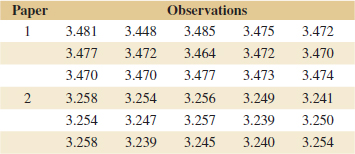
(a) Check the assumption that the data from each sheet are from normal distributions.
(b) Test the hypothesis that the mean weight of the two sheets is equal against the alternative that it is not (and assume equal variances). Use α = 0.05 and assume equal variances. Find the P-value.
(c) Repeat the previous test with α = 0.10.
(d) Compare your answers for parts (b) and (c) and explain why they are the same or different.
(e) Explain how the questions in parts (b) and (c) could be answered with confidence intervals.
10-33. ![]() The overall distance traveled by a golf ball is tested by hitting the ball with Iron Byron, a mechanical golfer with a swing that is said to emulate the distance hit by the legendary champion, Byron Nelson. Ten randomly selected balls of two different brands are tested and the overall distance measured. The data follow:
The overall distance traveled by a golf ball is tested by hitting the ball with Iron Byron, a mechanical golfer with a swing that is said to emulate the distance hit by the legendary champion, Byron Nelson. Ten randomly selected balls of two different brands are tested and the overall distance measured. The data follow:
Brand 1: 275, 286, 287, 271, 283, 271, 279, 275, 263, 267
Brand 2: 258, 244, 260, 265, 273, 281, 271, 270, 263, 268
(a) Is there evidence that overall distance is approximately normally distributed? Is an assumption of equal variances justified?
(b) Test the hypothesis that both brands of ball have equal mean overall distance. Use α = 0.05. What is the P-value?
(c) Construct a 95% two-sided CI on the mean difference in overall distance for the two brands of golf balls.
(d) What is the power of the statistical test in part (b) to detect a true difference in mean overall distance of 5 yards?
(e) What sample size would be required to detect a true difference in mean overall distance of 3 yards with power of approximately 0.75?
10-34. The “spring-like effect” in a golf club could be determined by measuring the coefficient of restitution (the ratio of the outbound velocity to the inbound velocity of a golf ball fired at the clubhead). Twelve randomly selected drivers produced by two clubmakers are tested and the coefficient of restitution measured. The data follow:
Club 1: 0.8406, 0.8104, 0.8234, 0.8198, 0.8235, 0.8562, 0.8123, 0.7976, 0.8184, 0.8265, 0.7773, 0.7871
Club 2: 0.8305, 0.7905, 0.8352, 0.8380, 0.8145, 0.8465, 0.8244, 0.8014, 0.8309, 0.8405, 0.8256, 0.8476
(a) Is there evidence that coefficient of restitution is approximately normally distributed? Is an assumption of equal variances justified?
(b) Test the hypothesis that both brands of clubs have equal mean coefficient of restitution. Use α = 0.05. What is the P-value of the test?
(c) Construct a 95% two-sided CI on the mean difference in coefficient of restitution for the two brands of golf clubs.
(d) What is the power of the statistical test in part (b) to detect a true difference in mean coefficient of restitution of 0.2?
(e) What sample size would be required to detect a true difference in mean coefficient of restitution of 0.1 with power of approximately 0.8?
10-35. Reconsider the paper towel absorbency data from Exercise 10-13. Find a 95% confidence interval on the difference in the towels' mean absorbency produced by the two processes. Assume the standard deviations are estimated from the data. How would you interpret this CI? Is the value zero in the CI?
10-36. European scientists sampled rivers in various seasons for chemical composition and algae growth (http://archive.ics.uci.edu/ml/datasets/Coil+1999+Competition+Data). The following is a random sample of 15 measurements from high-flow rivers and 13 from low-flow rivers of a total algae content (units are mg/L).
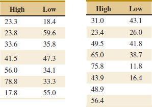
(a) Test the null hypothesis at α = 0.05, that the amount of algae content is the same in both high- and low-flow rivers. Is the alternative one or two sided?
(b) Find a 95% confidence interval for the difference in the mean algae content for the two flow rates.
(c) Is the value zero contained in the 95% confidence interval? Explain the connection with the conclusion you reached in part (a).
(d) Do box plots of algae content by flow rate show any violations of the assumptions for the tests and confidence interval that you performed?
10-37. Olympic swimmers are seeded according to their previous 12-month performances with faster swimmers going into the later heats. The last 24 swimmers, however, are distributed among the last three heats more evenly. So we should see large differences in times of heats one–five but not among the last three heats. The data of times from heats five–seven are in seconds for the 100m swim. NA indicates that the swimmer did not swim. Is there a statistically significant difference in the mean time of swimmers in heats 6 and 7 and the mean time of swimmers in heat 5?
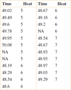
Is there evidence to suggest that the means of the heats differ for slower swimmers in heat five and the faster swimmers in heat seven? What about the means of the two sets of elite swimmers in heats six and seven? Use α = 0.05.
10-38. A paper in Quality Engineering [2013, Vol. 25(1)] presented data on cycles to failure of solder joints at different temperatures for different types of printed circuit boards (PCB). Failure data for two temperatures (20 and 60°C) for a copper-nickel-gold PCB follow.
![]()
(a) Test the null hypothesis at α = 0.05 that the cycles to failure are the same at both temperatures. Is the alternative one or two sided?
(b) Find a 95% confidence interval for the difference in the mean cycles to failure for the two temperatures.
(c) Is the value zero contained in the 95% confidence interval? Explain the connection with the conclusion you reached in part (a).
(d) Do normal probability plots of part cycles to failure indicate any violations of the assumptions for the tests and confidence interval that you performed?
10-39. An article in Polymer Degradation and Stability (2006, Vol. 91) presented data from a nine-year aging study on S537 foam. Foam samples were compressed to 50% of their original thickness and stored at different temperatures for nine years. At the start of the experiment as well as during each year, sample thickness was measured, and the thickness of the eight samples at each storage condition were recorded. The data for two storage conditions follow.
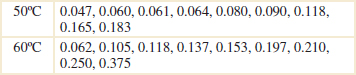
(a) Is there evidence to support the claim that mean compression increases with the temperature at the storage condition?
(b) Find a 95% confidence interval for the difference in the mean compression for the two temperatures.
(c) Is the value zero contained in the 95% confidence interval? Explain the connection with the conclusion you reached in part (a).
(d) Do normal probability plots of compression indicate any violations of the assumptions for the tests and confidence interval that you performed?
10-40. An article in Quality Engineering [2012, Vol. 24(1)] described an experiment on a grinding wheel. The following are some of the grinding force data (in N) from this experiment at two different vibration levels.
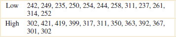
(a) Is there evidence to support the claim that the mean grinding force increases with the vibration level?
(b) Find a 95% confidence interval for the difference in the mean grinding force for the two vibration levels.
(c) Is the value zero contained in the 95% confidence interval? Explain the connection with the conclusion you reached in part (a).
(d) Do normal probability plots of grinding force indicate any violations of the assumptions for the tests and confidence interval that you performed?
10-3 A Nonparametric Test for the Difference in Two Means
Suppose that we have two independent continuous populations X1 and X2 with means μ1 and μ2, but we are unwilling to assume that they are (approximately) normal. However, we can assume that the distributions of X1 and X2 are continuous and have the same shape and spread, and differ only (possibly) in their locations. The Wilcoxon rank-sum test can be used to test the hypothesis H0: μ1 = μ2. This procedure is sometimes called the Mann-Whitney test, although the Mann-Whitney test statistic is usually expressed in a different form.
10-3.1 DESCRIPTION OF THE WILCOXON RANK-SUM TEST
Let X11, X12,..., X1n1 and X21, X22,..., X2n2 be two independent random samples of sizes n1 ≤ n2 from the continuous populations X1 and X2 described earlier. We wish to test the hypotheses
![]()
The test procedure is as follows. Arrange all n1 + n2 observations in ascending order of magnitude and assign ranks to them. If two or more observations are tied (identical), use the mean of the ranks that would have been assigned if the observations differed.
Let W1 be the sum of the ranks in the smaller sample (1), and define W2 to be the sum of the ranks in the other sample. Then,
![]()
Now if the sample means do not differ, we will expect the sum of the ranks to be nearly equal for both samples after adjusting for the difference in sample size. Consequently, if the sums of the ranks differ greatly, we will conclude that the means are not equal.
Appendix Table X contains the critical value of the rank sums for α = 0.05 and α = 0.01 assuming the preceding two-sided alternative. Refer to Appendix Table X with the appropriate sample sizes n1 and n2, and the critical value wα can be obtained. The null H0: μ1 = μ2 is rejected in favor of H1: μ1 < μ2, if either of the observed values w1 or w2 is less than or equal to the tabulated critical value wα.
The procedure can also be used for one-sided alternatives. If the alternative is H1: μ1 < μ2, reject H0 if w1 ≤ wα; for H1: μ1 > μ2, reject H0 if w2 ≤ wα. For these one-sided tests, the tabulated critical values wα correspond to levels of significance of α = 0.025 and α = 0.005.
Example 10-10 Axial Stress The mean axial stress in tensile members used in an aircraft structure is being studied. Two alloys are being investigated. Alloy 1 is a traditional material, and alloy 2 is a new aluminum-lithium alloy that is much lighter than the standard material. Ten specimens of each alloy type are tested, and the axial stress is measured. The sample data are assembled in Table 10-2. Using α = 0.05, we wish to test the hypothesis that the means of the two stress distributions are identical.
![]() TABLE • 10-2 Axial Stress for Two Aluminum-Lithium Alloys
TABLE • 10-2 Axial Stress for Two Aluminum-Lithium Alloys
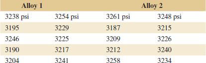
We will apply the seven-step hypothesis-testing procedure to this problem:
- Parameter of interest: The parameters of interest are the means of the two distributions of axial stress.
- Null hypothesis: H0: μ1 = μ2
- Alternative hypothesis: H1: μ1 ≠ μ2
- Test statistic: We will use the Wilcoxon rank-sum test statistic in Equation 10-21.
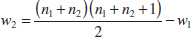
- Reject H0 if: Because α = 0.05 and n1 = n2 = 10, Appendix Table X gives the critical value as w0.05 = 78. If either w1 or w2 is less than or equal to w0.05 = 78, we will reject H0: μ1 = μ2.
- Computations: The data from Table 10-2 are arranged in ascending order and ranked as follows:
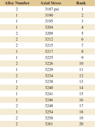
The sum of the ranks for alloy 1 is

and for alloy 2

- Conclusion: Because neither w1 nor w2 is less than or equal to w0.05 = 78, we cannot reject the null hypothesis that both alloys exhibit the same mean axial stress.
Practical Interpretation: The data do not demonstrate that there is a superior alloy for this particular application.
10-3.2 LARGE-SAMPLE APPROXIMATION
When both n1 and n2 are moderately large, say, more than eight, the distribution of w1 can be well approximated by the normal distribution with mean
![]()
and variance
![]()
Therefore, for n1 and n2 > 8, we could use
Normal Approximation for Wilcoxon Rank-Sum Test Statistic

as a statistic, and the appropriate critical region is |z0| > zα/2, z0 >zα, or z0 < − zα, depending on whether the test is a two-tailed, upper-tailed, or lower-tailed test.
10-3.3 COMPARISON TO THE t-TEST
In Chapter 9, we discussed the comparison of the t-test with the Wilcoxon signed-rank test. The results for the two-sample problem are similar to the one-sample case. That is, when the normality assumption is correct, the Wilcoxon rank-sum test is approximately 95% as efficient as the t-test in large samples. On the other hand, regardless of the form of the distributions, the Wilcoxon rank-sum test will always be at least 86% as efficient. The efficiency of the Wilcoxon test relative to the t-test is usually high if the underlying distribution has heavier tails than the normal, because the behavior of the t-test is very dependent on the sample mean, which is quite unstable in heavy-tailed distributions.
Exercises FOR SECTION 10-3
![]() Problem available in WileyPLUS at instructor's discretion.
Problem available in WileyPLUS at instructor's discretion.
![]() Go Tutorial Tutoring problem available in WileyPLUS at instructor's discretion.
Go Tutorial Tutoring problem available in WileyPLUS at instructor's discretion.
10-41. ![]() An electrical engineer must design a circuit to deliver the maximum amount of current to a display tube to achieve sufficient image brightness. Within her allowable design constraints, she has developed two candidate circuits and tests prototypes of each. The resulting data (in microamperes) are as follows:
An electrical engineer must design a circuit to deliver the maximum amount of current to a display tube to achieve sufficient image brightness. Within her allowable design constraints, she has developed two candidate circuits and tests prototypes of each. The resulting data (in microamperes) are as follows:
![]()
(a) Use the Wilcoxon rank-sum test to test H0: μ1 = μ2 against the alternative H1: μ1 > μ2. Use α = 0.025.
(b) Use the normal approximation for the Wilcoxon rank-sum test. Assume that α = 0.05. Find the approximate P-value for this test statistic.
10-42. ![]() One of the authors travels regularly to Seattle, Washington. He uses either Delta or Alaska airline. Flight delays are sometimes unavoidable, but he would be willing to give most of his business to the airline with the best on-time arrival record. The number of minutes that his flight arrived late for the last six trips on each airline follows. Is there evidence that either airline has superior on-time arrival performance? Use α = 0.01 and the Wilcoxon rank-sum test.
One of the authors travels regularly to Seattle, Washington. He uses either Delta or Alaska airline. Flight delays are sometimes unavoidable, but he would be willing to give most of his business to the airline with the best on-time arrival record. The number of minutes that his flight arrived late for the last six trips on each airline follows. Is there evidence that either airline has superior on-time arrival performance? Use α = 0.01 and the Wilcoxon rank-sum test.
![]()
10-43. ![]() The manufacturer of a hot tub is interested in testing two different heating elements for its product. The element that produces the maximum heat gain after 15 minutes would be preferable. The manufacturer obtains 10 samples of each heating unit and tests each one. The heat gain after 15 minutes (in °F) follows.
The manufacturer of a hot tub is interested in testing two different heating elements for its product. The element that produces the maximum heat gain after 15 minutes would be preferable. The manufacturer obtains 10 samples of each heating unit and tests each one. The heat gain after 15 minutes (in °F) follows.
![]()
(a) Is there any reason to suspect that one unit is superior to the other? Use α = 0.05 and the Wilcoxon rank-sum test.
(b) Use the normal approximation for the Wilcoxon rank-sum test. Assume that α = 0.05. What is the approximate P-value for this test statistic?
10-44. ![]() Go Tutorial Consider the chemical etch rate data in Exercise 10-23.
Go Tutorial Consider the chemical etch rate data in Exercise 10-23.
(a) Use the Wilcoxon rank-sum test to investigate the claim that the mean etch rate is the same for both solutions. If α = 0.05, what are your conclusions?
(b) Use the normal approximation for the Wilcoxon rank-sum test. Assume that α = 0.05. Find the approximate P-value for this test.
10-45. ![]() Consider the pipe deflection data in Exercise 10-22.
Consider the pipe deflection data in Exercise 10-22.
(a) Use the Wilcoxon rank-sum test for the pipe deflection temperature experiment. If α = 0.05, what are your conclusions?
(b) Use the normal approximation for the Wilcoxon rank-sum test. Assume that α = 0.05. Find the approximate P-value for this test.
10-46. Consider the distance traveled by a golf ball in Exercise 10-33.
(a) Use the Wilcoxon rank-sum test to investigate if the means differ. Use α = 0.05.
(b) Use the normal approximation for the Wilcoxon rank-sum test with α = 0.05. Find the approximate P-value for this test.
10-47. Another nonparametric test known as Tukey's quick test can be useful with two groups when one group has the minimum value overall (which we call the lower group) and the other (which we call the upper group) has the maximum. The Tukey test works by counting the “exceedences,” the number of observations in the lower group that are less than all the observations in the upper group plus the number in the upper group that are greater than all the observations in the lower group (count ties as 0.5). Call this number E. Then the test rejects the null hypothesis of equal means at α = 0.05 if E ≥ 7, at α = 0.01 if E ≥ 10, and at α = 0.001 if E ≥ 13.
Using the data from Exercise 10-36, see whether you come to the same conclusion about the null hypothesis.
10-48. Using the data from Exercise 10-37, test the hypotheses using Tukey's quick test and see whether you reach the same conclusions as you did for Exercise 10-37.
10-4 Paired t-Test
A special case of the two-sample t-tests of Section 10-2 occurs when the observations on the two populations of interest are collected in pairs. Each pair of observations, say (X1j, X2j), is taken under homogeneous conditions, but these conditions may change from one pair to another. For example, suppose that we are interested in comparing two different types of tips for a hardness-testing machine. This machine presses the tip into a metal specimen with a known force. By measuring the depth of the depression caused by the tip, the hardness of the specimen can be determined. If several specimens were selected at random, half tested with tip 1, half tested with tip 2, and the pooled or independent t-test in Section 10-2 was applied, the results of the test could be erroneous. The metal specimens could have been cut from bar stock that was produced in different heats, or they might not be homogeneous in some other way that might affect hardness. Then the observed difference in mean hardness readings for the two tip types also includes hardness differences in specimens.
A more powerful experimental procedure is to collect the data in pairs—that is, to make two hardness readings on each specimen, one with each tip. The test procedure would then consist of analyzing the differences in hardness readings on each specimen. If there is no difference between tips, the mean of the differences should be zero. This test procedure is called the paired t-test.
Let (X11, X21),(X12, X22),...,(X1n, X2n) be a set of n paired observations for which we assume that the mean and variance of the population represented by X1 are μ1 and ![]() , and the mean and variance of the population represented by X2 are μ2 and
, and the mean and variance of the population represented by X2 are μ2 and ![]() . Define the difference for each pair of observations as Dj = X1j − X2j, j = 1, 2,..., n. The Dj 's are assumed to be normally distributed with mean
. Define the difference for each pair of observations as Dj = X1j − X2j, j = 1, 2,..., n. The Dj 's are assumed to be normally distributed with mean
![]()
and variance ![]() , so testing hypotheses about the difference for μ1 and μ2 can be accomplished by performing a one-sample t-test on μD. Specifically, testing H0: μ1 − μ2 = Δ0 against H1: μ1 − μ2 ≠ Δ0 is equivalent to testing
, so testing hypotheses about the difference for μ1 and μ2 can be accomplished by performing a one-sample t-test on μD. Specifically, testing H0: μ1 − μ2 = Δ0 against H1: μ1 − μ2 ≠ Δ0 is equivalent to testing
![]()
The test statistic and decision procedure follow.
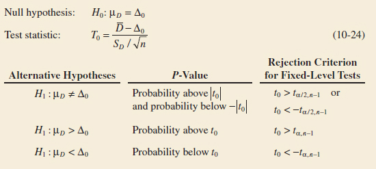
In Equation 10-24, ![]() is the sample average of the n differences D1, D2,..., Dn, and SD is the sample standard deviation of these differences.
is the sample average of the n differences D1, D2,..., Dn, and SD is the sample standard deviation of these differences.
Example 10-11 Shear Strength of Steel Girder An article in the Journal of Strain Analysis [1983, Vol. 18(2)] reports a comparison of several methods for predicting the shear strength for steel plate girders. Data for two of these methods, the Karlsruhe and Lehigh procedures, when applied to nine specific girders, are shown in Table 10-3. We wish to determine whether there is any difference (on the average) for the two methods.
The seven-step procedure is applied as follows:
- Parameter of interest: The parameter of interest is the difference in mean shear strength for the two methods—say, μD = μ1 − μ2 = 0.
- Null hypothesis: H0: μD = 0
- Alternative hypothesis: H1: μD ≠ 0
- Test statistic: The test statistic is

- Reject H0 if: Reject H0 if the P-value <0.05.
- Computations: The sample average and standard deviation of the differences dj are t0 = 6.08 and sd = 0.1350, and so the test statistic is
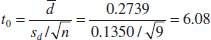
- Conclusion: Because t0.0005.8 = 5.041 and the value of the test statistic t0 = 6.15 exceeds this value, the P-value is less than 2(0.0005) = 0.001. Therefore, we conclude that the strength prediction methods yield different results.
Practical Interpretation: Specifically, the data indicate that the Karlsruhe method produces, on the average, greater strength predictions than does the Lehigh method. This is a strong conclusion.
Software can perform the paired t-test. Typical output for Example 10-10 follows:
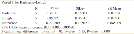
![]() TABLE • 10-3 Strength Predictions for Nine Steel Plate Girders (Predicted Load/Observed Load)
TABLE • 10-3 Strength Predictions for Nine Steel Plate Girders (Predicted Load/Observed Load)
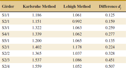
The results essentially agree with the manual calculations. In addition to the hypothesis test results. Most computer software report a two-sided CI on the difference in means. This Cl was found by constructing a single-sample CI on μD. We provide the details later.
Paired Versus Unpaired Comparisons
In performing a comparative experiment, the investigator can sometimes choose between the paired experiment and the two-sample (or unpaired) experiment. If n measurements are to be made on each population, the two-sample t-statistic is
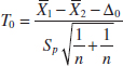
which would be compared to t2n−2, and of course, the paired t-statistic is
![]()
which is compared to tn−1. Notice that because
![]()
the numerators of both statistics are identical. However, the denominator of the two-sample t-test is based on the assumption that X1 and X2 are independent. In many paired experiments, a strong positive correlation ρ exists for X1 and X2. Then it can be shown that
![]()
assuming that both populations X1 and X2 have identical variances σ2. Furthermore, ![]() /n estimates the variance of
/n estimates the variance of ![]() . Whenever a positive correlation exists within the pairs, the denominator for the paired t-test will be smaller than the denominator of the two-sample t-test. This can cause the two-sample t-test to considerably understate the significance of the data if it is incorrectly applied to paired samples.
. Whenever a positive correlation exists within the pairs, the denominator for the paired t-test will be smaller than the denominator of the two-sample t-test. This can cause the two-sample t-test to considerably understate the significance of the data if it is incorrectly applied to paired samples.
Although pairing will often lead to a smaller value of the variance of ![]() 1 −
1 − ![]() 2, it does have a disadvantage—namely, the paired t-test leads to a loss of n − 1 degrees of freedom in comparison to the two-sample t-test. Generally, we know that increasing the degrees of freedom of a test increases the power against any fixed alternative values of the parameter.
2, it does have a disadvantage—namely, the paired t-test leads to a loss of n − 1 degrees of freedom in comparison to the two-sample t-test. Generally, we know that increasing the degrees of freedom of a test increases the power against any fixed alternative values of the parameter.
So how do we decide to conduct the experiment? Should we pair the observations or not? Although this question has no general answer, we can give some guidelines based on the preceding discussion.
- If the experimental units are relatively homogeneous (small σ) and the correlation within pairs is small, the gain in precision attributable to pairing will be offset by the loss of degrees of freedom, so an independent-sample experiment should be used.
- If the experimental units are relatively heterogeneous (large σ) and there is large positive correlation within pairs, the paired experiment should be used. Typically, this case occurs when the experimental units are the same for both treatments; as in Example 10-11, the same girders were used to test the two methods.
Implementing the rules still requires judgment because σ and ρ are never known precisely. Furthermore, if the number of degrees of freedom is large (say, 40 or 50), the loss of n − 1 of them for pairing may not be serious. However, if the number of degrees of freedom is small (say, 10 or 20), losing half of them is potentially serious if not compensated for by increased precision from pairing.
Confidence Interval for μD
To construct the confidence interval for μD = μ1 − μ2, note that
![]()
follows a t distribution with n − 1 degrees of freedom. Then, because P(−tα/2,n−1 ≤ T ≤ tα/2,n−1) = 1 − α, we can substitute for T in the preceding expression and perform the necessary steps to isolate μD = μ1 − μ2 for the inequalities. This leads to the following 100(1 − α)% confidence interval on μ1 − μ2.
Confidence Interval for μD from Paired Samples
If ![]() and sD are the sample mean and standard deviation of the difference of n random pairs of normally distributed measurements, a 100(1 − α)% confidence interval on the difference in means μD = μ1 − μ2 is
and sD are the sample mean and standard deviation of the difference of n random pairs of normally distributed measurements, a 100(1 − α)% confidence interval on the difference in means μD = μ1 − μ2 is
![]()
where tα/2,n−1 is the upper α/2% point of the t distribution with n − 1 degrees of freedom.
This confidence interval is also valid for the case in which ![]() ≠
≠ ![]() because
because ![]() estimates
estimates ![]() = V(X1 − X2). Also, for large samples (say, n ≥ 30 pairs), the explicit assumption of normality is unnecessary because of the central limit theorem.
= V(X1 − X2). Also, for large samples (say, n ≥ 30 pairs), the explicit assumption of normality is unnecessary because of the central limit theorem.
Example 10-12 Parallel Park Cars The journal Human Factors (1962, pp. 375–380) reported a study in which n = 14 subjects were asked to parallel park two cars having very different wheel bases and turning radii. The time in seconds for each subject was recorded and is given in Table 10-4. From the column of observed differences, we calculate ![]() = 1.21 and sD = 12.68. The 90% confidence interval for μD = μ1 − μ2 is found from Equation 10-25 as follows:
= 1.21 and sD = 12.68. The 90% confidence interval for μD = μ1 − μ2 is found from Equation 10-25 as follows:
![]() TABLE • 10-4 Time in Seconds to Parallel Park Two Automobiles
TABLE • 10-4 Time in Seconds to Parallel Park Two Automobiles
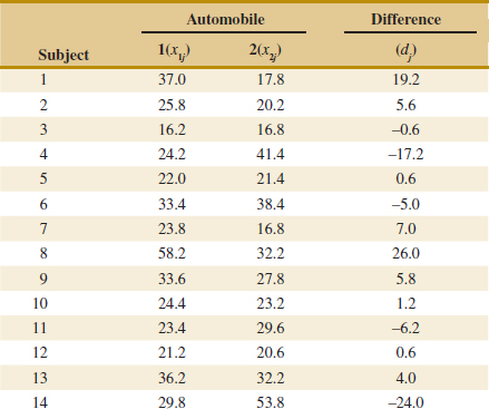
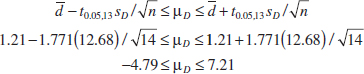
Notice that the confidence interval on μD includes zero. This implies that, at the 90% level of confidence, the data do not support the claim that the two cars have different mean parking times μ1 and μ2. That is, the value μD = μ1 − μ2 = 0 is not inconsistent with the observed data.
Nonparametric Approach to Paired Comparisons
Both the sign test and the Wilcoxon signed-rank test discussed in Section 9-9 can be applied to paired observations. In the case of the sign test, the null hypothesis is that the median of the differences is equal to zero (that is, H0: ![]() D= 0). The Wilcoxon signed-rank test is for the null hypothesis that the mean of the differences is equal to zero. The procedures are applied to the observed differences as described in Sections 9-9.1 and 9-9.2.
D= 0). The Wilcoxon signed-rank test is for the null hypothesis that the mean of the differences is equal to zero. The procedures are applied to the observed differences as described in Sections 9-9.1 and 9-9.2.
Exercises FOR SECTION 10-4
![]() Problem available in WileyPLUS at instructor's discretion.
Problem available in WileyPLUS at instructor's discretion.
![]() Go Tutorial Tutoring problem available in WileyPLUS at instructor's discretion.
Go Tutorial Tutoring problem available in WileyPLUS at instructor's discretion.
10-49. ![]() Consider the shear strength experiment described in Example 10-11.
Consider the shear strength experiment described in Example 10-11.
(a) Construct a 95% confidence interval on the difference in mean shear strength for the two methods. Is the result you obtained consistent with the findings in Example 10-11? Explain why.
(b) Do each of the individual shear strengths have to be normally distributed for the paired t-test to be appropriate, or is it only the difference in shear strengths that must be normal? Use a normal probability plot to investigate the normality assumption.
10-50. ![]() Consider the parking data in Example 10-12.
Consider the parking data in Example 10-12.
(a) Use the paired t-test to investigate the claim that the two types of cars have different levels of difficulty to parallel park. Use α = 0.10.
(b) Compare your results with the confidence interval constructed in Example 10-12 and comment on why they are the same or different.
(c) Investigate the assumption that the differences in parking times are normally distributed.
10-51. ![]() The manager of a fleet of automobiles is testing two brands of radial tires and assigns one tire of each brand at random to the two rear wheels of eight cars and runs the cars until the tires wear out. The data (in kilometers) follow. Find a 99% confidence interval on the difference in mean life. Which brand would you prefer based on this calculation?
The manager of a fleet of automobiles is testing two brands of radial tires and assigns one tire of each brand at random to the two rear wheels of eight cars and runs the cars until the tires wear out. The data (in kilometers) follow. Find a 99% confidence interval on the difference in mean life. Which brand would you prefer based on this calculation?
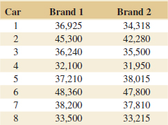
10-52. ![]() A computer scientist is investigating the usefulness of two different design languages in improving programming tasks. Twelve expert programmers who are familiar with both languages are asked to code a standard function in both languages and the time (in minutes) is recorded. The data follow:
A computer scientist is investigating the usefulness of two different design languages in improving programming tasks. Twelve expert programmers who are familiar with both languages are asked to code a standard function in both languages and the time (in minutes) is recorded. The data follow:

(a) Is the assumption that the difference in coding time is normally distributed reasonable?
(b) Find a 95% confidence interval on the difference in mean coding times. Is there any indication that one design language is preferable?
10-53. Fifteen adult males between the ages of 35 and 50 participated in a study to evaluate the effect of diet and exercise on blood cholesterol levels. The total cholesterol was measured in each subject initially and then three months after participating in an aerobic exercise program and switching to a low-fat diet. The data are shown in the following table.
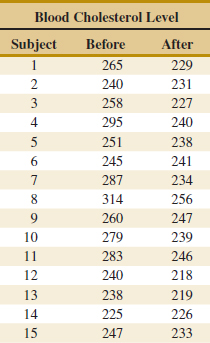
(a) Do the data support the claim that low-fat diet and aerobic exercise are of value in producing a mean reduction in blood cholesterol levels? Use α = 0.05. Find the P-value.
(b) Calculate a one-sided confidence limit that can be used to answer the question in part (a).
10-54. ![]() An article in the Journal of Aircraft (1986, Vol. 23, pp. 859–864) described a new equivalent plate analysis method formulation that is capable of modeling aircraft structures such as cranked wing boxes and that produces results similar to the more computationally intensive finite element analysis method. Natural vibration frequencies for the cranked wing box structure are calculated using both methods, and results for the first seven natural frequencies follow:
An article in the Journal of Aircraft (1986, Vol. 23, pp. 859–864) described a new equivalent plate analysis method formulation that is capable of modeling aircraft structures such as cranked wing boxes and that produces results similar to the more computationally intensive finite element analysis method. Natural vibration frequencies for the cranked wing box structure are calculated using both methods, and results for the first seven natural frequencies follow:
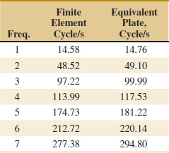
(a) Do the data suggest that the two methods provide the same mean value for natural vibration frequency? Use α = 0.05. Find the P-value.
(b) Find a 95% confidence interval on the mean difference between the two methods.
10-55. ![]() Ten individuals have participated in a diet-modification program to stimulate weight loss. Their weight both before and after participation in the program is shown in the following list.
Ten individuals have participated in a diet-modification program to stimulate weight loss. Their weight both before and after participation in the program is shown in the following list.
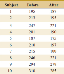
(a) Is there evidence to support the claim that this particular diet-modification program is effective in producing a mean weight reduction? Use α = 0.05.
(b) Is there evidence to support the claim that this particular diet-modification program will result in a mean weight loss of at least 10 pounds? Use α = 0.05.
(c) Suppose that, if the diet-modification program results in mean weight loss of at least 10 pounds, it is important to detect this with probability of at least 0.90. Was the use of 10 subjects an adequate sample size? If not, how many subjects should have been used?
10-56. ![]() Two different analytical tests can be used to determine the impurity level in steel alloys. Eight specimens are tested using both procedures, and the results are shown in the following tabulation.
Two different analytical tests can be used to determine the impurity level in steel alloys. Eight specimens are tested using both procedures, and the results are shown in the following tabulation.
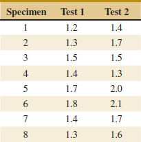
(a) Is there sufficient evidence to conclude that tests differ in the mean impurity level, using α = 0.01?
(b) Is there evidence to support the claim that test 1 generates a mean difference 0.1 units lower than test 2? Use α = 0.05.
(c) If the mean from test 1 is 0.1 less than the mean from test 2, it is important to detect this with probability at least 0.90. Was the use of eight alloys an adequate sample size? If not, how many alloys should have been used?
10-57. An article in Neurology (1998, Vol. 50, pp. 1246–1252) discussed that monozygotic twins share numerous physical, psychological, and pathological traits. The investigators measured an intelligence score of 10 pairs of twins, and the data follow:
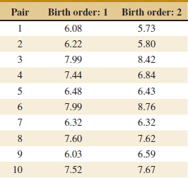
(a) Is the assumption that the difference in score is normally distributed reasonable? Show results to support your answer.
(b) Find a 95% confidence interval on the difference in mean score. Is there any evidence that mean score depends on birth order?
(c) It is important to detect a mean difference in score of one point with a probability of at least 0.90. Was the use of 10 pairs an adequate sample size? If not, how many pairs should have been used?
10-58. In Biometrics (1990, Vol. 46, pp. 673–87), the authors analyzed the circumference of five orange trees (labeled as A–E) measured on seven occasions (xi).
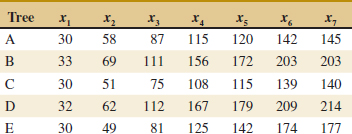
(a) Compare the mean increase in circumference in periods 1 to 2 to the mean increase in periods 2 to 3. The increase is the difference in circumference in the two periods. Are these means significantly different at α = 0.10?
(b) Is there evidence that the mean increase in period 1 to period 2 is greater than the mean increase in period 6 to period 7 at α = 0.05?
(c) Are the assumptions of the test in part (a) violated because the same data (period 2 circumference) are used to calculate both mean increases?
10-59. Use the sign test on the blood cholesterol data in Exercise 10-53. Is there evidence that diet and exercise reduce the median cholesterol level?
10-60. Repeat Exercise 10-59 using the Wilcoxon signed-rank test. State carefully what hypothesis is being tested and how it differs from the one tested in Exercise 10-59.
10-61. Neuroscientists conducted research in a Canadian prison to see whether solitary confinement affects brain wave activity [“Changes in EEG Alpha Frequency and Evoked Response Latency During Solitary Confinement,” Journal of Abnormal Psychology 1972, Vol. 7, pp. 54–59]. They randomly assigned 20 inmates to two groups, assigning half to solitary confinement and the other half to regular confinement. The data follow:
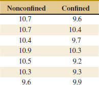

(a) Is a paired t-test appropriate for testing whether the mean alpha wave frequencies are the same in the two groups? Explain.
(b) Perform an appropriate test.
10-62. In a series of tests to study the efficacy of ginkgo biloba on memory, Solomon et al. first looked at differences in memory tests of people six weeks before and after joining the study [“Ginkgo for Memory Enhancement: A Randomized Controlled Trial,” Journal of the American Medical Association (2002, Vol. 288, pp. 835–840)]. For 99 patients receiving no medication, the average increase in category fluency (number of words generated in one minute) was 1.07 words with a standard deviation of 3.195 words. Researchers wanted to know whether the mean number of words recalled was positive.
(a) Is this a one- or two-sided test?
(b) Perform a hypothesis test to determine whether the mean increase is zero.
(c) Why can this be viewed as a paired t-test?
(d) What does the conclusion say about the importance of including placebos in such tests?
10-5 Inference on the Variances of Two Normal Distributions
We now introduce tests and confidence intervals for the two population variances shown in Fig. 10-1. We will assume that both populations are normal. Both the hypothesis-testing and confidence interval procedures are relatively sensitive to the normality assumption.
10-5.1 F DISTRIBUTION
Suppose that two independent normal populations are of interest when the population means and variances, say, μ1, ![]() , μ2, and
, μ2, and ![]() , are unknown. We wish to test hypotheses about the equality of the two variances, say, H0 :
, are unknown. We wish to test hypotheses about the equality of the two variances, say, H0 : ![]() =
= ![]() . Assume that two random samples of size n1 from population 1 and of size n2 from population 2 are available, and let
. Assume that two random samples of size n1 from population 1 and of size n2 from population 2 are available, and let ![]() and
and ![]() be the sample variances. We wish to test the hypotheses
be the sample variances. We wish to test the hypotheses
![]()
The development of a test procedure for these hypotheses requires a new probability distribution, the F distribution. The random variable F is defined to be the ratio of two independent chi-square random variables, each divided by its number of degrees of freedom. That is,
![]()
where W and Y are independent chi-square random variables with u and v degrees of freedom, respectively. We now formally state the sampling distribution of F.
Let W and Y be independent chi-square random variables with u and v degrees of freedom, respectively. Then the ratio
![]()
has the probability density function
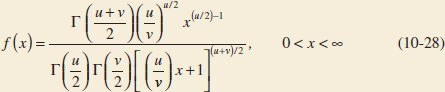
and is said to follow the F distribution with u degrees of freedom in the numerator and v degrees of freedom in the denominator. It is usually abbreviated as Fu, v.
The mean and variance of the F distribution are μ = v/(v − 2) for v > 2, and
![]()
Two F distributions are shown in Fig. 10-4. The F random variable is non-negative, and the distribution is skewed to the right. The F distribution looks very similar to the chi-square distribution; however, the two parameters u and v provide extra flexibility regarding shape.
The percentage points of the F distribution are given in Table VI of the Appendix. Let fα,u,v be the percentage point of the F distribution with numerator degrees of freedom u and denominator degrees of freedom v such that the probability that the random variable F exceeds this value is
![]()
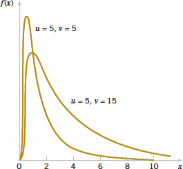
FIGURE 10-4 Probability density functions of two F distributions.
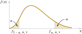
FIGURE 10-5 Upper and lower percentage points of the F distribution.
This is illustrated in Fig. 10-5. For example, if u = 5 and v = 10, we find from Table V of the Appendix that
![]()
That is, the upper 5 percentage point of F5,10 is f0.05,5,10 = 3.33.
Table VI contains only upper-tailed percentage points (for selected values of fα,u,v for α ≤ 0.25) of the F distribution. The lower-tailed percentage points f1−α,u,v can be found as follows.
Finding Lower Tail Points of the F-Distribution

For example, to find the lower-tailed percentage point f0.95,5,10, note that
![]()
10-5.2 HYPOTHESIS TESTS ON THE RATIO OF TWO VARIANCES
A hypothesis-testing procedure for the equality of two variances is based on the following result.
Distribution of the Ratio of Sample Variances from Two Normal Distributions
Let X11, X12,..., X1n1 be a random sample from a normal population with mean μ1 and variance ![]() , and let X21, X22,..., X2n2 be a random sample from a second normal population with mean μ2 and variance
, and let X21, X22,..., X2n2 be a random sample from a second normal population with mean μ2 and variance ![]() . Assume that both normal populations are independent. Let
. Assume that both normal populations are independent. Let ![]() and
and ![]() be the sample variances. Then the ratio
be the sample variances. Then the ratio
![]()
has an F distribution with n1 − 1 numerator degrees of freedom and n2 − 1 denominator degrees of freedom.
This result is based on the fact that (n1 − 1) ![]() /
/![]() is a chi-square random variable with n1 − 1 degrees of freedom, that (n2 − 1)
is a chi-square random variable with n1 − 1 degrees of freedom, that (n2 − 1) ![]() /
/![]() is a chi-square random variable with n2 − 1 degrees of freedom, and that the two normal populations are independent. Clearly, under the null hypothesis H0:
is a chi-square random variable with n2 − 1 degrees of freedom, and that the two normal populations are independent. Clearly, under the null hypothesis H0: ![]() =
= ![]() , the ratio F0 =
, the ratio F0 = ![]() /
/![]() has an Fn1 − 1, n2 − 1 distribution. This is the basis of the following test procedure.
has an Fn1 − 1, n2 − 1 distribution. This is the basis of the following test procedure.
Tests on the Ratio of Variances from Two Normal Distributions
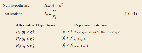
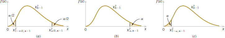
FIGURE 10-6 The F distribution for the test of H0: ![]() =
= ![]() with critical region values for (a) H1:
with critical region values for (a) H1: ![]() ≠
≠ ![]() . (b) H1:
. (b) H1: ![]() >
> ![]() . and (c) H1:
. and (c) H1: ![]() <
< ![]() .
.
The critical regions for these fixed-significance-level tests are shown in Figure 10-6. Remember that this procedure is relatively sensitive to the normality assumption.
Example 10-13 Semiconductor Etch Variability Oxide layers on semiconductor wafers are etched in a mixture of gases to achieve the proper thickness. The variability in the thickness of these oxide layers is a critical characteristic of the wafer, and low variability is desirable for subsequent processing steps. Two different mixtures of gases are being studied to determine whether one is superior in reducing the variability of the oxide thickness. Sixteen wafers are etched in each gas. The sample standard deviations of oxide thickness are s1 = 1.96 angstroms and s2 = 2.13 angstroms, respectively. Is there any evidence to indicate that either gas is preferable? Use a fixed-level test with α = 0.05.
The seven-step hypothesis-testing procedure may be applied to this problem as follows:
- Parameter of interest: The parameters of interest are the variances of oxide thickness
 and
and  . We will assume that oxide thickness is a normal random variable for both gas mixtures.
 - Null hypothesis: H0:
 =
= 
- Alternative hypothesis: H1:
 ≠
≠ 
- Test statistic: The test statistic is given by Equation 10-31:

- Reject H0 if: Because n1 = n2 = 16 and α = 0.05, we will reject H0:
 =
=  if f0 > f0.025,15,15 = 2.86 or if f0 < f0.975,15,15 = 1/f0.025,15,15 = 1/2.86 = 0.35. Refer to Figure 10-6(a).
 - Computations: Because
 = (1.96)2 = 3.84 and
  = (2.13)2 = 4.54, the test statistic is
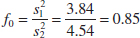
- Conclusion: Because f0.975,15,15 = 0.35 < 0.85 < f0.025,15,15 = 2.86, we cannot reject the null hypothesis H0:
 =
=  at the 0.05 level of significance.
Practical Interpretation: There is no strong evidence to indicate that either gas results in a smaller variance of oxide thickness.
P-Values for the F-Test
The P-value approach can also be used with F-tests. To show how to do this, consider the upper-tailed one-tailed test. The P-value is the area (probability) under the F distribution with n1 − 1 and n2 − 1 degrees of freedom that lies beyond the computed value of the test statistic f0. Appendix A Table IV can be used to obtain upper and lower bounds on the P-value. For example, consider an F-test with 9 numerator and 14 denominator degrees of freedom for which f0 = 3.05. From Appendix A Table IV, we find that f0.05,9,14 = 2.65 and f0.025,9,14 = 3.21, so because f0 = 3.05 lies between these two values, the P-value is between 0.05 and 0.025; that is, 0.025 < P < 0.05. The P-value for a lower-tailed test would be found similarly, although Appendix A Table IV contains only upper-tailed points of the F distribution, Equation 10-30 would have to be used to find the necessary lower-tail points. For a two-tailed test, the bounds obtained from a one-tailed test would be doubled to obtain the P-value.
Finding the P-Value for Example 10-13
To illustrate calculating bounds on the P-value for a two-tailed F-test, reconsider Example 10-13. The computed value of the test statistic in this example is f0 = 0.85. This value falls in the lower tail of the F15,15 distribution. The lower-tailed point that has 0.25 probability to the left of it is f0.75,15,15 = 1/f0.25,15,15 = 1/1.43 = 0.70, and because 0.70 < 0.85, the probability that lies to the left of 0.85 exceeds 0.25. Therefore, we would conclude that the P-value for f0 = 0.85 is greater than 2(0.25) = 0.5, so there is insufficient evidence to reject the null hypothesis. This is consistent with the original conclusions from Example 10-13. The actual P-value is 0.7570. This value was obtained from a calculator from which we found that P(F15,15 ≤ 0.85) = 0.3785 and 2(0.3785) = 0.7570. Computer software can also be used to calculate the required probabilities.
Some computer packages will perform the F-test on the equality of two variances of independent normal distributions. The output from the computer package follows.
Test for Equal Variances
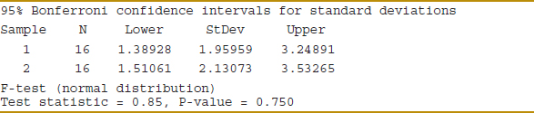
Computer software also gives confidence intervals on the individual variances. These are the confidence intervals originally given in Equation 8-19 except that a Bonferroni “adjustment” has been applied to make the confidence level for both intervals simultaneously equal to at least 95%. This consists of using α/2 = 0.05/2 = 0.025 to construct the individual intervals. That is, each individual confidence interval is a 97.5% CI. In Section 10-5.4, we will show how to construct a CI on the ratio of the two variances.
10-5.3 TYPE II ERROR AND CHOICE OF SAMPLE SIZE
Appendix Charts VIIo, VIIp, VIIq, and VIIr provide operating characteristic curves for the F-test given in Section 10-5.1 for α = 0.05 and α = 0.01, assuming that n1 = n2 = n. Charts VIIo and VIIp are used with the two-sided alternate hypothesis. They plot β against the abscissa parameter
![]()
for various n1 = n2 = n. Charts VIIq and VIIr are used for the one-sided alternative hypotheses.
Example 10-14 Semiconductor Etch Variability Sample Size For the semiconductor wafer oxide etching problem in Example 10-13, suppose that one gas resulted in a standard deviation of oxide thickness that is half the standard deviation of oxide thickness of the other gas. If we wish to detect such a situation with probability at least 0.80, is the sample size n1 = n2 = 20 adequate?
Note that if one standard deviation is half the other,
![]()
By referring to Appendix Chart VIIo with n1 = n2 = 20 and λ = 2, we find that β ![]() 0.20. Therefore, if β
0.20. Therefore, if β ![]() 0.20, the power of the test (which is the probability that the difference in standard deviations will be detected by the test) is 0.80, and we conclude that the sample sizes n1 = n2 = 20 are adequate.
0.20, the power of the test (which is the probability that the difference in standard deviations will be detected by the test) is 0.80, and we conclude that the sample sizes n1 = n2 = 20 are adequate.
10-5.4 CONFIDENCE INTERVAL ON THE RATIO OF TWO VARIANCES
To find the confidence interval on ![]() /
/![]() , recall that the sampling distribution of
, recall that the sampling distribution of
![]()
is an F with n2 − 1 and n1 − 1 degrees of freedom. Therefore, P(f1−α/2,n2−1,n1−1 ≤ F ≤ fα/2,n2−1,n1−1) = 1 − α. Substitution for F and manipulation of the inequalities will lead to the 100(1 − α)% confidence interval for ![]() /
/![]() .
.
Confidence Interval on the Ratio of Variances from Two Normal Distributions
If ![]() and
and ![]() are the sample variances of random samples of sizes n1 and n2, respectively, from two independent normal populations with unknown variances
are the sample variances of random samples of sizes n1 and n2, respectively, from two independent normal populations with unknown variances ![]() and
and ![]() , then a 100(1 − α)% confidence interval on the ratio
, then a 100(1 − α)% confidence interval on the ratio ![]() /
/![]() is
is
![]()
where fα/2,n2−1,n1−1 and f1−α/2,n2−1,n1−1 are the upper and lower α/2 percentage points of the F distribution with n2 − 1 numerator and n1 − 1 denominator degrees of freedom, respectively. A confidence interval on the ratio of the standard deviations can be obtained by taking square roots in Equation 10-33.
Just as in the hypothesis testing procedure, this CI is relatively sensitive to the normality assumption.
Example 10-15 Surface Finish for Titanium Alloy A company manufactures impellers for use in jet-turbine engines. One of the operations involves grinding a particular surface finish on a titanium alloy component. Two different grinding processes can be used, and both processes can produce parts at identical mean surface roughness. The manufacturing engineer would like to select the process having the least variability in surface roughness. A random sample of n1 = 11 parts from the first process results in a sample standard deviation s1 = 5.1 microinches, and a random sample of n2 = 16 parts from the second process results in a sample standard deviation of s2 = 4.7 microinches. We will find a 90% confidence interval on the ratio of the two standard deviations, σ1/σ2.
Assuming that the two processes are independent and that surface roughness is normally distributed, we can use Equation 10-33 as follows:
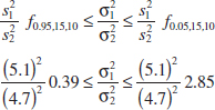
or upon completing the implied calculations and taking square roots,
![]()
Notice that we have used Equation 10-30 to find f0.95,15,10 = 1/f0.05,10,15 = 1/2.54 = 0.39.
Practical Interpretation: Because this confidence interval includes unity, we cannot claim that the standard deviations of surface roughness for the two processes are different at the 90% level of confidence.
Exercises FOR SECTION 10-5
![]() Problem available in WileyPLUS at instructor's discretion.
Problem available in WileyPLUS at instructor's discretion.
![]() Go Tutorial Tutoring problem available in WileyPLUS at instructor's discretion.
Go Tutorial Tutoring problem available in WileyPLUS at instructor's discretion.
10-63. For an F distribution, find the following:
(a) f0.25,5,10
(b) f0.10,24,9
(c) f0.05,8,15
(d) f0.75,5,10
(e) f0.90,24,9
(f) f0.95,8,15
10-64. For an F distribution, find the following:
(a) f0.25,7,15
(b) f0.10,10,12
(c) f0.01,20,10
(d) f0.75,7,15
(e) f0.90,10,12
(f) f0.99,20,10
10-65. Consider the hypothesis test H0: ![]() =
= ![]() against H1:
against H1: ![]() <
< ![]() respectively. Suppose that the sample sizes are n1 = 5 and n2 = 10, and that
respectively. Suppose that the sample sizes are n1 = 5 and n2 = 10, and that ![]() = 23.2 and
= 23.2 and ![]() = 28.8. Use α = 0.05. Test the hypothesis and explain how the test could be conducted with a confidence interval on σ1/σ2.
= 28.8. Use α = 0.05. Test the hypothesis and explain how the test could be conducted with a confidence interval on σ1/σ2.
10-66. Consider the hypothesis test H0: ![]() =
= ![]() against H1:
against H1: ![]() >
> ![]() . Suppose that the sample sizes are n1 = 20 and n2 = 8, and that
. Suppose that the sample sizes are n1 = 20 and n2 = 8, and that ![]() = 4.5 and
= 4.5 and ![]() = 2.3. Use α = 0.01. Test the hypothesis and explain how the test could be conducted with a confidence interval on σ1/σ2.
= 2.3. Use α = 0.01. Test the hypothesis and explain how the test could be conducted with a confidence interval on σ1/σ2.
10-67. Consider the hypothesis test H0: ![]() =
= ![]() against H1:
against H1: ![]() ≠
≠ ![]() . Suppose that the sample sizes are n1 = 15 and n2 = 15, and the sample variances are
. Suppose that the sample sizes are n1 = 15 and n2 = 15, and the sample variances are ![]() = 2.3 and
= 2.3 and ![]() = 1.9. Use α = 0.05.
= 1.9. Use α = 0.05.
(a) Test the hypothesis and explain how the test could be conducted with a confidence interval on σ1/σ2.
(b) What is the power of the test in part (a) if σ1 is twice as large as σ2?
(c) Assuming equal sample sizes, what sample size should be used to obtain β = 0.05 if the σ2 is half of σ1?
10-68. ![]() Two chemical companies can supply a raw material. The concentration of a particular element in this material is important. The mean concentration for both suppliers is the same, but you suspect that the variability in concentration may differ for the two companies. The standard deviation of concentration in a random sample of n1 = 10 batches produced by company 1 is s1 = 4.7 grams per liter, and for company 2, a random sample of n2 = 16 batches yields s2 = 5.8 grams per liter. Is there sufficient evidence to conclude that the two population variances differ? Use α = 0.05.
Two chemical companies can supply a raw material. The concentration of a particular element in this material is important. The mean concentration for both suppliers is the same, but you suspect that the variability in concentration may differ for the two companies. The standard deviation of concentration in a random sample of n1 = 10 batches produced by company 1 is s1 = 4.7 grams per liter, and for company 2, a random sample of n2 = 16 batches yields s2 = 5.8 grams per liter. Is there sufficient evidence to conclude that the two population variances differ? Use α = 0.05.
10-69. ![]() A study was performed to determine whether men and women differ in repeatability in assembling components on printed circuit boards. Random samples of 25 men and 21 women were selected, and each subject assembled the units. The two sample standard deviations of assembly time were smen = 0.98 minutes and swomen = 1.02 minutes.
A study was performed to determine whether men and women differ in repeatability in assembling components on printed circuit boards. Random samples of 25 men and 21 women were selected, and each subject assembled the units. The two sample standard deviations of assembly time were smen = 0.98 minutes and swomen = 1.02 minutes.
(a) Is there evidence to support the claim that men and women differ in repeatability for this assembly task? Use α = 0.02 and state any necessary assumptions about the underlying distribution of the data.
(b) Find a 98% confidence interval on the ratio of the two variances. Provide an interpretation of the interval.
10-70. Consider the foam data in Exercise 10-20. Construct the following:
(a) ![]() Go Tutorial A 90% two-sided confidence interval on
Go Tutorial A 90% two-sided confidence interval on ![]() /
/![]() .
.
(b) ![]() A 95% two-sided confidence interval on
A 95% two-sided confidence interval on ![]() /
/![]() . Comment on the comparison of the width of this interval with the width of the interval in part (a).
. Comment on the comparison of the width of this interval with the width of the interval in part (a).
(c) ![]() Go Tutorial A 90% lower-confidence bound on σ1/σ2.
Go Tutorial A 90% lower-confidence bound on σ1/σ2.
10-71. Consider the diameter data in Exercise 10-19. Construct the following:
(a) A 90% two-sided confidence interval on σ1/σ2.
(b) A 95% two-sided confidence interval on σ1/σ2. Comment on the comparison of the width of this interval with the width of the interval in part (a).
(c) A 90% lower-confidence bound on σ1/σ2.
10-72. ![]() Consider the gear impact strength data in Exercise 10-24. Is there sufficient evidence to conclude that the variance of impact strength is different for the two suppliers? Use α = 0.05.
Consider the gear impact strength data in Exercise 10-24. Is there sufficient evidence to conclude that the variance of impact strength is different for the two suppliers? Use α = 0.05.
10-73. Consider the melting-point data in Exercise 10-25. Do the sample data support a claim that both alloys have the same variance of melting point? Use α = 0.05 in reaching your conclusion.
10-74. Exercise 10-28 presented measurements of plastic coating thickness at two different application temperatures. Test H0: ![]() =
= ![]() against H1:
against H1: ![]() ≠
≠ ![]() using α = 0.01.
using α = 0.01.
10-75. ![]() Reconsider the overall distance data for golf balls in Exercise 10-33. Is there evidence to support the claim that the standard deviation of overall distance is the same for both brands of balls (use α = 0.05)? Explain how this question can be answered with a 95% confidence interval on σ1/σ2.
Reconsider the overall distance data for golf balls in Exercise 10-33. Is there evidence to support the claim that the standard deviation of overall distance is the same for both brands of balls (use α = 0.05)? Explain how this question can be answered with a 95% confidence interval on σ1/σ2.
10-76. Reconsider the coefficient of restitution data in Exercise 10-34. Do the data suggest that the standard deviation is the same for both brands of drivers (use α = 0.05)? Explain how to answer this question with a confidence interval on σ1/σ2.
10-77. Consider the weight of paper data from Technometrics in Exercise 10-32. Is there evidence that the variance of the weight measurement differs for the sheets of paper? Use α = 0.05. Explain how this test can be conducted with a confidence interval.
10-78. Consider the film speed data in Exercise 10-26.
(a) Test H0: ![]() =
= ![]() versus H1:
versus H1: ![]() ≠
≠ ![]() using α = 0.02.
using α = 0.02.
(b) Suppose that one population standard deviation is 50% larger than the other. Is the sample size n1 = n2 = 8 adequate to detect this difference with high probability? Use α = 0.01 in answering this question.
10-79. Consider the etch rate data in Exercise 10-23.
(a) Test the hypothesis H0: ![]() =
= ![]() against H1:
against H1: ![]() ≠
≠ ![]() using α = 0.05, and draw conclusions.
using α = 0.05, and draw conclusions.
(a) Suppose that if one population variance is twice as large as the other, you want to detect this with probability at least 0.90 (using α = 0.05). Are the sample sizes n1 = n2 = 10 adequate?
10-80. Consider the swimming data in Exercise 10-37. Is there evidence to suggest that the standard deviations of the heats differ for slower swimmers in heat five and the faster swimmers in heat seven? What about the standard deviations of the two sets of elite swimmers in heats six and seven? Use α = 0.05.
10-81. Is there evidence to suggest that the standard deviations of the algae concentrations in the two types of rivers (flow rates) in Exercise 10-36 differ? Use α = 0.05.
10-6 Inference on Two Population Proportions
We now consider the case with two binomial parameters of interest, say, p1 and p2, and we wish to draw inferences about these proportions. We will present large-sample hypothesis testing and confidence interval procedures based on the normal approximation to the binomial.
10-6.1 LARGE-SAMPLE TESTS ON THE DIFFERENCE IN POPULATION PROPORTIONS
Suppose that two independent random samples of sizes n1 and n2 are taken from two populations, and let X1 and X2 represent the number of observations that belong to the class of interest in samples 1 and 2, respectively. Furthermore, suppose that the normal approximation to the binomial is applied to each population, so the estimators of the population proportions P1 = X1/n1 and P2 = X2/n2 have approximate normal distributions. We are interested in testing the hypotheses
![]()
The statistic
Test Statistic for the Difference of Two Population Proportions
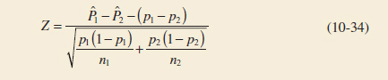
is distributed approximately as standard normal and is the basis of a test for H0: p1 = p2. Specifically, if the null hypothesis H0 : p1 = p2 is true, by using the fact that p1 = p2 = p, the random variable
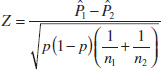
is distributed approximately N(0,1). A pooled estimator of the common parameter p is
![]()
The test statistic for H0: p1 = p2 is then
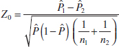
This leads to the test procedures described as follows.
Approximate Tests on the Difference of Two Population Proportions
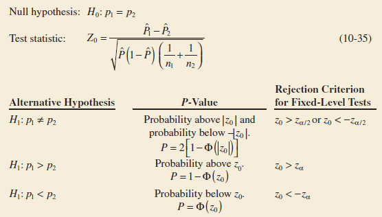
Example 10-16 St. John's Wort Extracts of St. John's Wort are widely used to treat depression. An article in the April 18, 2001, issue of the Journal of the American Medical Association (“Effectiveness of St. John's Wort on Major Depression: A Randomized Controlled Trial”) compared the efficacy of a standard extract of St. John's Wort with a placebo in 200 outpatients diagnosed with major depression. Patients were randomly assigned to two groups; one group received the St. John's Wort, and the other received the placebo. After eight weeks, 19 of the placebo-treated patients showed improvement, and 27 of those treated with St. John's Wort improved. Is there any reason to believe that St. John's Wort is effective in treating major depression? Use α = 0.05.
The seven-step hypothesis testing procedure leads to the following results:
- Parameter of interest: The parameters of interest are p1 and p2, the proportion of patients who improve following treatment with St. John's Wort (p1) or the placebo (p2).
- Null hypothesis: H0 : p1 = p2
- Alternative hypothesis: H1 : p1 ≠ p2
- Test statistic: The test statistic is
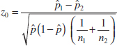
where
 1 = 27/100 = 0.27,2 = 19/100 = 0.19, n1 = n2 = 100, and
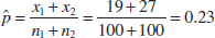
- Reject H0 if: Reject H0 : p1 = p2 if the P-value is less than 0.05.
- Computation: The value of the test statistic is
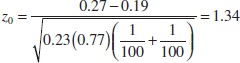
- Conclusion: Because z0 = 1.34, the P-value is P = 2[1 − Φ(1.34)] = 0.18, so, we cannot reject the null hypothesis.
Practical Interpretation: There is insufficient evidence to support the claim that St. John's Wort is effective in treating major depression.
The following display shows a typical computer output for the two-sample hypothesis test and CI procedure for proportions. Notice that the 95% CI on p1 − p2 includes zero. The equation for constructing the CI will be given in Section 10-6.3.
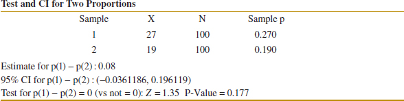
10-6.2 TYPE II ERROR AND CHOICE OF SAMPLE SIZE
The computation of the β-error for the large-sample test of H0: p1 = p2 is somewhat more involved than in the single-sample case. The problem is that the denominator of the test statistic Z0 is an estimate of the standard deviation of ![]() 1 −
1 − ![]() 2 under the assumption that p1 = p2 = p. When H0 : p1 = p2 is false, the standard deviation of
2 under the assumption that p1 = p2 = p. When H0 : p1 = p2 is false, the standard deviation of ![]() 1 −
1 − ![]() 2 is
2 is
![]()
Approximate Type II Error for a Two-Sided Test on the Difference of Two Population Proportions
If the alternative hypothesis is two sided, the β-error is
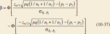
![]()
and ![]() is given by Equation 10-36.
is given by Equation 10-36.
Approximate Type II Error for a One-Sided Test on the Difference of Two Population Proportions
If the alternative hypothesis is H1 : p1 > p2,
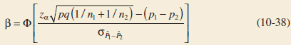
and if the alternative hypothesis is H1 : p1 < p2,
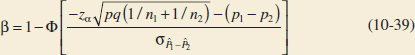
For a specified pair of values p1 and p2, we can find the sample sizes n1 = n2 = n required to give the test of size α that has specified type II error β.
Approximate Sample Size for a Two-Sided Test on the Difference in Population Proportions
For the two-sided alternative, the common sample size is
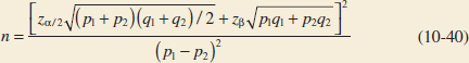
where q1 = 1 − p1 and q2 = 1 − p2.
For a one-sided alternative, replace zα/2 in Equation 10-40 by zα.
10-6.3 CONFIDENCE INTERVAL ON THE DIFFERENCE IN POPULATION PROPORTIONS
The traditional confidence interval for p1 − p2 can be found directly because we know that
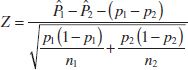
is approximately a standard normal random variable. Thus P(−zα/2 ≤ Z ≤ zα/2) ![]() 1 − α, so we can substitute for Z in this last expression and use an approach similar to the one employed previously to find an approximate 100(1 − α)% two-sided confidence interval for p1 − p2.
1 − α, so we can substitute for Z in this last expression and use an approach similar to the one employed previously to find an approximate 100(1 − α)% two-sided confidence interval for p1 − p2.
If ![]() 1 and
1 and ![]() 2 are the sample proportions of observations in two independent random samples of sizes n1 and n2 that belong to a class of interest, an approximate two-sided 100(1 − α)% confidence interval on the difference in the true proportions p1 − p2 is
2 are the sample proportions of observations in two independent random samples of sizes n1 and n2 that belong to a class of interest, an approximate two-sided 100(1 − α)% confidence interval on the difference in the true proportions p1 − p2 is
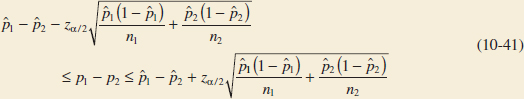
where Zα/2 is the upper α/2 percentage point of the standard normal distribution.
Example 10-17 Defective Bearings Consider the process of manufacturing crankshaft bearings described in Example 8-8. Suppose that a modification is made in the surface finishing process and that, subsequently, a second random sample of 85 bearings is obtained. The number of defective bearings in this second sample is 8. Therefore, because n1 = 85, ![]() 1 = 10/85 = 0.1176, n2 = 85, and
1 = 10/85 = 0.1176, n2 = 85, and ![]() 2 = 8/85 = 0.0941, we can obtain an approximate 95% confidence interval on the difference in the proportion of defective bearings produced under the two processes from Equation 10-41 as follows:
2 = 8/85 = 0.0941, we can obtain an approximate 95% confidence interval on the difference in the proportion of defective bearings produced under the two processes from Equation 10-41 as follows:
![]()
or
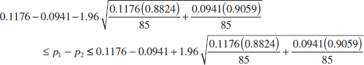
This simplifies to
![]()
Practical Interpretation: This confidence interval includes zero, so, based on the sample data, it seems unlikely that the changes made in the surface finish process have reduced the proportion of defective crankshaft bearings being produced.
The CI in Equation 10-41 is the traditional one usually given for a difference in two binomial proportions. However, the actual confidence level for this interval can deviate substantially from the nominal or advertised value. So when we want a 95% CI (for example) and use z0.025 = 1.96 in Equation 10-41, the actual confidence level that we experience may differ from 95%. This situation can be improved by a very simple adjustment to the procedure: Add one success and one failure to the data from each sample and then calculate
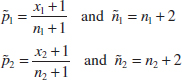
Then replace ![]() 1,
1, ![]() 2, n1 and n2 by
2, n1 and n2 by ![]() 1,
1, ![]() 2,
2, ![]() 1 and
1 and ![]() 2 in Equation 10-41.
2 in Equation 10-41.
To illustrate how this works, reconsider the crankshaft bearing data from Example 10-17. Using the preceding procedure, we find that
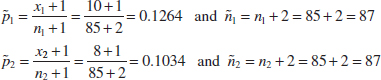
If we now replace ![]() 1,
1, ![]() 2, n1 and n2 by
2, n1 and n2 by ![]() 1,
1, ![]() 2,
2, ![]() 1 and
1 and ![]() 2 in Equation 10-41, we find that the new improved CI is −0.0730 ≤ p1 − p2 ≤ 0.1190, which is similar to the traditional CI found in Example 10-17. The length of the traditional interval is 0.1840, and the length of the new and improved interval is 0.1920. The slightly longer interval is likely a reflection of the fact that the coverage of the improved interval is closer to the advertised level of 95%. However, because this CI also includes zero, the conclusions would be the same regardless of which CI is used.
2 in Equation 10-41, we find that the new improved CI is −0.0730 ≤ p1 − p2 ≤ 0.1190, which is similar to the traditional CI found in Example 10-17. The length of the traditional interval is 0.1840, and the length of the new and improved interval is 0.1920. The slightly longer interval is likely a reflection of the fact that the coverage of the improved interval is closer to the advertised level of 95%. However, because this CI also includes zero, the conclusions would be the same regardless of which CI is used.
Exercises FOR SECTION 10-6
![]() Problem available in WileyPLUS at instructor's discretion.
Problem available in WileyPLUS at instructor's discretion.
![]() Go Tutorial Tutoring problem available in WileyPLUS at instructor's discretion.
Go Tutorial Tutoring problem available in WileyPLUS at instructor's discretion.
10-82. Consider the following computer output.
Test and Cl for Two Proportions
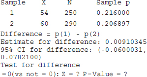
(a) Is this a one-sided or a two-sided test?
(b) Fill in the missing values.
(c) Can the null hypothesis be rejected?
(d) Construct an approximate 90% CI for the difference in the two proportions.
10-83. Consider the following computer output.
Test and CI for Two Proportions
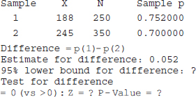
(a) Is this one-sided or a two-sided test?
(b) Fill in the missing values.
(c) ![]() Go Tutorial Can the null hypothesis be rejected if = 0.10? What if = 0.05?
Go Tutorial Can the null hypothesis be rejected if = 0.10? What if = 0.05?
10-84. ![]() An article in Knee Surgery, Sports Traumatology, Arthroscopy (2005, Vol. 13, pp. 273–279) considered arthroscopic meniscal repair with an absorbable screw. Results showed that for tears greater than 25 millimeters, 14 of 18 (78%) repairs were successful, but for shorter tears, 22 of 30 (73%) repairs were successful.
An article in Knee Surgery, Sports Traumatology, Arthroscopy (2005, Vol. 13, pp. 273–279) considered arthroscopic meniscal repair with an absorbable screw. Results showed that for tears greater than 25 millimeters, 14 of 18 (78%) repairs were successful, but for shorter tears, 22 of 30 (73%) repairs were successful.
(a) Is there evidence that the success rate is greater for longer tears? Use α = 0.05. What is the P-value?
(b) Calculate a one-sided 95% confidence bound on the difference in proportions that can be used to answer the question in part (a).
10-85. ![]() In the 2004 presidential election, exit polls from the critical state of Ohio provided the following results: For respondents with college degrees, 53% voted for Bush and 46% voted for Kerry. There were 2020 respondents.
In the 2004 presidential election, exit polls from the critical state of Ohio provided the following results: For respondents with college degrees, 53% voted for Bush and 46% voted for Kerry. There were 2020 respondents.
(a) Is there a significant difference in these proportions? Use α = 0.05. What is the P-value?
(b) Calculate a 95% confidence interval for the difference in the two proportions and comment on the use of this interval to answer the question in part (a).
10-86. Two different types of injection-molding machines are used to form plastic parts. A part is considered defective if it has excessive shrinkage or is discolored. Two random samples, each of size 300, are selected, and 15 defective parts are found in the sample from machine 1, and 8 defective parts are found in the sample from machine 2.
(a) Is it reasonable to conclude that both machines produce the same fraction of defective parts, using α = 0.05? Find the P-value for this test.
(b) Construct a 95% confidence interval on the difference in the two fractions defective.
(c) Suppose that p1 = 0.05 and p2 = 0.01. With the sample sizes given here, what is the power of the test for this two-sided alternate?
(d) Suppose that p1 = 0.05 and p2 = 0.01. Determine the sample size needed to detect this difference with a probability of at least 0.9.
(e) Suppose that p1 = 0.05 and p2 = 0.02. With the sample sizes given here, what is the power of the test for this two-sided alternate?
(f) Suppose that p1 = 0.05 and p2 = 0.02. Determine the sample size needed to detect this difference with a probability of at least 0.9.
10-87. Two different types of polishing solutions are being evaluated for possible use in a tumble-polish operation for manufacturing interocular lenses used in the human eye following cataract surgery. Three hundred lenses were tumble polished using the first polishing solution, and of this number, 253 had no polishing-induced defects. Another 300 lenses were tumble-polished using the second polishing solution, and 196 lenses were satisfactory upon completion.
(a) Is there any reason to believe that the two polishing solutions differ? Use α = 0.01. What is the P-value for this test?
(b) Discuss how this question could be answered with a confidence interval on p1 − p2.
10-88. A random sample of 500 adult residents of Maricopa County indicated that 385 were in favor of increasing the highway speed limit to 75 mph, and another sample of 400 adult residents of Pima County indicated that 267 were in favor of the increased speed limit.
(a) Do these data indicate that there is a difference in the support for increasing the speed limit for the residents of the two counties? Use α = 0.05. What is the P-value for this test?
(b) Construct a 95% confidence interval on the difference in the two proportions. Provide a practical interpretation of this interval.
10-89. Air pollution has been linked to lower birthweight in babies. In a study reported in the Journal of the American Medical Association, researchers examined the proportion of low-weight babies born to mothers exposed to heavy doses of soot and ash during the World Trade Center attack of September 11, 2001. Of the 182 babies born to these mothers, 15 were classified as having low weight. Of 2300 babies born in the same time period in New York in another hospital, 92 were classified as having low weight. Is there evidence to suggest that the exposed mothers had a higher incidence of low-weight babies?
10-90. The New England Journal of Medicine reported an experiment to judge the efficacy of surgery on men diagnosed with prostate cancer. The randomly assigned half of 695 (347) men in the study had surgery, and 18 of them eventually died of prostate cancer compared with 31 of the 348 who did not have surgery. Is there any evidence to suggest that the surgery lowered the proportion of those who died of prostate cancer?
10-91. Rework the election data reported in Exercise 10-85 using the alternate CI procedure described in this section. Compare the lengths of the CI from Exercise 10-85 with this one. Discuss the possible causes of any differences that you observe.
10-92. Consider the highway speed limit data introduced in Exercise 10-88. Find a 99% CI on the difference in the two proportions using the alternate CI procedure described in this section. Compare the lengths of the CI from Exercise 10-88 with these in this one. Discuss the possible causes of any differences that you observe.
10-7 Summary Table and Road Map for Inference Procedures for Two Samples
The table in the end pages of the book summarizes all of the two-sample parametric inference procedures given in this chapter. The table contains the null hypothesis statements, the test statistics, the criteria for rejection of the various alternative hypotheses, and the formulas for constructing the 100(1 − α)% confidence intervals.
The road map to select the appropriate parametric confidence interval formula or whypothesis test method for one-sample problems was presented in Table 8-1. In Table 10-5, we extend the road map to two-sample problems. The primary comments stated previously also apply here (except that we usually apply conclusions to a function of the parameters from each sample, such as the difference in means):
- Determine the function of the parameters (and the distribution of the data) that is to be bounded by the confidence interval or tested by the hypothesis.
- Check whether other parameters are known or need to be estimated (and whether any assumptions are made).
![]() TABLE • 10-5 Roadmap to Construct Confidence Intervals and Hypothesis Tests, Two-Sample Case
TABLE • 10-5 Roadmap to Construct Confidence Intervals and Hypothesis Tests, Two-Sample Case
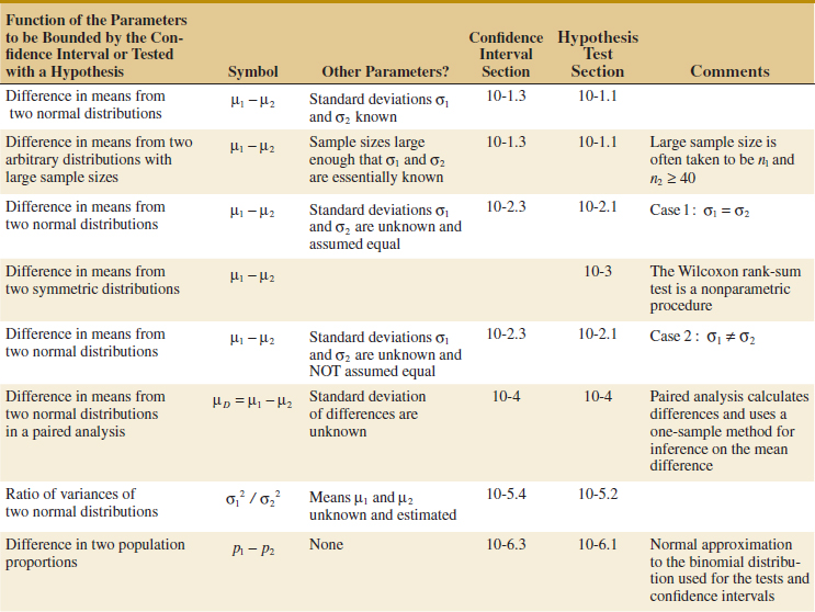
Supplemental Exercises
![]() Problem available in WileyPLUS at instructor's discretion.
Problem available in WileyPLUS at instructor's discretion.
![]() Go Tutorial Tutoring problem available in WileyPLUS at instructor's discretion.
Go Tutorial Tutoring problem available in WileyPLUS at instructor's discretion.
10-93. ![]() Consider the following computer output.
Consider the following computer output.
Two-Sample T-Test and Cl
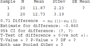
(a) Fill in the missing values. You may use bounds for the P-value.
(b) Is this a two-sided test or a one-sided test?
(c) What are your conclusions if α = 0.05? What if α = 0.10?
10-94. Consider the following computer output.
Two-Sample T-Test CI
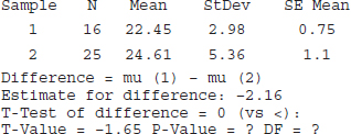
(a) Is this a one-sided or a two-sided test?
(b) Fill in the missing values. You may use bounds for the P-value.
(c) What are your conclusions if α = 0.05? What if α = 0.10?
(d) Find a 95% upper-confidence bound on the difference in the two means.
10-95. An article in the Journal of Materials Engineering [1989, Vol. 11(4), pp. 275–282] reported the results of an experiment to determine failure mechanisms for plasmasprayed thermal barrier coatings. The failure stress for one particular coating (NiCrAlZr) under two different test conditions is as follows:
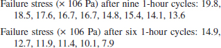
(a) What assumptions are needed to construct confidence intervals for the difference in mean failure stress under the two different test conditions? Use normal probability plots of the data to check these assumptions.
(b) Find a 99% confidence interval on the difference in mean failure stress under the two different test conditions.
(c) Using the confidence interval constructed in part (b), does the evidence support the claim that the first test conditions yield higher results, on the average, than the second? Explain your answer.
(d) Construct a 95% confidence interval on the ratio of the variances, ![]() /
/![]() , of failure stress under the two different test conditions.
, of failure stress under the two different test conditions.
(e) Use your answer in part (d) to determine whether there is a significant difference in the variances of the two different test conditions. Explain your answer.
10-96. A procurement specialist has purchased 25 resistors from vendor 1 and 35 resistors from vendor 2. Each resistor's resistance is measured with the following results (ohm):
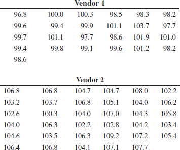
(a) What distributional assumption is needed to test the claim that the variance of resistance of the product from vendor 1 is not significantly different from the variance of resistance of the product from vendor 2? Perform a graphical procedure to check this assumption.
(b) Perform an appropriate statistical hypothesis-testing procedure to determine whether the procurement specialist can claim that the variance of resistance of the product from vendor 1 is significantly different from the variance of resistance of the product from vendor 2.
10-97. A liquid dietary product implies in its advertising that using the product for one month results in an average weight loss of at least 3 pounds. Eight subjects use the product for one month, and the resulting weight loss data follow. Use hypothesis-testing procedures to answer the following questions.
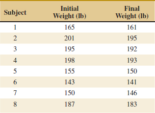
(a) Do the data support the claim of the dietary product's producer with the probability of a type I error set to 0.05?
(b) Do the data support the claim of the dietary product's producer with the probability of a type I error set to 0.01?
(c) In an effort to improve sales, the producer is considering changing its claim from “at least 3 pounds” to “at least 5 pounds.” Repeat parts (a) and (b) to test this new claim.
10-98. ![]() The breaking strength of yarn supplied by two manufacturers is being investigated. You know from experience with the manufacturers' processes that σ1 = 5 psi and σ2 = 4 psi. A random sample of 20 test specimens from each manufacturer results in
The breaking strength of yarn supplied by two manufacturers is being investigated. You know from experience with the manufacturers' processes that σ1 = 5 psi and σ2 = 4 psi. A random sample of 20 test specimens from each manufacturer results in ![]() 1 = 88 psi and
1 = 88 psi and ![]() 2 = 91 psi, respectively.
2 = 91 psi, respectively.
(a) Using a 90% confidence interval on the difference in mean breaking strength, comment on whether or not there is evidence to support the claim that manufacturer 2 produces yarn with higher mean breaking strength.
(b) Using a 98% confidence interval on the difference in mean breaking strength, comment on whether or not there is evidence to support the claim that manufacturer 2 produces yarn with higher mean breaking strength.
(c) Comment on why the results from parts (a) and (b) are different or the same. Which would you choose to make your decision and why?
10-99. The Salk polio vaccine experiment in 1954 focused on the effectiveness of the vaccine in combating paralytic polio. Because it was believed that without a control group of children, there would be no sound basis for evaluating the efficacy of the Salk vaccine, the vaccine was administered to one group, and a placebo (visually identical to the vaccine but known to have no effect) was administered to a second group. For ethical reasons and because it was suspected that knowledge of vaccine administration would affect subsequent diagnoses, the experiment was conducted in a double-blind fashion. That is, neither the subjects nor the administrators knew who received the vaccine and who received the placebo. The actual data for this experiment are as follows:
Placebo group: n = 201,299: 110 cases of polio observed
Vaccine group: n = 200,745: 33 cases of polio observed
(a) Use a hypothesis-testing procedure to determine whether the proportion of children in the two groups who contracted paralytic polio is statistically different. Use a probability of a type I error equal to 0.05.
(b) Repeat part (a) using a probability of a type I error equal to 0.01.
(c) Compare your conclusions from parts (a) and (b) and explain why they are the same or different.
10-100. Consider Supplemental Exercise 10-98. Suppose that prior to collecting the data, you decide that you want the error in estimating μ1 − μ2 by ![]() 1 −
1 − ![]() 2 to be less than 1.5 psi. Specify the sample size for the following percentage confidence:
2 to be less than 1.5 psi. Specify the sample size for the following percentage confidence:
(a) 90%
(b) 98%
(c) Comment on the effect of increasing the percentage confidence on the sample size needed.
(d) Repeat parts (a)–(c) with an error of less than 0.75 psi instead of 1.5 psi.
(e) Comment on the effect of decreasing the error on the sample size needed.
10-101. ![]() A random sample of 1500 residential telephones in Phoenix in 1990 indicated that 387 of the numbers were unlisted. A random sample of 1200 telephones in the same year in Scottsdale indicated that 310 were unlisted.
A random sample of 1500 residential telephones in Phoenix in 1990 indicated that 387 of the numbers were unlisted. A random sample of 1200 telephones in the same year in Scottsdale indicated that 310 were unlisted.
(a) Find a 95% confidence interval on the difference in the two proportions and use this confidence interval to determine 2010 whether there is a statistically significant difference in proportions of unlisted numbers between the two cities.
(b) Find a 90% confidence interval on the difference in the two proportions and use this confidence interval to determine if there is a statistically significant difference in proportions of unlisted numbers for the two cities.
(c) Suppose that all the numbers in the problem description were doubled. That is, 774 residents of 3000 sampled in Phoenix and 620 residents of 2400 in Scottsdale had unlisted phone numbers. Repeat parts (a) and (b) and comment on the effect of increasing the sample size without changing the proportions on your results.
10-102. ![]() Go Tutorial In a random sample of 200 Phoenix residents who drive a domestic car, 165 reported wearing their seat belt regularly, and another sample of 250 Phoenix residents who drive a foreign car revealed 198 who regularly wore their seat belt.
Go Tutorial In a random sample of 200 Phoenix residents who drive a domestic car, 165 reported wearing their seat belt regularly, and another sample of 250 Phoenix residents who drive a foreign car revealed 198 who regularly wore their seat belt.
(a) Perform a hypothesis-testing procedure to determine whether there is a statistically significant difference in seat belt usage for domestic and foreign car drivers. Set your probability of a type I error to 0.05.
(b) Perform a hypothesis-testing procedure to determine whether there is a statistically significant difference in seat belt usage for domestic and foreign car drivers. Set your probability of a type I error to 0.1.
(c) Compare your answers for parts (a) and (b) and explain why they are the same or different.
(d) Suppose that all the numbers in the problem description were doubled. That is, in a random sample of 400 Phoenix residents who drive a domestic car, 330 reported wearing their seat belt regularly, and another sample of 500 Phoenix residents who drive a foreign car revealed 396 who regularly wore their seat belt. Repeat parts (a) and (b) and comment on the effect of increasing the sample size without changing the proportions on your results.
10-103. Consider the previous exercise, which summarized data collected from drivers about their seat belt usage.
(a) Do you think there is a reason not to believe these data? Explain your answer.
(b) Is it reasonable to use the hypothesis-testing results from the previous problem to draw an inference about the difference in proportion of seat belt usage
(i) of the spouses of these drivers of domestic and foreign cars? Explain your answer.
(ii) of the children of these drivers of domestic and foreign cars? Explain your answer.
(iii) of all drivers of domestic and foreign cars? Explain your answer.
(iv) of all drivers of domestic and foreign trucks? Explain your answer.
10-104. The manufacturer of a new pain relief tablet would like to demonstrate that its product works twice as fast as the competitor's product. Specifically, the manufacturer would like to test
![]()
where μ1 is the mean absorption time of the competitive product and μ2 is the mean absorption time of the new product. Assuming that the variances ![]() and
and ![]() are known, develop a procedure for testing this hypothesis.
are known, develop a procedure for testing this hypothesis.
10-105. ![]() Go Tutorial Two machines are used to fill plastic bottles with dishwashing detergent. The standard deviations of fill volume are known to be σ1 = 0.10 fluid ounces and σ2 = 0.15 fluid ounces for the two machines, respectively. Two random samples of n1 = 12 bottles from machine 1 and n2 = 10 bottles from machine 2 are selected, and the sample mean fill volumes are
Go Tutorial Two machines are used to fill plastic bottles with dishwashing detergent. The standard deviations of fill volume are known to be σ1 = 0.10 fluid ounces and σ2 = 0.15 fluid ounces for the two machines, respectively. Two random samples of n1 = 12 bottles from machine 1 and n2 = 10 bottles from machine 2 are selected, and the sample mean fill volumes are ![]() 1 = 30.87 fluid ounces and
1 = 30.87 fluid ounces and ![]() 2 = 30.68 fluid ounces. Assume normality.
2 = 30.68 fluid ounces. Assume normality.
(a) Construct a 90% two-sided confidence interval on the mean difference in fill volume. Interpret this interval.
(b) Construct a 95% two-sided confidence interval on the mean difference in fill volume. Compare and comment on the width of this interval to the width of the interval in part (a).
(c) Construct a 95% upper-confidence interval on the mean difference in fill volume. Interpret this interval.
(d) Test the hypothesis that both machines fill to the same mean volume. Use α = 0.05. What is the P-value?
(e) If the β-error of the test when the true difference in fill volume is 0.2 fluid ounces should not exceed 0.1, what sample sizes must be used? Use α = 0.05.
10-106. ![]() Suppose that you are testing H0: μ1 = μ2 versus H1: μ1 ≠ μ2, and you plan to use equal sample sizes from the two populations. Both populations are assumed to be normal with unknown but equal variances. If you use α = 0.05 and if the true mean μ1 = μ2 + σ, what sample size must be used for the power of this test to be at least 0.90?
Suppose that you are testing H0: μ1 = μ2 versus H1: μ1 ≠ μ2, and you plan to use equal sample sizes from the two populations. Both populations are assumed to be normal with unknown but equal variances. If you use α = 0.05 and if the true mean μ1 = μ2 + σ, what sample size must be used for the power of this test to be at least 0.90?
10-107. ![]() Consider the situation described in Exercise 10-87.
Consider the situation described in Exercise 10-87.
(a) Redefine the parameters of interest to be the proportion of lenses that are unsatisfactory following tumble polishing with polishing fluids 1 or 2. Test the hypothesis that the two polishing solutions give different results using α = 0.01.
(b) Compare your answer in part (a) with that for Exercise 10-87. Explain why they are the same or different.
(c) You wish to use α = 0.01. Suppose that if p1 = 0.9 and p2 = 0.6, you wish to detect this with a high probability, say, at least 0.9. What sample sizes are required to meet this objective?
10-108. Consider the fire-fighting foam-expanding agents investigated in Exercise 10-20, in which five observations of each agent were recorded. Suppose that if agent 1 produces a mean expansion that differs from the mean expansion of agent 1 by 1.5, you would like to reject the null hypothesis with probability at least 0.95.
(a) What sample size is required?
(b) Do you think that the original sample size in Exercise 10-20 was appropriate to detect this difference? Explain your answer.
10-109. ![]() A fuel-economy study was conducted for two German automobiles, Mercedes and Volkswagen. One vehicle of each brand was selected, and the mileage performance was observed for 10 tanks of fuel in each car. The data are as follows (in miles per gallon):
A fuel-economy study was conducted for two German automobiles, Mercedes and Volkswagen. One vehicle of each brand was selected, and the mileage performance was observed for 10 tanks of fuel in each car. The data are as follows (in miles per gallon):
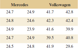
(a) Construct a normal probability plot of each of the data sets. Based on these plots, is it reasonable to assume that they are each drawn from a normal population?
(b) Suppose that it was determined that the lowest observation of the Mercedes data was erroneously recorded and should be 24.6. Furthermore, the lowest observation of the Volkswagen data was also mistaken and should be 39.6. Again construct normal probability plots of each of the data sets with the corrected values. Based on these new plots, is it reasonable to assume that each is drawn from a normal population?
(c) Compare your answers from parts (a) and (b) and comment on the effect of these mistaken observations on the normality assumption.
(d) Using the corrected data from part (b) and a 95% confidence interval, is there evidence to support the claim that the variability in mileage performance is greater for a Volkswagen than for a Mercedes?
(e) Rework part (d) of this problem using an appropriate hypothesis-testing procedure. Did you get the same answer as you did originally? Why?
10-110. ![]() An experiment was conducted to compare the filling capability of packaging equipment at two different wineries. Ten bottles of pinot noir from Ridgecrest Vineyards were randomly selected and measured, as were 10 bottles of pinot noir from Valley View Vineyards. The data are as follows (fill volume is in milliliters):
An experiment was conducted to compare the filling capability of packaging equipment at two different wineries. Ten bottles of pinot noir from Ridgecrest Vineyards were randomly selected and measured, as were 10 bottles of pinot noir from Valley View Vineyards. The data are as follows (fill volume is in milliliters):
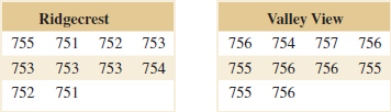
(a) What assumptions are necessary to perform a hypothesis-testing procedure for equality of means of these data? Check these assumptions.
(b) Perform the appropriate hypothesis-testing procedure to determine whether the data support the claim that both wineries will fill bottles to the same mean volume.
(c) Suppose that the true difference in mean fill volume is as much as 2 fluid ounces; did the sample sizes of 10 from each vineyard provide good detection capability when α = 0.05? Explain your answer.
10-111. ![]() A Rockwell hardness-testing machine presses a tip into a test coupon and uses the depth of the resulting depression to indicate hardness. Two different tips are being compared to determine whether each provides the same Rockwell C-scale hardness readings. Nine coupons are tested with both tips being tested on each coupon. The data are shown in the following table.
A Rockwell hardness-testing machine presses a tip into a test coupon and uses the depth of the resulting depression to indicate hardness. Two different tips are being compared to determine whether each provides the same Rockwell C-scale hardness readings. Nine coupons are tested with both tips being tested on each coupon. The data are shown in the following table.
(a) State any assumptions necessary to test the claim that each tip produces the same Rockwell C-scale hardness readings. Check those assumptions for which you have the information.

(b) Apply an appropriate statistical method to determine whether the data support the claim that the difference in Rockwell C-scale hardness readings of the two tips differ significantly from zero.
(c) Suppose that if the two tips differ in mean hardness readings by as much as 1.0, you want the power of the test to be at least 0.9. For an α = 0.01, how many coupons should have been used in the test?
10-112. Two different gauges can be used to measure the depth of bath material in a Hall cell used in smelting aluminum. Each gauge is used once in 15 cells by the same operator.
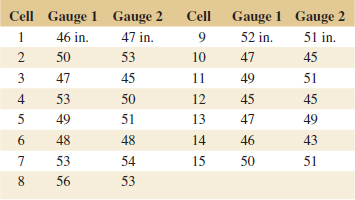
(a) State any assumptions necessary to test the claim that both gauges produce the same mean bath depth readings. Check those assumptions for which you have the information.
(b) Apply an appropriate statistical procedure to determine whether the data support the claim that the two gauges produce different mean bath depth readings.
(c) Suppose that if the two gauges differ in mean bath depth readings by as much as 1.65 inch, you want the power of the test to be at least 0.8. For α = 0.01, how many cells should have been used?
10-113. ![]() An article in the Journal of the Environmental Engineering Division [“Distribution of Toxic Substances in Rivers” (1982, Vol. 108, pp. 639–649)] investigated the concentration of several hydrophobic organic substances in the Wolf River in Tennessee. Measurements on hexachlorobenzene (HCB) in nanograms per liter were taken at different depths downstream of an abandoned dump site. Data for two depths follow:
An article in the Journal of the Environmental Engineering Division [“Distribution of Toxic Substances in Rivers” (1982, Vol. 108, pp. 639–649)] investigated the concentration of several hydrophobic organic substances in the Wolf River in Tennessee. Measurements on hexachlorobenzene (HCB) in nanograms per liter were taken at different depths downstream of an abandoned dump site. Data for two depths follow:
Surface: 3.74, 4.61, 4.00, 4.67, 4.87, 5.12, 4.52, 5.29, 5.74, 5.48
Bottom: 5.44, 6.88, 5.37, 5.44, 5.03, 6.48, 3.89, 5.85, 6.85, 7.16
(a) What assumptions are required to test the claim that mean HCB concentration is the same at both depths? Check those assumptions for which you have the information.
(b) Apply an appropriate procedure to determine whether the data support the claim in part a.
(c) Suppose that the true difference in mean concentrations is 2.0 nanograms per liter. For α = 0.05, what is the power of a statistical test for H0: μ1 = μ2 versus H1: μ1 ≠ μ2?
(d) What sample size would be required to detect a difference of 1.0 nanograms per liter at α = 0.05 if the power must be at least 0.9?
10-114. Consider the foam thickness data from Exercise 10-39. Is there any indication that the variances of foam thickness are different at the two different levels of temperature?
10-115. Consider the grinding force data in Exercise 10-40. Is there any indication that the variances of grinding force are different at the two different levels of temperature?
10-116. Consider the seat belt usage data in Exercise 10-102. Find 95% CIs on the difference in the proportions of seat belt usage for drivers of foreign and domestic cars using both procedures described in this chapter. Compare the lengths of these two intervals and comment on any difference you may observe.
10-117. Consider the unlisted telephone number data in Exercise 10-101. Find 95% CIs on the difference in the proportions of unlisted telephone numbers for Phoenix and Scottsdale residents using both procedures described in this chapter. Compare the lengths of these two intervals and comment on any difference you may observe.
Mind-Expanding Exercises
10-118. Three different pesticides can be used to control pest infestation of grapes. It is suspected that pesticide 3 is more effective than the other two. In a particular vineyard, three different plantings of pinot noir grapes are selected for study. The following results on yield are obtained:
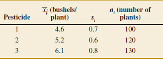
If μi is the true mean yield after treatment with the ith pesticide, you are interested in the quantity
![]()
which measures the difference in mean yields for pesticides 1 and 2 and pesticide 3. If the sample sizes ni are large, the estimator (say, ![]() ) obtained by replacing each individual μi by
) obtained by replacing each individual μi by ![]() i is approximately normal.
i is approximately normal.
(a) Find an approximate 100(1 − x)% large-sample confidence interval for μ.
(b) Do these data support the claim that pesticide 3 is more effective than the other two? Use α = 0.05 in determining your answer.
10-119. Suppose that you wish to test H0: μ1 = μ2 versus H1: μ1 ≠ μ2, where ![]() and
and ![]() are known. The total sample size N is to be determined, and the allocation of observations to the two populations such that n1 + n1 = N is to be made on the basis of cost. If the cost of sampling for populations 1 and 2 are C1 and C2, respectively, find the minimum cost sample sizes that provide a specified variance for the difference in sample means.
are known. The total sample size N is to be determined, and the allocation of observations to the two populations such that n1 + n1 = N is to be made on the basis of cost. If the cost of sampling for populations 1 and 2 are C1 and C2, respectively, find the minimum cost sample sizes that provide a specified variance for the difference in sample means.
10-120. Suppose that you wish to test the hypothesis H0: μ1 = μ2 versus H1: μ1 ≠ μ2, where both variances ![]() and
and ![]() are known. A total of n1 + n2 = N observations can be taken. How should these observations be allocated to the two populations to maximize the probability that H0 will be rejected if H1 is true and μ1 − μ2 = Δ ≠ 0?
are known. A total of n1 + n2 = N observations can be taken. How should these observations be allocated to the two populations to maximize the probability that H0 will be rejected if H1 is true and μ1 − μ2 = Δ ≠ 0?
10-121. Suppose that you wish to test H0: μ = μ0 versus H1: μ ≠ μ0, where the population is normal with known σ. Let 0 < ε < α, and define the critical region so that you will reject H0 if z0 > zε or if z0 < − zα−ε where z0 is the value of the usual test statistic for these hypotheses.
(a) Show that the probability of type I error for this test is α.
(b) Suppose that the true mean is μ1 = μ0 + Δ. Derive an expression for β for the above test.
10-122. Construct a data set for which the paired t-test statistic is very large, indicating that when this analysis is used, the two population means are different, but t0 for the two-sample t-test is very small so that the incorrect analysis would indicate that there is no significant difference for the means.
10-123. In some situations involving proportions, you are interested in the ratio θ = p1/p2 rather than the difference p1 − p2. Let ![]() =
= ![]() 1/
1/![]() 2. It can be shown that ln(
2. It can be shown that ln(![]() ) has an approximate normal distribution with the mean (n/θ) and variance [(n1 − x1)/(n1x1) + (n2 − x2)/(n2x2)]1/2.
) has an approximate normal distribution with the mean (n/θ) and variance [(n1 − x1)/(n1x1) + (n2 − x2)/(n2x2)]1/2.
(a) Use the preceding information to derive a large-sample confidence interval for ln θ.
(b) Show how to find a large-sample CI for θ.
(c) Use the data from the St. John's Wort study in Example 10-16, and find a 95% CI on θ = p1/p2. Provide a practical interpretation for this CI.
10-124. Derive an expression for β for the test of the equality of the variances of two normal distributions. Assume that the two-sided alternative is specified.
Important Terms and Concepts
Comparative experiments
Confidence intervals on differences and ratios
Critical region for a test statistic
Identifying cause and effect
Null and alternative hypotheses
One-sided and two-sided alternative hypotheses
Operating characteristic curves
Paired t-test
Pooled t-test
P-value
Reference distribution for a test statistic
Sample size determination for hypothesis tests and confidence intervals
Statistical hypothesis
Test statistic
Wilcoxon rank-sum test
Sample comparative experiments
Treatments
Randomized experiment
*While we have given the development of this procedure for the case in which the sample sizes could be different, there is an advantage to using equal sample sizes n1 = n2 = n. When the sample sizes are the same from both populations, the t-test is more robust to the assumption of equal variances.