

Tests of Hypotheses for a Single Sample

Chapter Outline
9-1.2 Tests of Statistical Hypotheses
9-1.3 One-Sided and Two-Sided Hypotheses
9-1.4 P-Values in Hypothesis Tests
9-1.5 Connection between Hypothesis Tests and Confidence Intervals
9-1.6 General Procedure for Hypothesis Tests
9-2 Tests on the Mean of a Normal Distribution, Variance Known
9-2.1 Hypothesis Tests on the Mean
9-2.2 Type II Error and Choice of Sample Size
9-3 Tests on the Mean of a Normal Distribution, Variance Unknown
9-3.1 Hypothesis Tests on the Mean
9-3.2 Type II Error and Choice of Sample Size
9-4 Tests on the Variance and Standard Deviation of a Normal Distribution
9-4.1 Hypothesis Tests on the Variance
9-4.2 Type II Error and Choice of Sample Size
9-5 Tests on a Population Proportion
9-5.1 Large-Sample Tests on a Proportion
9-5.2 Type II Error and Choice of Sample Size
9-6 Summary Table of Inference Procedures for a Single Sample
9-7 Testing for Goodness of Fit
9-9.2 The Wilcoxon Signed-Rank Test
INTRODUCTION
In the previous two chapters, we showed how a parameter of a population can be estimated from sample data, using either a point estimate (Chapter 7) or an interval of likely values called a confidence interval (Chapter 8). In many situations, a different type of problem is of interest; there are two competing claims about the value of a parameter, and the engineer must determine which claim is correct. For example, suppose that an engineer is designing an air crew escape system that consists of an ejection seat and a rocket motor that powers the seat. The rocket motor contains a propellant, and for the ejection seat to function properly, the propellant should have a mean burning rate of 50 cm/sec. If the burning rate is too low, the ejection seat may not function properly, leading to an unsafe ejection and possible injury of the pilot. Higher burning rates may imply instability in the propellant or an ejection seat that is too powerful, again leading to possible pilot injury. So the practical engineering question that must be answered is: Does the mean burning rate of the propellant equal 50 cm/sec, or is it some other value (either higher or lower)? This type of question can be answered using a statistical technique called hypothesis testing. This chapter focuses on the basic principles of hypothesis testing and provides techniques for solving the most common types of hypothesis testing problems involving a single sample of data.
![]() Learning Objectives
Learning Objectives
After careful study of this chapter, you should be able to do the following:
- Structure engineering decision-making problems as hypothesis tests
- Test hypotheses on the mean of a normal distribution using either a Z-test or a t-test procedure
- Test hypotheses on the variance or standard deviation of a normal distribution
- Test hypotheses on a population proportion
- Use the P-value approach for making decisions in hypothesis tests
- Compute power and type II error probability, and make sample size selection decisions for tests on means, variances, and proportions
- Explain and use the relationship between confidence intervals and hypothesis tests
- Use the chi-square goodness-of-fit test to check distributional assumptions
- Use contingency table tests
9-1 Hypothesis Testing
9-1.1 STATISTICAL HYPOTHESES
In the previous chapter, we illustrated how to construct a confidence interval estimate of a parameter from sample data. However, many problems in engineering require that we decide which of two competing claims or statements about some parameter is true. The statements are called hypotheses, and the decision-making procedure is called hypothesis testing. This is one of the most useful aspects of statistical inference, because many types of decision-making problems, tests, or experiments in the engineering world can be formulated as hypothesis-testing problems. Furthermore, as we will see, a very close connection exists between hypothesis testing and confidence intervals.
Statistical hypothesis testing and confidence interval estimation of parameters are the fundamental methods used at the data analysis stage of a comparative experiment in which the engineer is interested, for example, in comparing the mean of a population to a specified value. These simple comparative experiments are frequently encountered in practice and provide a good foundation for the more complex experimental design problems that we will discuss in Chapters 13 and 14. In this chapter, we discuss comparative experiments involving a single population, and our focus is on testing hypotheses concerning the parameters of the population.
We now give a formal definition of a statistical hypothesis.
Statistical Hypothesis
A statistical hypothesis is a statement about the parameters of one or more populations.
Because we use probability distributions to represent populations, a statistical hypothesis may also be thought of as a statement about the probability distribution of a random variable. The hypothesis will usually involve one or more parameters of this distribution.
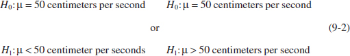
For example, consider the air crew escape system described in the introduction. Suppose that we are interested in the burning rate of the solid propellant. Burning rate is a random variable that can be described by a probability distribution. Suppose that our interest focuses on the mean burning rate (a parameter of this distribution). Specifically, we are interested in deciding whether or not the mean burning rate is 50 centimeters per second. We may express this formally as
![]()
The statement H0: μ = 50 centimeters per second in Equation 9-1 is called the null hypothesis. This is a claim that is initially assumed to be true. The statement H1: μ ≠ 50 centimeters per second is called the alternative hypothesis and it is a statement that condradicts the null hypothesis. Because the alternative hypothesis specifies values of μ that could be either greater or less than 50 centimeters per second, it is called a two-sided alternative hypothesis. In some situations, we may wish to formulate a one-sided alternative hypothesis, as in
We will always state the null hypothesis as an equality claim. However when the alternative hypothesis is stated with the < sign, the implicit claim in the null hypothesis can be taken as ≥ and when the alternative hyphothesis is stated with the > sign, the implicit claim in the null hypothesis can be taken as ≤.
It is important to remember that hypotheses are always statements about the population or distribution under study, not statements about the sample. The value of the population parameter specified in the null hypothesis (50 centimeters per second in the preceding example) is usually determined in one of three ways. First, it may result from past experience or knowledge of the process or even from previous tests or experiments. The objective of hypothesis testing, then, is usually to determine whether the parameter value has changed. Second, this value may be determined from some theory or model regarding the process under study. Here the objective of hypothesis testing is to verify the theory or model. A third situation arises when the value of the population parameter results from external considerations, such as design or engineering specifications, or from contractual obligations. In this situation, the usual objective of hypothesis testing is conformance testing.
A procedure leading to a decision about the null hypothesis is called a test of a hypothesis. Hypothesis-testing procedures rely on using the information in a random sample from the population of interest. If this information is consistent with the null hypothesis, we will not reject it; however, if this information is inconsistent with the null hypothesis, we will conclude that the null hypothesis is false and reject it in favor of the alternative. We emphasize that the truth or falsity of a particular hypothesis can never be known with certainty unless we can examine the entire population. This is usually impossible in most practical situations. Therefore, a hypothesis-testing procedure should be developed with the probability of reaching a wrong conclusion in mind. Testing the hypothesis involves taking a random sample, computing a test statistic from the sample data, and then using the test statistic to make a decision about the null hypothesis.
9-1.2 TESTS OF STATISTICAL HYPOTHESES
To illustrate the general concepts, consider the propellant burning rate problem introduced earlier. The null hypothesis is that the mean burning rate is 50 centimeters per second, and the alternate is that it is not equal to 50 centimeters per second. That is, we wish to test
![]()
Suppose that a sample of n = 10 specimens is tested and that the sample mean burning rate ![]() is observed. The sample mean is an estimate of the true population mean μ. A value of the sample mean
is observed. The sample mean is an estimate of the true population mean μ. A value of the sample mean ![]() that falls close to the hypothesized value of μ = 50 centimeters per second does not conflict with the null hypothesis that the true mean μ is really 50 centimeters per second. On the other hand, a sample mean that is considerably different from 50 centimeters per second is evidence in support of the alternative hypothesis H1. Thus, the sample mean is the test statistic in this case.
that falls close to the hypothesized value of μ = 50 centimeters per second does not conflict with the null hypothesis that the true mean μ is really 50 centimeters per second. On the other hand, a sample mean that is considerably different from 50 centimeters per second is evidence in support of the alternative hypothesis H1. Thus, the sample mean is the test statistic in this case.
The sample mean can take on many different values. Suppose that if 48.5 ≤ ![]() ≤ 51.5, we will not reject the null hypothesis H0: μ = 50, and if either
≤ 51.5, we will not reject the null hypothesis H0: μ = 50, and if either ![]() < 48.5 or
< 48.5 or ![]() > 51.5, we will reject the null hypothesis in favor of the alternative hypothesis H1: μ ≠ 50. This is illustrated in Fig. 9-1. The values of
> 51.5, we will reject the null hypothesis in favor of the alternative hypothesis H1: μ ≠ 50. This is illustrated in Fig. 9-1. The values of ![]() that are less than 48.5 and greater than 51.5 constitute the critical region for the test; all values that are in the interval 48.5 ≤
that are less than 48.5 and greater than 51.5 constitute the critical region for the test; all values that are in the interval 48.5 ≤ ![]() ≤ 51.5 form a region for which we will fail to reject the null hypothesis. By convention, this is usually called the acceptance region. The boundaries between the critical regions and the acceptance region are called the critical values. In our example, the critical values are 48.5 and 51.5. It is customary to state conclusions relative to the null hypothesis H0. Therefore, we reject H0 in favor of H1 if the test statistic falls in the critical region and fail to reject H0 otherwise.
≤ 51.5 form a region for which we will fail to reject the null hypothesis. By convention, this is usually called the acceptance region. The boundaries between the critical regions and the acceptance region are called the critical values. In our example, the critical values are 48.5 and 51.5. It is customary to state conclusions relative to the null hypothesis H0. Therefore, we reject H0 in favor of H1 if the test statistic falls in the critical region and fail to reject H0 otherwise.
This decision procedure can lead to either of two wrong conclusions. For example, the true mean burning rate of the propellant could be equal to 50 centimeters per second. However, for the randomly selected propellant specimens that are tested, we could observe a value of the test statistic ![]() that falls into the critical region. We would then reject the null hypothesis H0 in favor of the alternate H1 when, in fact, H0 is really true. This type of wrong conclusion is called a type I error.
that falls into the critical region. We would then reject the null hypothesis H0 in favor of the alternate H1 when, in fact, H0 is really true. This type of wrong conclusion is called a type I error.
Type I Error
Rejecting the null hypothesis H0 when it is true is defined as a type I error.
Now suppose that the true mean burning rate is different from 50 centimeters per second, yet the sample mean ![]() falls in the acceptance region. In this case, we would fail to reject H0 when it is false. This type of wrong conclusion is called a type II error.
falls in the acceptance region. In this case, we would fail to reject H0 when it is false. This type of wrong conclusion is called a type II error.
Type II Error
Failing to reject the null hypothesis when it is false is defined as a type II error.
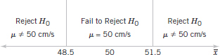
FIGURE 9-1 Decision criteria for testing H0: μ = 50 centimeters per second versus H1: μ ≠ 50 centimeters per second.
Thus, in testing any statistical hypothesis, four different situations determine whether the final decision is correct or in error. These situations are presented in Table 9-1.
Because our decision is based on random variables, probabilities can be associated with the type I and type II errors in Table 9-1. The probability of making a type I error is denoted by the Greek letter α.
Probability of Type I Error
![]()
Sometimes the type I error probability is called the significance level, the α-error, or the size of the test. In the propellant burning rate example, a type I error will occur when either ![]() > 51.5 or
> 51.5 or ![]() < 48.5 when the true mean burning rate really is μ = 50 centimeters per second. Suppose that the standard deviation of burning rate is σ = 2.5 centimeters per second and that the burning rate has a distribution for which the conditions of the central limit theorem apply, so the distribution of the sample mean is approximately normal with mean μ = 50 and standard deviation σ/
< 48.5 when the true mean burning rate really is μ = 50 centimeters per second. Suppose that the standard deviation of burning rate is σ = 2.5 centimeters per second and that the burning rate has a distribution for which the conditions of the central limit theorem apply, so the distribution of the sample mean is approximately normal with mean μ = 50 and standard deviation σ/![]() = 2.5/
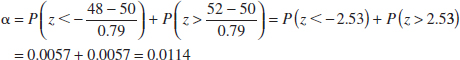
= 2.5/![]() = 0.79. The probability of making a type I error (or the significance level of our test) is equal to the sum of the areas that have been shaded in the tails of the normal distribution in Fig. 9-2. We may find this probability as
= 0.79. The probability of making a type I error (or the significance level of our test) is equal to the sum of the areas that have been shaded in the tails of the normal distribution in Fig. 9-2. We may find this probability as
![]()
Computing the Type I Error Probability
The z-values that correspond to the critical values 48.5 and 51.5 are
![]()
Therefore,
![]()
This is the type I error probability. This implies that 5.74% of all random samples would lead to rejection of the hypothesis H0: μ = 50 centimeters per second when the true mean burning rate is really 50 centimeters per second.
From an inspection of Fig. 9-2, notice that we can reduce α by widening the acceptance region. For example, if we make the critical values 48 and 52, the value of α is
The Impact of Sample Size
We could also reduce α by increasing the sample size. If n = 16, σ/![]() = 2.5/
= 2.5/![]() = 0.625 and using the original critical region from Fig. 9-1, we find
= 0.625 and using the original critical region from Fig. 9-1, we find
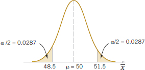
FIGURE 9-2 The critical region for H0: μ = 50 versus H1: μ ≠ 50 and n = 10.
![]() TABLE • 9-1 Decisions in Hypothesis Testing
TABLE • 9-1 Decisions in Hypothesis Testing

Therefore,
![]()
In evaluating a hypothesis-testing procedure, it is also important to examine the probability of a type II error, which we will denote by β. That is,
Probability of Type II Error
![]()
To calculate β (sometimes called the β-error), we must have a specific alternative hypothesis; that is, we must have a particular value of μ. For example, suppose that it is important to reject the null hypothesis H0: μ = 50 whenever the mean burning rate μ is greater than 52 centimeters per second or less than 48 centimeters per second. We could calculate the probability of a type II error β for the values μ = 52 and μ = 48 and use this result to tell us something about how the test procedure would perform. Specifically, how will the test procedure work if we wish to detect, that is, reject H0, for a mean value of μ = 52 or μ = 48? Because of symmetry, it is necessary to evaluate only one of the two cases—say, find the probability of accepting the null hypothesis H0: μ = 50 centimeters per second when the true mean is μ = 52 centimeters per second.
Computing the Probability of Type II Error
Figure 9-3 will help us calculate the probability of type II error β. The normal distribution on the left in Fig. 9-3 is the distribution of the test statistic ![]() when the null hypothesis H0: μ = 50 is true (this is what is meant by the expression “under H0: μ = 50”), and the normal distribution on the right is the distribution of
when the null hypothesis H0: μ = 50 is true (this is what is meant by the expression “under H0: μ = 50”), and the normal distribution on the right is the distribution of ![]() when the alternative hypothesis is true and the value of the mean is 52 (or “under H1: μ = 52”). A type II error will be committed if the sample mean
when the alternative hypothesis is true and the value of the mean is 52 (or “under H1: μ = 52”). A type II error will be committed if the sample mean ![]() falls between 48.5 and 51.5 (the critical region boundaries) when μ = 52. As seen in Fig. 9-3, this is just the probability that 48.5 ≤
falls between 48.5 and 51.5 (the critical region boundaries) when μ = 52. As seen in Fig. 9-3, this is just the probability that 48.5 ≤ ![]() ≤ 51.5 when the true mean is μ = 52, or the shaded area under the normal distribution centered at μ = 52. Therefore, referring to Fig. 9-3, we find that
≤ 51.5 when the true mean is μ = 52, or the shaded area under the normal distribution centered at μ = 52. Therefore, referring to Fig. 9-3, we find that
![]()
The z-values corresponding to 48.5 and 51.5 when μ = 52 are
![]()
Therefore,
![]()
Thus, if we are testing H0: μ = 50 against H1: μ ≠ 50 with n = 10 and the true value of the mean is μ = 52, the probability that we will fail to reject the false null hypothesis is 0.2643. By symmetry, if the true value of the mean is μ = 48, the value of β will also be 0.2643.
The probability of making a type II error β increases rapidly as the true value of μ approaches the hypothesized value. For example, see Fig. 9-4, where the true value of the mean is μ = 50.5 and the hypothesized value is H0: μ = 50. The true value of μ is very close to 50, and the value for β is
![]()
As shown in Fig. 9-4, the z-values corresponding to 48.5 and 51.5 when μ = 50.5 are
![]()
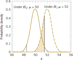
FIGURE 9-3 The probability of type II error when μ = 52 and n = 10.
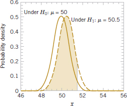
FIGURE 9-4 The probability of type II error when μ = 50.5 and n = 10.
Therefore,
![]()
Thus, the type II error probability is much higher for the case in which the true mean is 50.5 centimeters per second than for the case in which the mean is 52 centimeters per second. Of course, in many practical situations, we would not be as concerned with making a type II error if the mean were “close” to the hypothesized value. We would be much more interested in detecting large differences between the true mean and the value specified in the null hypothesis.
Effect of Sample Size on β
The type II error probability also depends on the sample size n. Suppose that the null hypothesis is H0: μ = 50 centimeters per second and that the true value of the mean is μ = 52. If the sample size is increased from n = 10 to n = 16, the situation of Fig. 9-5 results. The normal distribution on the left is the distribution of ![]() when the mean μ = 50, and the normal distribution on the right is the distribution of
when the mean μ = 50, and the normal distribution on the right is the distribution of ![]() when μ = 52. As shown in Fig. 9-5, the type II error probability is
when μ = 52. As shown in Fig. 9-5, the type II error probability is
![]()
When n = 16, the standard deviation of ![]() is σ/
is σ/![]() = 2.5/
= 2.5/![]() = 0.625, and the z-values corresponding to 48.5 and 51.5 when μ = 52 are
= 0.625, and the z-values corresponding to 48.5 and 51.5 when μ = 52 are
![]()
Therefore,
![]()
Recall that when n = 10 and μ = 52, we found that β = 0.2643; therefore, increasing the sample size results in a decrease in the probability of type II error.
The results from this section and a few other similar calculations are summarized in the following table. The critical values are adjusted to maintain equal α for n = 10 and n = 16. This type of calculation is discussed later in the chapter.
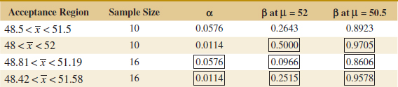
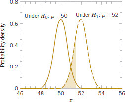
FIGURE 9-5 The probability of type II error when μ = 52 and n = 16.
The results in boxes were not calculated in the text but the reader can easily verify them. This display and the discussion above reveal four important points:
- The size of the critical region, and consequently the probability of a type I error α, can always be reduced by appropriate selection of the critical values.
- Type I and type II errors are related. A decrease in the probability of one type of error always results in an increase in the probability of the other provided that the sample size n does not change.
- An increase in sample size reduces β provided that α is held constant.
- When the null hypothesis is false, β increases as the true value of the parameter approaches the value hypothesized in the null hypothesis. The value of β decreases as the difference between the true mean and the hypothesized value increases.
Generally, the analyst controls the type I error probability α when he or she selects the critical values. Thus, it is usually easy for the analyst to set the type I error probability at (or near) any desired value. Because the analyst can directly control the probability of wrongly rejecting H0, we always think of rejection of the null hypothesis H0 as a strong conclusion.
Because we can control the probability of making a type I error (or significance level), a logical question is what value should be used. The type I error probability is a measure of risk, specifically, the risk of concluding that the null hypothesis is false when it really is not. So, the value of α should be chosen to reflect the consequences (economic, social, etc.) of incorrectly rejecting the null hypothesis. Smaller values of α would reflect more serious consequences and larger values of α would be consistent with less severe consequences. This is often hard to do, so what has evolved in much of scientific and engineering practice is to use the value α = 0.05 in most situations unless information is available that this is an inappropriate choice. In the rocket propellant problem with n = 10, this would correspond to critical values of 48.45 and 51.55.
A widely used procedure in hypothesis testing is to use a type 1 error or significance level of α = 0.05. This value has evolved through experience and may not be appropriate for all situations.
Strong versus Weak Conclusions
On the other hand, the probability of type II error β is not a constant but depends on the true value of the parameter. It also depends on the sample size that we have selected. Because the type II error probability β is a function of both the sample size and the extent to which the null hypothesis H0 is false, it is customary to think of the decision to accept H0 as a weak conclusion unless we know that β is acceptably small. Therefore, rather than saying we “accept H0,” we prefer the terminology “fail to reject H0.” Failing to reject H0 implies that we have not found sufficient evidence to reject H0, that is, to make a strong statement. Failing to reject H0 does not necessarily mean that there is a high probability that H0 is true. It may simply mean that more data are required to reach a strong conclusion. This can have important implications for the formulation of hypotheses.
A useful analog exists between hypothesis testing and a jury trial. In a trial, the defendant is assumed innocent (this is like assuming the null hypothesis to be true). If strong evidence is found to the contrary, the defendant is declared to be guilty (we reject the null hypothesis). If evidence is insufficient, the defendant is declared to be not guilty. This is not the same as proving the defendant innocent and so, like failing to reject the null hypothesis, it is a weak conclusion.
An important concept that we will use is the power of a statistical test.
Power
The power of a statistical test is the probability of rejecting the null hypothesis H0 when the alternative hypothesis is true.
The power is computed as 1 − β, and power can be interpreted as the probability of correctly rejecting a false null hypothesis. We often compare statistical tests by comparing their power properties. For example, consider the propellant burning rate problem when we are testing H0: μ = 50 centimeters per second against H1: μ ≠ 50 centimeters per second. Suppose that the true value of the mean is μ = 52. When n = 10, we found that β = 0.2643, so the power of this test is 1 − β = 1 − 0.2643 = 0.7357 when μ = 52.
Power is a very descriptive and concise measure of the sensitivity of a statistical test when by sensitivity we mean the ability of the test to detect differences. In this case, the sensitivity of the test for detecting the difference between a mean burning rate of 50 centimeters per second and 52 centimeters per second is 0.7357. That is, if the true mean is really 52 centimeters per second, this test will correctly reject H0: μ = 50 and “detect” this difference 73.57% of the time. If this value of power is judged to be too low, the analyst can increase either α or the sample size n.
9-1.3 One-Sided and Two-Sided Hypotheses
In constructing hypotheses, we will always state the null hypothesis as an equality so that the probability of type I error α can be controlled at a specific value. The alternative hypothesis might be either one-sided or two-sided, depending on the conclusion to be drawn if H0 is rejected. If the objective is to make a claim involving statements such as greater than, less than, superior to, exceeds, at least, and so forth, a one-sided alternative is appropriate. If no direction is implied by the claim, or if the claim “not equal to” is to be made, a two-sided alternative should be used.
Example 9-1 Propellant Burning Rate Consider the propellant burning rate problem. Suppose that if the burning rate is less than 50 centimeters per second, we wish to show this with a strong conclusion. The hypotheses should be stated as
![]()
Here the critical region lies in the lower tail of the distribution of ![]() . Because the rejection of H0 is always a strong conclusion, this statement of the hypotheses will produce the desired outcome if H0 is rejected. Notice that, although the null hypothesis is stated with an equals sign, it is understood to include any value of μ not specified by the alternative hypothesis (that is, μ ≤ 50). Therefore, failing to reject H0 does not mean that μ = 50 centimeters per second exactly, but only that we do not have strong evidence in support of H1.
. Because the rejection of H0 is always a strong conclusion, this statement of the hypotheses will produce the desired outcome if H0 is rejected. Notice that, although the null hypothesis is stated with an equals sign, it is understood to include any value of μ not specified by the alternative hypothesis (that is, μ ≤ 50). Therefore, failing to reject H0 does not mean that μ = 50 centimeters per second exactly, but only that we do not have strong evidence in support of H1.
In some real-world problems in which one-sided test procedures are indicated, selecting an appropriate formulation of the alternative hypothesis is occasionally difficult. For example, suppose that a soft-drink beverage bottler purchases 10-ounce bottles from a glass company. The bottler wants to be sure that the bottles meet the specification on mean internal pressure or bursting strength, which for 10-ounce bottles is a minimum strength of 200 psi. The bottler has decided to formulate the decision procedure for a specific lot of bottles as a hypothesis testing problem. There are two possible formulations for this problem, either
![]()
or
![]()
Formulating One-Sided Hypothesis
Consider the formulation in Equation 9-5. If the null hypothesis is rejected, the bottles will be judged satisfactory; if H0 is not rejected, the implication is that the bottles do not conform to specifications and should not be used. Because rejecting H0 is a strong conclusion, this formulation forces the bottle manufacturer to “demonstrate” that the mean bursting strength of the bottles exceeds the specification. Now consider the formulation in Equation 9-6. In this situation, the bottles will be judged satisfactory unless H0 is rejected. That is, we conclude that the bottles are satisfactory unless there is strong evidence to the contrary.
Which formulation is correct, the one of Equation 9-5 or Equation 9-6? The answer is that it depends on the objective of the analysis. For Equation 9-5, there is some probability that H0 will not be rejected (i.e., we would decide that the bottles are not satisfactory) even though the true mean is slightly greater than 200 psi. This formulation implies that we want the bottle manufacturer to demonstrate that the product meets or exceeds our specifications. Such a formulation could be appropriate if the manufacturer has experienced difficulty in meeting specifications in the past or if product safety considerations force us to hold tightly to the 200-psi specification. On the other hand, for the formulation of Equation 9-6, there is some probability that H0 will be accepted and the bottles judged satisfactory, even though the true mean is slightly less than 200 psi. We would conclude that the bottles are unsatisfactory only when there is strong evidence that the mean does not exceed 200 psi, that is, when H0: μ = 200 psi is rejected. This formulation assumes that we are relatively happy with the bottle manufacturer's past performance and that small deviations from the specification of μ ≥ 200 psi are not harmful.
In formulating one-sided alternative hypotheses, we should remember that rejecting H0 is always a strong conclusion. Consequently, we should put the statement about which it is important to make a strong conclusion in the alternative hypothesis. In real-world problems, this will often depend on our point of view and experience with the situation.
9-1.4 P-Values in Hypothesis Tests
One way to report the results of a hypothesis test is to state that the null hypothesis was or was not rejected at a specified α-value or level of significance. This is called fixed significance level testing.
The fixed significance level approach to hypothesis testing is very nice because it leads directly to the concepts of type II error and power, which are of considerable value in determining the appropriate sample sizes to use in hypothesis testing. But the fixed significance level approach does have some disadvantages.
For example, in the propellant problem above, we can say that H0: μ = 50 was rejected at the 0.05 level of significance. This statement of conclusions may be often inadequate because it gives the decision maker no idea about whether the computed value of the test statistic was just barely in the rejection region or whether it was very far into this region. Furthermore, stating the results this way imposes the predefined level of significance on other users of the information. This approach may be unsatisfactory because some decision makers might be uncomfortable with the risks implied by α = 0.05.
To avoid these difficulties, the P-value approach has been adopted widely in practice. The P-value is the probability that the test statistic will take on a value that is at least as extreme as the observed value of the statistic when the null hypothesis H0 is true. Thus, a P-value conveys much information about the weight of evidence against H0, and so a decision maker can draw a conclusion at any specified level of significance. We now give a formal definition of a P-value.
P-Value
The P-value is the smallest level of significance that would lead to rejection of the null hypothesis H0 with the given data.
It is customary to consider the test statistic (and the data) significant when the null hypothesis H0 is rejected; therefore, we may think of the P-value as the smallest level α at which the data are significant. In other words, the P-value is the observed significance level. Once the P-value is known, the decision maker can determine how significant the data are without the data analyst formally imposing a preselected level of significance.
Consider the two-sided hypothesis test for burning rate
![]()
with n = 16 and σ = 2.5. Suppose that the observed sample mean is ![]() = 51.3 centimeters per second. Figure 9-6 is a critical region for this test with the value of
= 51.3 centimeters per second. Figure 9-6 is a critical region for this test with the value of ![]() = 51.3 and the symmetric value 48.7. The P-value of the test is the probability above 51.3 plus the probability below 48.7. The P-value is easy to compute after the test statistic is observed. In this example,
= 51.3 and the symmetric value 48.7. The P-value of the test is the probability above 51.3 plus the probability below 48.7. The P-value is easy to compute after the test statistic is observed. In this example,

The P-value tells us that if the null hypothesis H0 = 50 is true, the probability of obtaining a random sample whose mean is at least as far from 50 as 51.3 (or 48.7) is 0.038. Therefore, an observed sample mean of 51.3 is a fairly rare event if the null hypothesis H0 = 50 is really true. Compared to the “standard” level of significance 0.05, our observed P-value is smaller, so if we were using a fixed significance level of 0.05, the null hypothesis would be rejected. In fact, the null hypothesis H0 = 50 would be rejected at any level of significance greater than or equal to 0.038. This illustrates the previous boxed definition; the P-value is the smallest level of significance that would lead to rejection of H0 = 50.
Operationally, once a P-value is computed, we typically compare it to a predefined significance level to make a decision. Often this predefined significance level is 0.05. However, in presenting results and conclusions, it is standard practice to report the observed P-value along with the decision that is made regarding the null hypothesis.
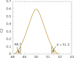
FIGURE 9-6 P-value is the area of the shaded region when ![]() = 51.3.
= 51.3.
Clearly, the P-value provides a measure of the credibility of the null hypothesis. Specifically, it is the risk that we have made an incorrect decision if we reject the null hypothesis H0. The P-value is not the probability that the null hypothesis is false, nor is 1 − P the probability that the null hypothesis is true. The null hypothesis is either true or false (there is no probability associated with this), so the proper interpretation of the P-value is in terms of the risk of wrongly rejecting the null hypothesis H0.
Computing the exact P-value for a statistical test is not always easy. However, most modern statistics software packages report the results of hypothesis testing problems in terms of P-values. We will use the P-value approach extensively.
More About P-Values
We have observed that the procedure for testing a statistical hypothesis consists of drawing a random sample from the population, computing an appropriate statistic, and using the information in that statistic to make a decision regarding the null hypothesis. For example, we have used the sample average in decision making. Because the sample average is a random variable, its value will differ from sample to sample, meaning that the P-value associated with the test procedure will also be a random variable. It also will differ from sample to sample. We are going to use a computer experiment (a simulation) to show how the P-value behaves when the null hypothesis is true and when it is false.
Consider testing the null hypothesis H0: μ = 0 against the alternative hypothesis H0: μ ≠ 0 when we are sampling from a normal population with standard deviation σ = 1. Consider first the case in which the null hypothesis is true and let's suppose that we are going to test the preceding hypotheses using a sample size of n = 10. We wrote a computer program to simulate drawing 10,000 different samples at random from a normal distribution with μ = 0 and σ = 1. Then we calculated the P-values based on the values of the sample averages. Figure 9-7 is a histogram of the P-values obtained from the simulation. Notice that the histogram of the P-values is relatively uniform or flat over the interval from 0 to 1. It turns out that just slightly less than 5% of the P-values are in the interval from 0 to 0.05. It can be shown theoretically that if the null hypothesis is true, the probability distribution of the P-value is exactly uniform on the interval from 0 to 1. Because the null hypothesis is true in this situation, we have demonstrated by simulation that if a test of significance level 0.05 is used, the probability of wrongly rejecting the null hypothesis is (approximately) 0.05.
Now let's see what happens when the null hypothesis is false. We changed the mean of the normal distribution to μ = 1 and repeated the previous computer simulation experiment by drawing another 10,000 samples and computing the P-values. Figure 9-8 is the histogram of the simulated P-values for this situation. Notice that this histogram looks very different from the one in Figure 9-7; there is a tendency for the P-values to stack up near the origin with many more small values between 0 and 0.05 than in the case in which the null hypothesis was true. Not all of the P-values are less than 0.05; those that exceed 0.05 represent type II errors or cases in which the null hypothesis is not rejected at the 0.05 level of significance even though the true mean is not 0.
Finally, Figure 9-8 shows the simulation results when the true value of the mean is even larger; in this case, μ = 2. The simulated P-values are shifted even more toward 0 and concentrated on the left side of the histogram. Generally, as the true mean moves farther and farther away from the hypothesized value of 0 the distribution of the P-values will become more and more concentrated near 0 and fewer and fewer values will exceed 0.05. That is, the farther the mean is from the value specified in the null hypothesis, the higher is the chance that the test procedure will correctly reject the null hypothesis.
9-1.5 CONNECTION BETWEEN HYPOTHESIS TESTS AND CONFIDENCE INTERVALS
A close relationship exists between the test of a hypothesis about any parameter, say θ, and the confidence interval for θ. If [l, u] is a 100(1 − α)% confidence interval for the parameter θ, the test of size α of the hypothesis
![]()
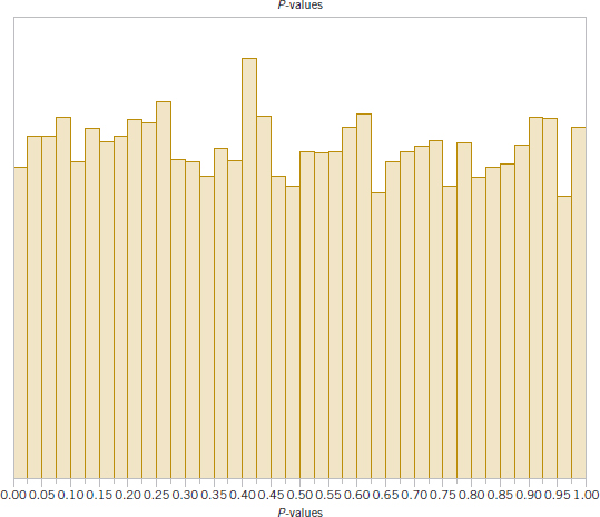
FIGURE 9-7 A P-value simulation when H0: μ = 0 is true.

FIGURE 9-8 A P-value simulation when μ = 1.
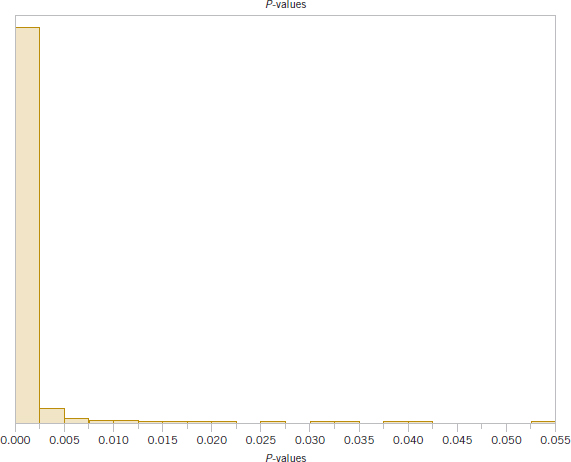
FIGURE 9-9 A P-value simulation when μ = 2.
will lead to rejection of H0 if and only if θ0 is not in the 100(1 − α%) CI [l, u]. As an illustration, consider the escape system propellant problem with ![]() = 51.3, σ = 2.5, and n = 16. The null hypothesis H0: μ = 50 was rejected, using α = 0.05. The 95% two-sided CI on μ can be calculated using Equation 8-7. This CI is 51.3 ± 1.96(2.5/
= 51.3, σ = 2.5, and n = 16. The null hypothesis H0: μ = 50 was rejected, using α = 0.05. The 95% two-sided CI on μ can be calculated using Equation 8-7. This CI is 51.3 ± 1.96(2.5/ ![]() ) and this is 50.075 ≤ μ ≤ 52.525. Because the value μ0 = 50 is not included in this interval, the null hypothesis H0: μ = 50 is rejected.
) and this is 50.075 ≤ μ ≤ 52.525. Because the value μ0 = 50 is not included in this interval, the null hypothesis H0: μ = 50 is rejected.
Although hypothesis tests and CIs are equivalent procedures insofar as decision making or inference about μ is concerned, each provides somewhat different insights. For instance, the confidence interval provides a range of likely values for μ at a stated confidence level whereas hypothesis testing is an easy framework for displaying the risk levels such as the P-value associated with a specific decision. We will continue to illustrate the connection between the two procedures throughout the text.
9-1.6 GENERAL PROCEDURE FOR HYPOTHESIS TESTS
This chapter develops hypothesis-testing procedures for many practical problems. Use of the following sequence of steps in applying hypothesis-testing methodology is recommended.
- Parameter of interest: From the problem context, identify the parameter of interest.
- Null hypothesis, H0: State the null hypothesis, H0.
- Alternative hypothesis, H1: Specify an appropriate alternative hypothesis, H1.
- Test statistic: Determine an appropriate test statistic.
- Reject H0 if: State the rejection criteria for the null hypothesis.
- Computations: Compute any necessary sample quantities, substitute these into the equation for the test statistic, and compute that value.
- Draw conclusions: Decide whether or not H0 should be rejected and report that in the problem context.
Steps 1–4 should be completed prior to examining of the sample data. This sequence of steps will be illustrated in subsequent sections.
In practice, such a formal and (seemingly) rigid procedure is not always necessary. Generally, once the experimenter (or decision maker) has decided on the question of interest and has determined the design of the experiment (that is, how the data are to be collected, how the measurements are to be made, and how many observations are required), only three steps are really required:
- Specify the test statistic to be used (such as Z0).
- Specify the location of the critical region (two-tailed, upper-tailed, or lower-tailed).
- Specify the criteria for rejection (typically, the value of α, or the P-value at which rejection should occur).
These steps are often completed almost simultaneously in solving real-world problems, although we emphasize that it is important to think carefully about each step. That is why we present and use the seven-step process; it seems to reinforce the essentials of the correct approach. Although we may not use it every time in solving real problems, it is a helpful framework when we are first learning about hypothesis testing.
Statistical Versus Practical Significance
We noted previously that reporting the results of a hypothesis test in terms of a P-value is very useful because it conveys more information than just the simple statement “reject H0” or “fail to reject H0.” That is, rejection of H0 at the 0.05 level of significance is much more meaningful if the value of the test statistic is well into the critical region, greatly exceeding the 5% critical value, than if it barely exceeds that value.
Even a very small P-value can be difficult to interpret from a practical viewpoint when we are making decisions because, although a small P-value indicates statistical significance in the sense that H0 should be rejected in favor of H1, the actual departure from H0 that has been detected may have little (if any) practical significance (engineers like to say “engineering significance”). This is particularly true when the sample size n is large.
For example, consider the propellant burning rate problem of Example 9-1 in which we test H0: μ = 50 centimeters per second versus H1: μ ≠ 50 centimeters per second with σ = 2.5. If we suppose that the mean rate is really 50.5 centimeters per second, this is not a serious departure from H0: μ = 50 centimeters per second in the sense that if the mean really is 50.5 centimeters per second, there is no practical observable effect on the performance of the air crew escape system. In other words, concluding that μ = 50 centimeters per second when it is really 50.5 centimeters per second is an inexpensive error and has no practical significance. For a reasonably large sample size, a true value of μ = 50.5 will lead to a sample ![]() that is close to 50.5 centimeters per second, and we would not want this value of
that is close to 50.5 centimeters per second, and we would not want this value of ![]() from the sample to result in rejection of H0. The following display shows the P-value for testing H0: μ = 50 when we observe
from the sample to result in rejection of H0. The following display shows the P-value for testing H0: μ = 50 when we observe ![]() = 50.5 centimeters per second and the power of the test at α = 0.05 when the true mean is 50.5 for various sample sizes n:
= 50.5 centimeters per second and the power of the test at α = 0.05 when the true mean is 50.5 for various sample sizes n:
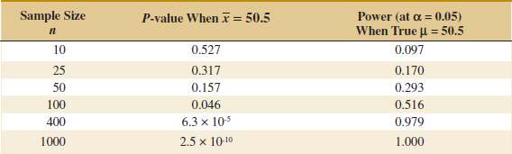
The P-value column in this display indicates that for large sample sizes, the observed sample value of ![]() = 50.5 would strongly suggest that H0: μ = 50 should be rejected, even though the observed sample results imply that from a practical viewpoint, the true mean does not differ much at all from the hypothesized value μ0 = 50. The power column indicates that if we test a hypothesis at a fixed significance level α, and even if there is little practical difference between the true mean and the hypothesized value, a large sample size will almost always lead to rejection of H0. The moral of this demonstration is clear:
= 50.5 would strongly suggest that H0: μ = 50 should be rejected, even though the observed sample results imply that from a practical viewpoint, the true mean does not differ much at all from the hypothesized value μ0 = 50. The power column indicates that if we test a hypothesis at a fixed significance level α, and even if there is little practical difference between the true mean and the hypothesized value, a large sample size will almost always lead to rejection of H0. The moral of this demonstration is clear:
Be careful when interpreting the results from hypothesis testing when the sample size is large because any small departure from the hypothesized value μ0 will probably be detected, even when the difference is of little or no practical significance.
Exercises FOR SECTION 9-1
![]() Problem available in WileyPLUS at instructor's discretion.
Problem available in WileyPLUS at instructor's discretion.
![]() Go Tutorial Tutoring problem available in WileyPLUS at instructor's discretion.
Go Tutorial Tutoring problem available in WileyPLUS at instructor's discretion.
9-1. ![]() State whether each of the following situations is a correctly stated hypothesis testing problem and why.
State whether each of the following situations is a correctly stated hypothesis testing problem and why.
(a) H0: μ = 25, H1: μ ≠ 25
(b) H0: σ > 10, H1: σ = 10
(c) H0: ![]() = 50, H1:
= 50, H1: ![]() ≠ 50
≠ 50
(d) H0: p = 0.1, H1: p = 0.5
(e) H0: s = 30, H1: s > 30
9-2. A semiconductor manufacturer collects data from a new tool and conducts a hypothesis test with the null hypothesis that a critical dimension mean width equals 100 nm. The conclusion is to not reject the null hypothesis. Does this result provide strong evidence that the critical dimension mean equals 100 nm? Explain.
9-3. ![]() The standard deviation of critical dimension thickness in semiconductor manufacturing is σ = 20 nm.
The standard deviation of critical dimension thickness in semiconductor manufacturing is σ = 20 nm.
(a) State the null and alternative hypotheses used to demonstrate that the standard deviation is reduced.
(b) Assume that the previous test does not reject the null hypothesis. Does this result provide strong evidence that the standard deviation has not been reduced? Explain.
9-4. The mean pull-off force of a connector depends on cure time.
(a) State the null and alternative hypotheses used to demonstrate that the pull-off force is below 25 newtons.
(b) Assume that the previous test does not reject the null hypothesis. Does this result provide strong evidence that the pull-off force is greater than or equal to 25 newtons? Explain.
9-5. ![]() A textile fiber manufacturer is investigating a new drapery yarn, which the company claims has a mean thread elongation of 12 kilograms with a standard deviation of 0.5 kilograms. The company wishes to test the hypothesis H0: μ = 12 against H1: μ < 12, using a random sample of four specimens.
A textile fiber manufacturer is investigating a new drapery yarn, which the company claims has a mean thread elongation of 12 kilograms with a standard deviation of 0.5 kilograms. The company wishes to test the hypothesis H0: μ = 12 against H1: μ < 12, using a random sample of four specimens.
(a) What is the type I error probability if the critical region is defined as ![]() < 11.5 kilograms?
< 11.5 kilograms?
(b) Find β for the case in which the true mean elongation is 11.25 kilograms.
(c) Find β for the case in which the true mean is 11.5 kilograms.
9-6. Repeat Exercise 9-5 using a sample size of n = 16 and the same critical region.
9-7. ![]() In Exercise 9-5, find the boundary of the critical region if the type I error probability is
In Exercise 9-5, find the boundary of the critical region if the type I error probability is
(a) α = 0.01 and n = 4
(b) α = 0.05 and n = 4
(c) α = 0.01 and n = 16
(d) α = 0.05 and n = 16
9-8. In Exercise 9-5, calculate the probability of a type II error if the true mean elongation is 11.5 kilograms and
(a) α = 0.05 and n = 4
(b) α = 0.05 and n = 16
(c) Compare the values of β calculated in the previous parts. What conclusion can you draw?
9-9. ![]() In Exercise 9-5, calculate the P-value if the observed statistic is
In Exercise 9-5, calculate the P-value if the observed statistic is
(a) ![]() = 11.25
= 11.25
(b) ![]() = 11.0
= 11.0
(c) ![]() = 11.75
= 11.75
9-10. ![]() The heat evolved in calories per gram of a cement mixture is approximately normally distributed. The mean is thought to be 100, and the standard deviation is 2. You wish to test H0: μ = 100 versus H1: μ ≠ 100 with a sample of n = 9 specimens.
The heat evolved in calories per gram of a cement mixture is approximately normally distributed. The mean is thought to be 100, and the standard deviation is 2. You wish to test H0: μ = 100 versus H1: μ ≠ 100 with a sample of n = 9 specimens.
(a) If the acceptance region is defined as 98.5 ≤ ![]() ≤ 101.5, find the type I error probability α.
≤ 101.5, find the type I error probability α.
(b) Find β for the case in which the true mean heat evolved is 103.
(c) Find β for the case where the true mean heat evolved is 105. This value of β is smaller than the one found in part (b). Why?
9-11. Repeat Exercise 9-10 using a sample size of n = 5 and the same acceptance region.
9-12. In Exercise 9-10, find the boundary of the critical region if the type I error probability is
(a) α = 0.01 and n = 9
(b) α = 0.05 and n = 9
(c) α = 0.01 and n = 5
(d) α = 0.05 and n = 5
9-13. In Exercise 9-10, calculate the probability of a type II error if the true mean heat evolved is 103 and
(a) α = 0.05 and n = 9
(b) α = 0.05 and n = 5
(c) Compare the values of β calculated in the previous parts. What conclusion can you draw?
9-14. ![]() In Exercise 9-10, calculate the P-value if the observed statistic is
In Exercise 9-10, calculate the P-value if the observed statistic is
(a) ![]() = 98
= 98
(b) ![]() = 101
= 101
(c) ![]() = 102
= 102
9-15. ![]() A consumer products company is formulating a new shampoo and is interested in foam height (in millimeters). Foam height is approximately normally distributed and has a standard deviation of 20 millimeters. The company wishes to test H0: μ = 175 millimeters versus H1: μ > 175 millimeters, using the results of n = 10 samples.
A consumer products company is formulating a new shampoo and is interested in foam height (in millimeters). Foam height is approximately normally distributed and has a standard deviation of 20 millimeters. The company wishes to test H0: μ = 175 millimeters versus H1: μ > 175 millimeters, using the results of n = 10 samples.
(a) Find the type I error probability α if the critical region is ![]() > 185.
> 185.
(b) What is the probability of type II error if the true mean foam height is 185 millimeters?
(c) Find β for the true mean of 195 millimeters.
9-16. Repeat Exercise 9-15 assuming that the sample size is n = 16 and the boundary of the critical region is the same.
9-17. ![]() In Exercise 9-15, find the boundary of the critical region if the type I error probability is
In Exercise 9-15, find the boundary of the critical region if the type I error probability is
(a) α = 0.01 and n = 10
(b) α = 0.05 and n = 10
(c) α = 0.01 and n = 16
(d) α = 0.05 and n = 16
9-18. In Exercise 9-15, calculate the probability of a type II error if the true mean foam height is 185 millimeters and
(a) α = 0.05 and n = 10
(b) α = 0.05 and n = 16
(c) Compare the values of β calculated in the previous parts. What conclusion can you draw?
9-19. ![]() In Exercise 9-15, calculate the P-value if the observed statistic is
In Exercise 9-15, calculate the P-value if the observed statistic is
(a) ![]() = 180
= 180
(b) ![]() = 190
= 190
(c) ![]() = 170
= 170
9-20. ![]() A manufacturer is interested in the output voltage of a power supply used in a PC. Output voltage is assumed to be normally distributed with standard deviation 0.25 volt, and the manufacturer wishes to test H0: μ = 5 volts against H1: μ ≠ 5 volts, using n = 8 units.
A manufacturer is interested in the output voltage of a power supply used in a PC. Output voltage is assumed to be normally distributed with standard deviation 0.25 volt, and the manufacturer wishes to test H0: μ = 5 volts against H1: μ ≠ 5 volts, using n = 8 units.
(a) The acceptance region is 4.85 ≤ ![]() ≤ 5.15. Find the value of α.
≤ 5.15. Find the value of α.
(b) Find the power of the test for detecting a true mean output voltage of 5.1 volts.
9-21. Rework Exercise 9-20 when the sample size is 16 and the boundaries of the acceptance region do not change. What impact does the change in sample size have on the results of parts (a) and (b)?
9-22. In Exercise 9-20, find the boundary of the critical region if the type I error probability is
(a) α = 0.01 and n = 8
(b) α = 0.05 and n = 8
(c) α = 0.01 and n = 16
(d) α = 0.05 and n = 16
9-23. In Exercise 9-20, calculate the P-value if the observed statistic is
(a) ![]() = 5.2
= 5.2
(b) ![]() = 4.7
= 4.7
(c) ![]() = 5.1
= 5.1
9-24. In Exercise 9-20, calculate the probability of a type II error if the true mean output is 5.05 volts and
(a) α = 0.05 and n = 10
(b) α = 0.05 and n = 16
(c) Compare the values of β calculated in the previous parts. What conclusion can you draw?
9-25. The proportion of adults living in Tempe, Arizona, who are college graduates is estimated to be p = 0.4. To test this hypothesis, a random sample of 15 Tempe adults is selected. If the number of college graduates is between 4 and 8, the hypothesis will be accepted; otherwise, you will conclude that p ≠ 0.4.
(a) Find the type I error probability for this procedure, assuming that p = 0.4.
(b) Find the probability of committing a type II error if the true proportion is really p = 0.2.
9-26. The proportion of residents in Phoenix favoring the building of toll roads to complete the freeway system is believed to be p = 0.3. If a random sample of 10 residents shows that 1 or fewer favor this proposal, we will conclude that p < 0.3.
(a) Find the probability of type I error if the true proportion is p = 0.3.
(b) Find the probability of committing a type II error with this procedure if p = 0.2.
(c) What is the power of this procedure if the true proportion is p = 0.2?
9-27. ![]() A random sample of 500 registered voters in Phoenix is asked whether they favor the use of oxygenated fuels year-round to reduce air pollution. If more than 400 voters respond positively, we will conclude that more than 60% of the voters favor the use of these fuels.
A random sample of 500 registered voters in Phoenix is asked whether they favor the use of oxygenated fuels year-round to reduce air pollution. If more than 400 voters respond positively, we will conclude that more than 60% of the voters favor the use of these fuels.
(a) Find the probability of type I error if exactly 60% of the voters favor the use of these fuels.
(b) What is the type II error probability β if 75% of the voters favor this action?
Hint: use the normal approximation to the binomial.
9-28. If we plot the probability of accepting H0: μ = μ0 versus various values of μ and connect the points with a smooth curve, we obtain the operating characteristic curve (or the OC curve) of the test procedure. These curves are used extensively in industrial applications of hypothesis testing to display the sensitivity and relative performance of the test. When the true mean is really equal to μ0, the probability of accepting H0 is 1 − α.
(a) Construct an OC curve for Exercise 9-15, using values of the true mean μ of 178, 181, 184, 187, 190, 193, 196, and 199.
(b) Convert the OC curve into a plot of the power function of the test.
9-29. A quality-control inspector is testing a batch of printed circuit boards to see whether they are capable of performing in a high temperature environment. He knows that the boards that will survive will pass all five of the tests with probability 98%. They will pass at least four tests with probability 99%, and they always pass at least three. On the other hand, the boards that will not survive sometimes pass the tests as well. In fact, 3% pass all five tests, and another 20% pass exactly four. The rest pass at most three tests. The inspector decides that if a board passes all five tests, he will classify it as “good.” Otherwise, he'll classify it as “bad.”
(a) What does a type I error mean in this context?
(b) What is the probability of a type I error?
(c) What does a type II error mean here?
(d) What is the probability of a type II error?
9-30. In the quality-control example of Exercise 9-29, the manager says that the probability of a type I error is too large and that it must be no larger than 0.01.
(a) How does this change the rule for deciding whether a board is “good”?
(b) How does this affect the type II error?
(c) Do you think this reduction in type I error is justified? Explain briefly.
9-2 Tests on the Mean of a Normal Distribution, Variance Known
In this section, we consider hypothesis testing about the mean μ of a single normal population where the variance of the population σ2 is known. We will assume that a random sample X1, X2,..., Xn has been taken from the population. Based on our previous discussion, the sample mean ![]() is an unbiased point estimator of μ with variance σ2/n.
is an unbiased point estimator of μ with variance σ2/n.
9-2.1 HYPOTHESIS TESTS ON THE MEAN
Suppose that we wish to test the hypotheses
![]()
where μ0 is a specified constant. We have a random sample X1, X2,..., Xn from a normal population. Because ![]() has a normal distribution (i.e., the sampling distribution of
has a normal distribution (i.e., the sampling distribution of ![]() is normal) with mean μ0 and standard deviation σ/
is normal) with mean μ0 and standard deviation σ/![]() if the null hypothesis is true, we could calculate a P-value or construct a critical region based on the computed value of the sample mean
if the null hypothesis is true, we could calculate a P-value or construct a critical region based on the computed value of the sample mean ![]() , as in Section 9-1.2.
, as in Section 9-1.2.
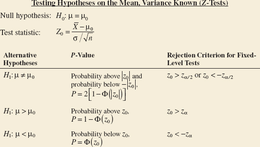
It is usually more convenient to standardize the sample mean and use a test statistic based on the standard normal distribution. That is, the test procedure for H0: μ = μ0 uses the test statistic:
Test Statistic
![]()
If the null hypothesis H0: μ = μ0 is true, E(![]() ) = μ0, and it follows that the distribution of Z0 is the standard normal distribution [denoted N(0,1)].
) = μ0, and it follows that the distribution of Z0 is the standard normal distribution [denoted N(0,1)].
The hypothesis testing procedure is as follows. Take a random sample of size n and compute the value of the sample mean ![]() . To test the null hypothesis using the P-value approach, we would find the probability of observing a value of the sample mean that is at least as extreme as
. To test the null hypothesis using the P-value approach, we would find the probability of observing a value of the sample mean that is at least as extreme as ![]() , given that the null hypothesis is true. The standard normal z-value that corresponds to
, given that the null hypothesis is true. The standard normal z-value that corresponds to ![]() is found from the test statistic in Equation 9-8:
is found from the test statistic in Equation 9-8:
![]()
In terms of the standard normal cumulative distribution function (CDF), the probability we are seeking is 1 − Φ(|z0|). The reason that the argument of the standard normal cdf is |z0| is that the value of z0 could be either positive or negative, depending on the observed sample mean. Because this is a two-tailed test, this is only one-half of the P-value. Therefore, for the two-sided alternative hypothesis, the P-value is
![]()
This is illustrated in Fig. 9-10(a)
Now let's consider the one-sided alternatives. Suppose that we are testing
![]()
Once again, suppose that we have a random sample of size n and that the sample mean is ![]() . We compute the test statistic from Equation 9-8 and obtain z0. Because the test is an upper-tailed test, only values of
. We compute the test statistic from Equation 9-8 and obtain z0. Because the test is an upper-tailed test, only values of ![]() that are greater than μ0 are consistent with the alternative hypothesis. Therefore, the P-value would be the probability that the standard normal random variable is greater than the value of the test statistic z0. This P-value is computed as
that are greater than μ0 are consistent with the alternative hypothesis. Therefore, the P-value would be the probability that the standard normal random variable is greater than the value of the test statistic z0. This P-value is computed as
![]()
This P-value is shown in Fig. 9-10(b).
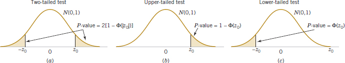
FIGURE 9-10 The P-value for a z-test. (a) The two-sided alternative H1: μ ≠ μ0. (b) The one-sided alternative H1: μ > μ0. (c) The one-sided alternative H1: μ < μ0.
The lower-tailed test involves the hypotheses
![]()
Suppose that we have a random sample of size n and that the sample mean is ![]() . We compute the test statistic from Equation 9-8 and obtain z0. Because the test is a lower-tailed test, only values of
. We compute the test statistic from Equation 9-8 and obtain z0. Because the test is a lower-tailed test, only values of ![]() that are less than μ0 are consistent with the alternative hypothesis. Therefore, the P-value would be the probability that the standard normal random variable is less than the value of the test statistic z0. This P-value is computed as
that are less than μ0 are consistent with the alternative hypothesis. Therefore, the P-value would be the probability that the standard normal random variable is less than the value of the test statistic z0. This P-value is computed as
![]()
and shown in Fig. 9-10(c)
The reference distribution for this test is the standard normal distribution. The test is usually called a z-test.
We can also use the fixed significance level approach with the z-test. The only thing we have to do is determine where to place the critical regions for the two-sided and one-sided alternative hypotheses. First consider the two-sided alternative in Equation 9-10. Now if H0: μ = μ0 is true, the probability is 1 − α that the test statistic Z0 falls between − zα/2 and zα/2 where zα/2 is the 100α/2 percentage point of the standard normal distribution. The regions associated with zα/2 and − zα/2 are illustrated in Fig. 9-11(a). Note that the probability is α that the test statistic Z0 will fall in the region Z0 > zα/2 or Z0 < − zα/2, when H0: μ = μ0 is true. Clearly, a sample producing a value of the test statistic that falls in the tails of the distribution of Z0 would be unusual if H0: μ = μ0 is true; therefore, it is an indication that H0 is false. Thus, we should reject H0 if either
![]()
or
![]()
and we should fail to reject H0 if
![]()
Equations 9-14 and 9-15 define the critical region or rejection region for the test. The type I error probability for this test procedure is α.
We may also develop fixed significance level testing procedures for the one-sided alternatives. Consider the upper-tailed case in Equation 9-10.
In defining the critical region for this test, we observe that a negative value of the test statistic Z0 would never lead us to conclude that H0: μ = μ0 is false. Therefore, we would place the critical region in the upper tail of the standard normal distribution and reject H0 if the computed value z0 is too large. Refer to Fig. 9-11(b). That is, we would reject H0 if
![]()
Similarly, to test the lower-tailed case in Equation 9-12, we would calculate the test statistic Z0 and reject H0 if the value of Z0 is too small. That is, the critical region is in the lower tail of the standard normal distribution as in Fig. 9-11(c), and we reject H0 if
![]()
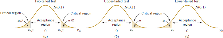
FIGURE 9-11 The distribution of Z0 when H1: μ = μ0 is true with critical region for (a) The two-sided alternative H1: μ ≠ μ0 (b) The one-sided alternative H1: μ > μ0. (c) The one-sided alternative H1: μ < μ0.
Summary of Tests on the Mean, Variance Known
The P-values and critical regions for these situations are shown in Figs. 9-10 and 9-11.
In general, understanding the critical reason and the test procedure is easier when the test statistic is Z0 rather than ![]() . However, the same critical region can always be written in terms of the computed value of the sample mean
. However, the same critical region can always be written in terms of the computed value of the sample mean ![]() . A procedure identical to the preceding fixed significance level test is as follows:
. A procedure identical to the preceding fixed significance level test is as follows:
![]()
where
![]()
Example 9-2 Propellant Burning Rate Air crew escape systems are powered by a solid propellant. The burning rate of this propellant is an important product characteristic. Specifications require that the mean burning rate must be 50 centimeters per second. We know that the standard deviation of burning rate is σ = 2 centimeters per second. The experimenter decides to specify a type I error probability or significance level of α = 0.05 and selects a random sample of n = 25 and obtains a sample average burning rate of ![]() = 51.3 centimeters per second. What conclusions should be drawn?
= 51.3 centimeters per second. What conclusions should be drawn?
We may solve this problem by following the seven-step procedure outlined in Section 9-16. This results in
- Parameter of interest: The parameter of interest is μ, the mean burning rate.
- Null hypothesis: H0: μ = 50 centimeters per second
- Alternative hypothesis: H1: μ ≠ 50 centimeters per second
- Test statistic: The test statistic is

- Reject H0 if: Reject H0 if the P-value is less than 0.05. To use a fixed significance level test, the boundaries of the critical region would be z0.025 = 1.96 and −z0.025 = −1.96.
- Computations: Because
 = 51.3 and σ = 2,
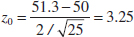
- Conclusion: Because the P-value = 2[1 − Φ(3.25)] = 0.0012 we reject H0: μ = 50 at the 0.05 level of significance.
Practical Interpretation: We conclude that the mean burning rate differs from 50 centimeters per second, based on a sample of 25 measurements. In fact, there is strong evidence that the mean burning rate exceeds 50 centimeters per second.
9-2.2 TYPE II ERROR AND CHOICE OF SAMPLE SIZE
In testing hypotheses, the analyst directly selects the type I error probability. However, the probability of type II error β depends on the choice of sample size. In this section, we will show how to calculate the probability of type II error β. We will also show how to select the sample size to obtain a specified value of β.
Finding the Probability of Type II Error β
Consider the two-sided hypotheses
![]()
Suppose that the null hypothesis is false and that the true value of the mean is μ = μ0 + δ, say, where δ > 0. The test statistic Z0 is
![]()
Therefore, the distribution of Z0 when H1 is true is
![]()
The distribution of the test statistic Z0 under both the null hypothesis H0 and the alternate hypothesis H1 is shown in Fig. 9-9. From examining this figure, we note that if H1 is true, a type II error will be made only if − zα/2 ≤ Z0 ≤ zα/2 where Z0 ~ N(δ![]() /σ, 1). That is, the probability of the type II error β is the probability that Z0 falls between − zα/2 and zα/2 given that H1 is true. This probability is shown as the shaded portion of Fig. 9-12. Expressed mathematically, this probability is
/σ, 1). That is, the probability of the type II error β is the probability that Z0 falls between − zα/2 and zα/2 given that H1 is true. This probability is shown as the shaded portion of Fig. 9-12. Expressed mathematically, this probability is
Probability of a Type II Error for a Two-Sided Test on the Mean, Variance Known
![]()
where Φ(z) denotes the probability to the left of z in the standard normal distribution. Note that Equation 9-20 was obtained by evaluating the probability that Z0 falls in the interval [− zα/2, zα/2] when H1 is true. Furthermore, note that Equation 9-20 also holds if δ < 0, because of the symmetry of the normal distribution. It is also possible to derive an equation similar to Equation 9-20 for a one-sided alternative hypothesis.

FIGURE 9-12 The distribution of Z0 under H0 and H1.
Sample Size Formulas
One may easily obtain formulas that determine the appropriate sample size to obtain a particular value of β for a given Δ and α. For the two-sided alternative hypothesis, we know from Equation 9-20 that
![]()
or, if δ > 0,
![]()
because Φ(−zα/2 − δ![]() /σ)
/σ) ![]() 0 when δ is positive. Let zβ be the 100β upper percentile of the standard normal distribution. Then, β = Φ(−zβ). From Equation 9-21,
0 when δ is positive. Let zβ be the 100β upper percentile of the standard normal distribution. Then, β = Φ(−zβ). From Equation 9-21,
![]()
or
Sample Size for a Two-Sided Test on the Mean, Variance Known
![]()
If n is not an integer, the convention is to round the sample size up to the next integer. This approximation is good when Φ(−zα/2 − δ![]() /σ) is small compared to β. For either of the one-sided alternative hypotheses, the sample size required to produce a specified type II error with probability β given δ and α is
/σ) is small compared to β. For either of the one-sided alternative hypotheses, the sample size required to produce a specified type II error with probability β given δ and α is
Sample Size for a One-Sided Test on the Mean, Variance Known
![]()
Example 9-3 Propellant Burning Rate Type II Error Consider the rocket propellant problem of Example 9-2. Suppose that the true burning rate is 49 centimeters per second. What is β for the two-sided test with α = 0.05, σ = 2, and n = 25?
Here δ = 1 and zα/2 = 1.96. From Equation 9-20,
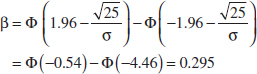
The probability is about 0.3 that this difference from 50 centimeters per second will not be detected. That is, the probability is about 0.3 that the test will fail to reject the null hypothesis when the true burning rate is 49 centimeters per second.
Practical Interpretation: A sample size of n = 25 results in reasonable, but not great, power = 1 − β = 1 − 0.3 = 0.70.
Suppose that the analyst wishes to design the test so that if the true mean burning rate differs from 50 centimeters per second by as much as 1 centimeter per second, the test will detect this (i.e., reject H0: μ = 50) with a high probability, say, 0.90. Now we note that σ = 2, δ = 51 − 50 = 1, α = 0.05, and β = 0.10. Because zα/2 = z0.025 = 1.96 and zβ = z0.10 = 1.28, the sample size required to detect this departure from H0: μ = 50 is found by Equation 9-22 as
![]()
The approximation is good here, because Φ(−zα/2 − δ![]() /σ) = Φ(−1.96 − (1)
/σ) = Φ(−1.96 − (1)![]() /2) = Φ(−5.20)
/2) = Φ(−5.20) ![]() 0, which is small relative to β.
0, which is small relative to β.
Practical Interpretation: To achieve a much higher power of 0.90, you will need a considerably large sample size, n = 42 instead of n = 25.
Using Operating Characteristic Curves
When performing sample size or type II error calculations, it is sometimes more convenient to use the operating characteristic (OC) curves in Appendix Charts VIIa & b. These curves plot β as calculated from Equation 9-20 against a parameter d for various sample sizes n. Curves are provided for both α = 0.05 and α = 0.01. The parameter d is defined as
![]()
so one set of operating characteristic curves can be used for all problems regardless of the values of μ0 and σ. From examining the operating characteristic curves or from Equation 9-20 and Fig. 9-9, we note that
- The farther the true value of the mean μ is from μ0, the smaller the probability of type II error β for a given n and α. That is, we see that for a specified sample size and α, large differences in the mean are easier to detect than small ones.
- For a given δ and α, the probability of type II error β decreases as n increases. That is, to detect a specified difference δ in the mean, we may make the test more powerful by increasing the sample size.
Example 9-4 Propellant Burning Rate Type II Error From OC Curve Consider the propellant problem in Example 9-2. Suppose that the analyst is concerned about the probability of type II error if the true mean burning rate is μ = 51 centimeters per second. We may use the operating characteristic curves to find β. Note that δ = 51 − 50 = 1, n = 25, σ = 2, and α = 0.05. Then using Equation 9-24 gives
![]()
and from Appendix Chart VIIa with n = 25, we find that β = 0.30. That is, if the true mean burning rate is μ = 51 centimeters per second, there is approximately a 30% chance that this will not be detected by the test with n = 25.
Example 9-5 Propellant Burning Rate Sample Size From OC Curve Once again, consider the propellant problem in Example 9-2. Suppose that the analyst would like to design the test so that if the true mean burning rate differs from 50 centimeters per second by as much as 1 centimeter per second, the test will detect this (i.e., reject H0: μ = 50) with a high probability, say, 0.90. This is exactly the same requirement as in Example 9-3 in which we used Equation 9-22 to find the required sample size to be n = 42. The operating characteristic curves can also be used to find the sample size for this test. Because d = |μ − μ0|/σ = 1/2, α = 0.05, and β = 0.10, we find from Appendix Chart VIIa that the required sample size is approximately n = 40. This closely agrees with the sample size calculated from Equation 9-22.
In general, the operating characteristic curves involve three parameters: β, d, and n. Given any two of these parameters, the value of the third can be determined. There are two typical applications of these curves:
Use of OC Curves
- For a given n and d, find β (as illustrated in Example 9-4). Analysts often encounter this kind of problem when they are concerned about the sensitivity of an experiment already performed, or when sample size is restricted by economic or other factors.
- For a given β and d, find n. This was illustrated in Example 9-5. Analysts usually encounter this kind of problem when they have the opportunity to select the sample size at the outset of the experiment.
Operating characteristic curves are given in Appendix Charts VIIc and VIId for the one-sided alternatives. If the alternative hypothesis is either H1: μ > μ0 or H1: μ < μ0, the abscissa scale on these charts is
![]()
Using the Computer
Many statistics software packages can calculate sample sizes and type II error probabilities. To illustrate, here are some typical computer calculations for the propellant burning rate problem:
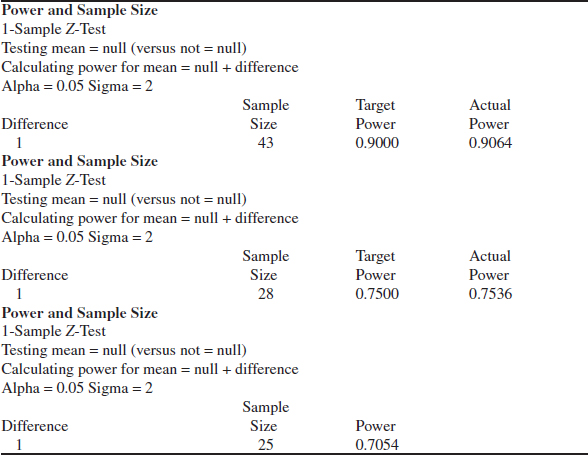
In the first part of the boxed display, we worked Example 9-3, that is, to find the sample size n that would allow detection of a difference from μ0 = 50 of 1 centimeter per second with power of 0.9 and α = 0.05. The answer, n = 43, agrees closely with the calculated value from Equation 9-22 in Example 9-3, which was n = 42. The difference is due to the software's use of a value of zβ that has more than two decimal places. The second part of the computer output relaxes the power requirement to 0.75. Note that the effect is to reduce the required sample size to n = 28. The third part of the output is the solution to Example 9-4 for which we wish to determine the type II error probability of (β) or the power = 1 − β for the sample size n = 25. Note that software computes the power to be 0.7054, which agrees closely with the answer obtained from the OC curve in Example 9-4. Generally, however, the computer calculations will be more accurate than visually reading values from an OC curve.
9-2.3 LARGE-SAMPLE TEST
We have developed the test procedure for the null hypothesis H0: μ = μ0 assuming that the population is normally distributed and that σ2 is known. In many if not most practical situations, σ2 will be unknown. Furthermore, we may not be certain that the population is well modeled by a normal distribution. In these situations, if n is large (say, n > 40), the sample standard deviation s can be substituted for σ in the test procedures with little effect. Thus, although we have given a test for the mean of a normal distribution with known σ2, it can be easily converted into a large-sample test procedure for unknown σ2 that is valid regardless of the form of the distribution of the population. This large-sample test relies on the central limit theorem just as the large-sample confidence interval on μ that was presented in the previous chapter did. Exact treatment of the case in which the population is normal, σ2 is unknown, and n is small involves use of the t distribution and will be deferred until Section 9-3.
Exercises FOR SECTION 9-2
![]() Problem available in WileyPLUS at instructor's discretion.
Problem available in WileyPLUS at instructor's discretion.
![]() Go Tutorial Tutoring problem available in WileyPLUS at instructor's discretion.
Go Tutorial Tutoring problem available in WileyPLUS at instructor's discretion.
9-31. State the null and alternative hypothesis in each case.
(a) A hypothesis test will be used to potentially provide evidence that the population mean is more than 10.
(b) A hypothesis test will be used to potentially provide evidence that the population mean is not equal to 7.
(c) A hypothesis test will be used to potentially provide evidence that the population mean is less than 5.
9-32. ![]() A hypothesis will be used to test that a population mean equals 7 against the alternative that the population mean does not equal 7 with known variance σ. What are the critical values for the test statistic Z0 for the following significance levels?
A hypothesis will be used to test that a population mean equals 7 against the alternative that the population mean does not equal 7 with known variance σ. What are the critical values for the test statistic Z0 for the following significance levels?
(a) 0.01
(b) 0.05
(c) 0.10
9-33. A hypothesis will be used to test that a population mean equals 10 against the alternative that the population mean is more than 10 with known variance σ. What is the critical value for the test statistic Z0 for the following significance levels?
(a) 0.01
(b) 0.05
(c) 0.10
9-34. ![]() A hypothesis will be used to test that a population mean equals 5 against the alternative that the population mean is less than 5 with known variance σ. What is the critical value for the test statistic Z0 for the following significance levels?
A hypothesis will be used to test that a population mean equals 5 against the alternative that the population mean is less than 5 with known variance σ. What is the critical value for the test statistic Z0 for the following significance levels?
(a) 0.01
(b) 0.05
(c) 0.10
9-35. ![]() For the hypothesis test H0:μ = 7 against H1:μ ≠ 7 and variance known, calculate the P-value for each of the following test statistics.
For the hypothesis test H0:μ = 7 against H1:μ ≠ 7 and variance known, calculate the P-value for each of the following test statistics.
(a) z0 = 2.05
(b) z0 = −1.84
(c) z0 = 0.4
9-36. ![]() For the hypothesis test H0: μ = 10 against H1: μ > 10 and variance known, calculate the P-value for each of the following test statistics.
For the hypothesis test H0: μ = 10 against H1: μ > 10 and variance known, calculate the P-value for each of the following test statistics.
(a) z0 = 2.05
(b) z0 = −1.84
(c) z0 = 0.4
9-37. For the hypothesis test H0: μ = 5 against H1: μ < 5 and variance known, calculate the P-value for each of the following test statistics.
(a) z0 = 2.05
(b) z0 = −1.84
(c) z0 = 0.4
9-38. Output from a software package follows:
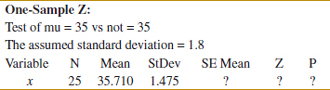
(a) Fill in the missing items. What conclusions would you draw?
(b) Is this a one-sided or a two-sided test?
(c) Use the normal table and the preceding data to construct a 95% two-sided CI on the mean.
(d) What would the P-value be if the alternative hypothesis is H1: μ > 35?
9-39. Output from a software package follows:
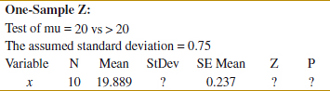
(a) Fill in the missing items. What conclusions would you draw?
(b) Is this a one-sided or a two-sided test?
(c) Use the normal table and the preceding data to construct a 95% two-sided CI on the mean.
(d) What would the P-value be if the alternative hypothesis is H1: μ ≠ 20?
9-40. Output from a software package follows:
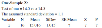
(a) Fill in the missing items. What conclusions would you draw?
(b) Is this a one-sided or a two-sided test?
(c) Use the normal table and the preceding data to construct a 95% lower bound on the mean.
(d) What would the P-value be if the alternative hypothesis is H1: μ ≠ 14.5?
9-41. Output from a software package follows:
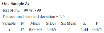
(a) Fill in the missing items. What conclusions would you draw?
(b) Is this a one-sided or a two-sided test?
(c) If the hypothesis had been H0: μ = 98 versus H0: μ > 98, would you reject the null hypothesis at the 0.05 level of significance? Can you answer this without referring to the normal table?
(d) Use the normal table and the preceding data to construct a 95% lower bound on the mean.
(e) What would the P-value be if the alternative hypothesis is H1: μ ≠ 99?
9-42. ![]() The mean water temperature downstream from a discharge pipe at a power plant cooling tower should be no more than 100°F. Past experience has indicated that the standard deviation of temperature is 2°F. The water temperature is measured on nine randomly chosen days, and the average temperature is found to be 98°F.
The mean water temperature downstream from a discharge pipe at a power plant cooling tower should be no more than 100°F. Past experience has indicated that the standard deviation of temperature is 2°F. The water temperature is measured on nine randomly chosen days, and the average temperature is found to be 98°F.
(a) Is there evidence that the water temperature is acceptable at α = 0.05?
(b) What is the P-value for this test?
(c) What is the probability of accepting the null hypothesis at α = 0.05 if the water has a true mean temperature of 104°F?
9-43. A manufacturer produces crankshafts for an automobile engine. The crankshafts wear after 100,000 miles (0.0001 inch) is of interest because it is likely to have an impact on warranty claims. A random sample of n = 15 shafts is tested and ![]() = 2.78. It is known that σ = 0.9 and that wear is normally distributed.
= 2.78. It is known that σ = 0.9 and that wear is normally distributed.
(a) Test H0: μ = 3 versus H1: μ ≠ 3 using α = 0.05.
(b) What is the power of this test if μ = 3.25?
(c) What sample size would be required to detect a true mean of 3.75 if we wanted the power to be at least 0.9?
9-44. ![]() A melting point test of n = 10 samples of a binder used in manufacturing a rocket propellant resulted in
A melting point test of n = 10 samples of a binder used in manufacturing a rocket propellant resulted in ![]() = 154.2°F. Assume that the melting point is normally distributed with σ = 1.5° F.
= 154.2°F. Assume that the melting point is normally distributed with σ = 1.5° F.
(a) Test H0: μ = 155 versus H1: μ ≠ 155 using α = 0.01.
(b) What is the P-value for this test?
(c) What is the β-error if the true mean is μ = 150?
(d) What value of n would be required if we want β < 0.1 when μ = 150? Assume that α = 0.01.
9-45. ![]() The life in hours of a battery is known to be approximately normally distributed with standard deviation σ = 1.25 hours. A random sample of 10 batteries has a mean life of
The life in hours of a battery is known to be approximately normally distributed with standard deviation σ = 1.25 hours. A random sample of 10 batteries has a mean life of ![]() = 40.5 hours.
= 40.5 hours.
(a) Is there evidence to support the claim that battery life exceeds 40 hours? Use α = 0.05.
(b) What is the P-value for the test in part (a)?
(c) What is the β-error for the test in part (a) if the true mean life is 42 hours?
(d) What sample size would be required to ensure that β does not exceed 0.10 if the true mean life is 44 hours?
(e) Explain how you could answer the question in part (a) by calculating an appropriate confidence bound on life.
9-46. An engineer who is studying the tensile strength of a steel alloy intended for use in golf club shafts knows that tensile strength is approximately normally distributed with σ = 60 psi. A random sample of 12 specimens has a mean tensile strength of ![]() = 3450 psi.
= 3450 psi.
(a) Test the hypothesis that mean strength is 3500 psi. Use α = 0.01.
(b) What is the smallest level of significance at which you would be willing to reject the null hypothesis?
(c) What is the β-error for the test in part (a) if the true mean is 3470?
(d) Suppose that you wanted to reject the null hypothesis with probability at least 0.8 if mean strength μ = 3470. What sample size should be used?
(e) Explain how you could answer the question in part (a) with a two-sided confidence interval on mean tensile strength.
9-47. ![]() Supercavitation is a propulsion technology for undersea vehicles that can greatly increase their speed. It occurs above approximately 50 meters per second when pressure drops sufficiently to allow the water to dissociate into water vapor, forming a gas bubble behind the vehicle. When the gas bubble completely encloses the vehicle, supercavitation is said to occur. Eight tests were conducted on a scale model of an undersea vehicle in a towing basin with the average observed speed
Supercavitation is a propulsion technology for undersea vehicles that can greatly increase their speed. It occurs above approximately 50 meters per second when pressure drops sufficiently to allow the water to dissociate into water vapor, forming a gas bubble behind the vehicle. When the gas bubble completely encloses the vehicle, supercavitation is said to occur. Eight tests were conducted on a scale model of an undersea vehicle in a towing basin with the average observed speed ![]() = 102.2 meters per second. Assume that speed is normally distributed with known standard deviation σ = 4 meters per second.
= 102.2 meters per second. Assume that speed is normally distributed with known standard deviation σ = 4 meters per second.
(a) Test the hypothesis H0:μ = 100 versus H1: μ < 100 using α = 0.05.
(b) What is the P-value for the test in part (a)?
(c) Compute the power of the test if the true mean speed is as low as 95 meters per second.
(d) What sample size would be required to detect a true mean speed as low as 95 meters per second if you wanted the power of the test to be at least 0.85?
(e) Explain how the question in part (a) could be answered by constructing a one-sided confidence bound on the mean speed.
9-48. ![]() A bearing used in an automotive application is supposed to have a nominal inside diameter of 1.5 inches. A random sample of 25 bearings is selected, and the average inside diameter of these bearings is 1.4975 inches. Bearing diameter is known to be normally distributed with standard deviation σ = 0.01 inch.
A bearing used in an automotive application is supposed to have a nominal inside diameter of 1.5 inches. A random sample of 25 bearings is selected, and the average inside diameter of these bearings is 1.4975 inches. Bearing diameter is known to be normally distributed with standard deviation σ = 0.01 inch.
(a) Test the hypothesis H0:μ = 1.5 versus H1: μ ≠ 1.5 using α = 0.01.
(b) What is the P-value for the test in part (a)?
(c) Compute the power of the test if the true mean diameter is 1.495 inches.
(d) What sample size would be required to detect a true mean diameter as low as 1.495 inches if you wanted the power of the test to be at least 0.9?
(e) Explain how the question in part (a) could be answered by constructing a two-sided confidence interval on the mean diameter.
9-49. ![]() Medical researchers have developed a new artificial heart constructed primarily of titanium and plastic. The heart will last and operate almost indefinitely once it is implanted in the patient's body, but the battery pack needs to be recharged about every four hours. A random sample of 50 battery packs is selected and subjected to a life test. The average life of these batteries is 4.05 hours. Assume that battery life is normally distributed with standard deviation σ = 0.2 hour.
Medical researchers have developed a new artificial heart constructed primarily of titanium and plastic. The heart will last and operate almost indefinitely once it is implanted in the patient's body, but the battery pack needs to be recharged about every four hours. A random sample of 50 battery packs is selected and subjected to a life test. The average life of these batteries is 4.05 hours. Assume that battery life is normally distributed with standard deviation σ = 0.2 hour.
(a) Is there evidence to support the claim that mean battery life exceeds 4 hours? Use α = 0.05.
(b) What is the P-value for the test in part (a)?
(c) Compute the power of the test if the true mean battery life is 4.5 hours.
(d) What sample size would be required to detect a true mean battery life of 4.5 hours if you wanted the power of the test to be at least 0.9?
(e) Explain how the question in part (a) could be answered by constructing a one-sided confidence bound on the mean life.
9-50. Humans are known to have a mean gestation period of 280 days (from last menstruation) with a standard deviation of about 9 days. A hospital wondered whether there was any evidence that their patients were at risk for giving birth prematurely. In a random sample of 70 women, the average gestation time was 274.3 days.
(a) Is the alternative hypothesis one- or two-sided?
(b) Test the null hypothesis at α = 0.05.
(c) What is the P-value of the test statistic?
9-51. The bacterial strain Acinetobacter has been tested for its adhesion properties. A sample of five measurements gave readings of 2.69, 5.76, 2.67, 1.62 and 4.12 dyne-cm2. Assume that the standard deviation is known to be 0.66 dyne-cm2 and that the scientists are interested in high adhesion (at least 2.5 dyne-cm2).
(a) Should the alternative hypothesis be one-sided or two-sided?
(b) Test the hypothesis that the mean adhesion is 2.5 dyne-cm2.
(c) What is the P-value of the test statistic?
9-3 Tests on the Mean of a Normal Distribution, Variance Unknown
9-3.1 HYPOTHESIS TESTS ON THE MEAN
We now consider the case of hypothesis testing on the mean of a population with unknown variance σ2. The situation is analogous to the one in Section 8-2 where we considered a confidence interval on the mean for the same situation. As in that section, the validity of the test procedure we will describe rests on the assumption that the population distribution is at least approximately normal. The important result on which the test procedure relies is that if X1, X2,..., Xn is a random sample from a normal distribution with mean μ and variance σ2, the random variable
has a t distribution with n − 1 degrees of freedom. Recall that we used this result in Section 8-2 to devise the t-confidence interval for μ. Now consider testing the hypotheses
![]()
We will use the test statistic:
Test Statistic
![]()
If the null hypothesis is true, T0 has a t distribution with n − 1 degrees of freedom. When we know the distribution of the test statistic when H0 is true (this is often called the reference distribution or the null distribution), we can calculate the P-value from this distribution, or, if we use a fixed significance level approach, we can locate the critical region to control the type I error probability at the desired level.
To test H0: μ = μ0 against the two-sided alternative H1: μ ≠ μ0, the value of the test statistic t0 in Equation 9-26 is calculated, and the P-value is found from the t distribution with n − 1 degrees of freedom. Because the test is two-tailed, the P-value is the sum of the probabilities in the two tails of the t distribution. Refer to Fig. 9-13(a). The P-value is the probability above |t0| plus the probability below. Because the t distribution is symmetric around zero, a simple way to write this is
![]()
A small P-value is evidence against H0, so if P is of sufficiently small value (typically < 0.05), reject the null hypothesis.
For the one-sided alternative hypotheses
![]()
we calculate the test statistic t0 from Equation 9-26 and calculate the P-value as
![]()
For the other one-sided alternative
![]()
we calculate the P-value as
![]()
Figure 9-13(b) and (c) show how these P-values are calculated.
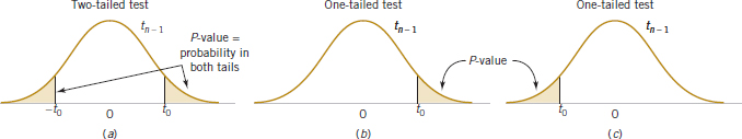
FIGURE 9-13 Calculating the P-value for a t-test: (a) H1: μ ≠ μ0, (b) H1: μ > μ0, (c) H1: μ < μ0.

FIGURE 9-14 P-value for t0 = 2.8; an upper-tailed test is shown to be between 0.005 and 0.01.
Statistics software packages calculate and display P-values. However, in working problems by hand, it is useful to be able to find the P-value for a t-test. Because the t-table in Appendix A Table V contains only 10 critical values for each t distribution, determining the exact P-value from this table is usually impossible. Fortunately, it is easy to find lower and upper bounds on the P-value by using this table.
To illustrate, suppose that we are conducting an upper-tailed t-test (so H1: μ > μ0) with 14 degrees of freedom. The relevant critical values from Appendix A Table II are as follows:
![]()
After calculating the test statistic, we find that t0 = 2.8. Now t0 = 2.8 is between two tabulated values, 2.624 and 2.977. Therefore, the P-value must be between 0.01 and 0.005. Refer to Fig. 9-14. These are effectively the upper and lower bounds on the P-value.
This illustrates the procedure for an upper-tailed test. If the test is lower-tailed, just change the sign on the lower and upper bounds for t0 and proceed in the same way. Remember that for a two-tailed test, the level of significance associated with a particular critical value is twice the corresponding tail area in the column heading. This consideration must be taken into account when we compute the bound on the P-value. For example, suppose that t0 = 2.8 for a two-tailed alternative based on 14 degrees of freedom. The value of the test statistic t0 > 2.624 (corresponding to α = 2 × 0.01 = 0.02) and t0 < 2.977 (corresponding to α = 2 × 0.005 = 0.01), so the lower and upper bounds on the P-value would be 0.01 < P < 0.02 for this case.
Some statistics software packages can calculate P-values. For example, many software packages have the capability to find cumulative probabilities from many standard probability distributions, including the t distribution. Simply enter the value of the test statistic t0 along with the appropriate number of degrees of freedom. Then the software will display the probability P(Tv ≤ to) where ν is the degrees of freedom for the test statistic t0. From the cumulative probability, the P-value can be determined.
The single-sample t-test we have just described can also be conducted using the fixed significance level approach. Consider the two-sided alternative hypothesis. The null hypothesis would be rejected if the value of the test statistic t0 falls in the critical region defined by the lower and upper α/2 percentage points of the t distribution with n − 1 degrees of freedom. That is, reject H0 if
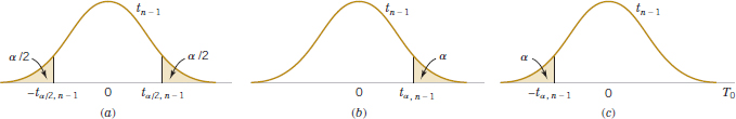
FIGURE 9-15 The distribution of T0 when H0: μ = μ0 is true with critical region for (a) H1:μ ≠ μ0, (b) H1:μ > μ0, and (c) H1:μ < μ0.
![]()
For the one-tailed tests, the location of the critical region is determined by the direction to which the inequality in the alternative hypothesis “points.” So, if the alternative is H1: μ > μ0, reject H0 if
![]()
and if the alternative is H1: μ < μ0, reject H0 if
![]()
Figure 9-15 provides the locations of these critical regions.
Summary for the One-Sample t-test
Testing Hypotheses on the Mean of a Normal Distribution, Variance Unknown Null hypothesis: H0: μ = μ0
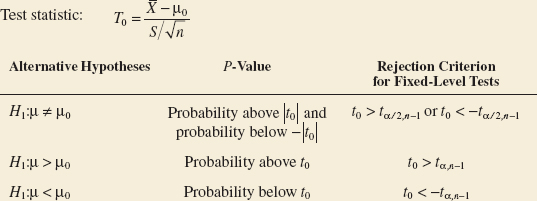
The calculations of the P-values and the locations of the critical regions for these situations are shown in Figs. 9-13 and 9-15, respectively.
Example 9-6 Golf Club Design The increased availability of light materials with high strength has revolutionized the design and manufacture of golf clubs, particularly drivers. Clubs with hollow heads and very thin faces can result in much longer tee shots, especially for players of modest skills. This is due partly to the “spring-like effect” that the thin face imparts to the ball. Firing a golf ball at the head of the club and measuring the ratio of the ball's outgoing velocity to the incoming velocity can quantify this spring-like effect. The ratio of velocities is called the coefficient of restitution of the club. An experiment was performed in which 15 drivers produced by a particular club maker were selected at random and their coefficients of restitution measured. In the experiment, the golf balls were fired from an air cannon so that the incoming velocity and spin rate of the ball could be precisely controlled. It is of interest to determine whether there is evidence (with α = 0.05) to support a claim that the mean coefficient of restitution exceeds 0.82. The observations follow:
![]()
The sample mean and sample standard deviation are ![]() = 0.83725 and s = 0.02456. The normal probability plot of the data in Fig. 9-16 supports the assumption that the coefficient of restitution is normally distributed. Because the experiment's objective is to demonstrate that the mean coefficient of restitution exceeds 0.82, a one-sided alternative hypothesis is appropriate.
= 0.83725 and s = 0.02456. The normal probability plot of the data in Fig. 9-16 supports the assumption that the coefficient of restitution is normally distributed. Because the experiment's objective is to demonstrate that the mean coefficient of restitution exceeds 0.82, a one-sided alternative hypothesis is appropriate.

FIGURE 9-16 Normal probability plot of the coefficient of restitution data from Example 9-6.
The solution using the seven-step procedure for hypothesis testing is as follows:
- Parameter of interest: The parameter of interest is the mean coefficient of restitution, μ.
- Null hypothesis: H0: μ = 0.82
- Alternative hypothesis: H1: μ > 0.82 We want to reject H0 if the mean coefficient of restitution exceeds 0.82.
- Test statistic: The test statistic is

- Reject H0 if: Reject H0 if the P-value is less than 0.05.
- Computations: Because = 0.83725, s = 0.02456, μ0 = 0.82, and n = 15, we have
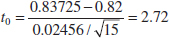
- Conclusions: From Appendix A Table II we find for a t distribution with 14 degrees of freedom that t0 = 2.72 falls between two values: 2.624, for which α = 0.01, and 2.977, for which α = 0.005. Because this is a one-tailed test, we know that the P-value is between those two values, that is, 0.005 < P < 0.01. Therefore, because P < 0.05, we reject H0 and conclude that the mean coefficient of restitution exceeds 0.82.
Practical Interpretation: There is strong evidence to conclude that the mean coefficient of restitution exceeds 0.82.
Normality and the t-Test
The development of the t-test assumes that the population from which the random sample is drawn is normal. This assumption is required to formally derive the t distribution as the reference distribution for the test statistic in Equation 9-26. Because it can be difficult to identify the form of a distribution based on a small sample, a logical question to ask is how important this assumption is. Studies have investigated this. Fortunately, studies have found that the t-test is relatively insensitive to the normality assumption. If the underlying population is reasonably symmetric and unimodal, the t-test will work satisfactorily. The exact significance level will not match the “advertised” level; for instance, the results may be significant at the 6% or 7% level instead of the 5% level. This is usually not a serious problem in practice. A normal probability plot of the sample data as illustrated for the golf club data in Figure 9-16 is usually a good way to verify the adequacy of the normality assumption. Only severe departures from normality that are evident in the plot should be a cause for concern.
Many software packages conduct the one-sample t-test. Typical computer output for Example 9-6 is shown in the following display:
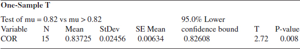
Notice that the software computes both the test statistic T0 and a 95% lower confidence bound for the coefficient of restitution. The reported P-value is 0.008. Because the 95% lower confidence bound exceeds 0.82, we would reject the hypothesis that H0: μ = 0.82 and conclude that the alternative hypothesis H1: μ > 0.82 is true.
9-3.2 TYPE II ERROR AND CHOICE OF SAMPLE SIZE
The type II error probability for the t-test depends on the distribution of the test statistic in Equation 9-26 when the null hypothesis H0: μ = μ0 is false. When the true value of the mean is μ = μ0 + δ, the distribution for T0 is called the noncentral t distribution with n − 1 degrees of freedom and noncentrality parameter δ![]() . Note that if δ = 0, the noncentral t distribution reduces to the usual central t distribution. Therefore, the type II error of the two-sided alternative (for example) would be
. Note that if δ = 0, the noncentral t distribution reduces to the usual central t distribution. Therefore, the type II error of the two-sided alternative (for example) would be
![]()
where ![]() denotes the noncentral t random variable. Finding the type II error probability β for the t-test involves finding the probability contained between two points of the noncentral t distribution. Because the noncentral t-random variable has a messy density function, this integration must be done numerically.
denotes the noncentral t random variable. Finding the type II error probability β for the t-test involves finding the probability contained between two points of the noncentral t distribution. Because the noncentral t-random variable has a messy density function, this integration must be done numerically.
Fortunately, this ugly task has already been done, and the results are summarized in a series of O.C. curves in Appendix Charts VIIe, VIIf, VIIg, and VIIh that plot β for the t-test against a parameter d for various sample sizes n. Curves are provided for two-sided alternatives on Charts VIIe and VIIf. The abscissa scale factor d on these charts is defined as
![]()
For the one-sided alternative μ > μ0 or μ < μ0, we use charts VIIg and VIIh with
![]()
We note that d depends on the unknown parameter σ2. We can avoid this difficulty in several ways. In some cases, we may use the results of a previous experiment or prior information to make a rough initial estimate of σ2. If we are interested in evaluating test performance after the data have been collected, we could use the sample variance s2 to estimate σ2. If there is no previous experience on which to draw in estimating σ2, we then define the difference in the mean d that we wish to detect relative to σ. For example, if we wish to detect a small difference in the mean, we might use a value of d = |δ|/σ ≤ 1 (for example), whereas if we are interested in detecting only moderately large differences in the mean, we might select d = |δ|/σ = 2 (for example). That is, the value of the ratio |δ|/σ is important in determining sample size, and if it is possible to specify the relative size of the difference in means that we are interested in detecting, then a proper value of d can usually be selected.
Example 9-7 Golf Club Design Sample Size Consider the golf club testing problem from Example 9-6. If the mean coefficient of restitution exceeds 0.82 by as much as 0.02, is the sample size n = 15 adequate to ensure that H0: μ = 0.82 will be rejected with probability at least 0.8?
To solve this problem, we will use the sample standard deviation s = 0.02456 to estimate σ. Then d = |δ|/σ = 0.02/0.02456 = 0.81. By referring to the operating characteristic curves in Appendix Chart VIIg (for α = 0.05) with d = 0.81 and n = 15, we find that β = 0.10, approximately. Thus, the probability of rejecting H0: μ = 0.82 if the true mean exceeds this by 0.02 is approximately 1 − β = 1 − 0.10 = 0.90, and we conclude that a sample size of n = 15 is adequate to provide the desired sensitivity.
Some software packages can also perform power and sample size computations for the one-sample t-test. Several calculations based on the golf club testing problem follow:
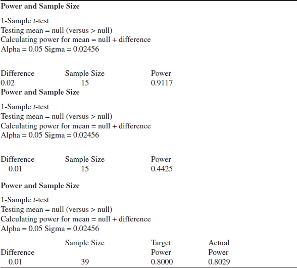
In the first portion of the computer output, the software reproduces the solution to Example 9-7, verifying that a sample size of n = 15 is adequate to give power of at least 0.8 if the mean coefficient of restitution exceeds 0.82 by at least 0.02. In the middle section of the output, we used the software to compute the power to detect the difference between μ and μ0 = 0.82 of 0.01. Notice that with n = 15, the power drops considerably to 0.4425. The final portion of the output is the sample size required for a power of at least 0.8 if the difference between μ and μ0 of interest is actually 0.01. A much larger n is required to detect this smaller difference.
![]() Problem available in WileyPLUS at instructor's discretion.
Problem available in WileyPLUS at instructor's discretion.
![]() Go Tutorial Tutoring problem available in WileyPLUS at instructor's discretion.
Go Tutorial Tutoring problem available in WileyPLUS at instructor's discretion.
9-52. ![]() A hypothesis will be used to test that a population mean equals 7 against the alternative that the population mean does not equal 7 with unknown variance. What are the critical values for the test statistic T0 for the following significance levels and sample sizes?
A hypothesis will be used to test that a population mean equals 7 against the alternative that the population mean does not equal 7 with unknown variance. What are the critical values for the test statistic T0 for the following significance levels and sample sizes?
(a) α = 0.01 and n = 20
(b) α = 0.05 and n = 12
(c) α = 0.10 and n = 15
9-53. A hypothesis will be used to test that a population mean equals 10 against the alternative that the population mean is greater than 10 with unknown variance. What is the critical value for the test statistic T0 for the following significance levels?
(a) α = 0.01 and n = 20
(b) α = 0.05 and n = 12
(c) α = 0.10 and n = 15
9-54. A hypothesis will be used to test that a population mean equals 5 against the alternative that the population mean is less than 5 with unknown variance. What is the critical value for the test statistic T0 for the following significance levels?
(a) α = 0.01 and n = 20
(b) α = 0.05 and n = 12
(c) α = 0.10 and n = 15
9-55. For the hypothesis test H0: μ = 7 against H1: μ ≠ 7 with variance unknown and n = 20, approximate the P-value for each of the following test statistics.
(a) t0 = 2.05
(b) t0 = −1.84
(c) t0 = 0.4
9-56. ![]() For the hypothesis test H0: μ = 10 against H1: μ > 10 with variance unknown and n = 15, approximate the P-value for each of the following test statistics.
For the hypothesis test H0: μ = 10 against H1: μ > 10 with variance unknown and n = 15, approximate the P-value for each of the following test statistics.
(a) t0 = 2.05
(b) t0 = −1.84
(c) t0 = 0.4
9-57. ![]() For the hypothesis test H0: μ = 5 against H1: μ < 5 with variance unknown and n = 12, approximate the P-value for each of the following test statistics.
For the hypothesis test H0: μ = 5 against H1: μ < 5 with variance unknown and n = 12, approximate the P-value for each of the following test statistics.
(a) t0 = 2.05
(b) t0 = −1.84
(c) t0 = 0.4
9-58. Consider the following computer output.

(a) Fill in the missing values. You may calculate bounds on the P-value. What conclusions would you draw?
(b) Is this a one-sided or a two-sided test?
(c) If the hypothesis had been H0: μ = 90 versus H1: μ > 90, would your conclusions change?
9-59. Consider the following computer output.

(a) How many degrees of freedom are there on the t-test statistic?
(b) Fill in the missing values. You may calculate bounds on the P-value. What conclusions would you draw?
(c) Is this a one-sided or a two-sided test?
(d) Construct a 95% two-sided CI on the mean.
(e) If the hypothesis had been H0: μ = 12 versus H1: μ > 12, would your conclusions change?
(f) If the hypothesis had been H0: μ = 11.5, versus H1: μ ≠ 11.5, would your conclusions change? Answer this question by using the CI computed in part (d).
9-60. Consider the following computer output.

(a) How many degrees of freedom are there on the t-test statistic?
(b) Fill in the missing quantities.
(c) At what level of significance can the null hypothesis be rejected?
(d) If the hypothesis had been H0: μ = 34 versus H1: μ > 34, would the P-value have been larger or smaller?
(e) If the hypothesis had been H0: μ = 34.5 versus H1: μ ≠ 34.5, would you have rejected the null hypothesis at the 0.05 level?
9-61. An article in Growth: A Journal Devoted to Problems of Normal and Abnormal Growth [“Comparison of Measured and Estimated Fat-Free Weight, Fat, Potassium and Nitrogen of Growing Guinea Pigs” (1982, Vol. 46(4), pp. 306–321)] reported the results of a study that measured the body weight (in grams) for guinea pigs at birth.
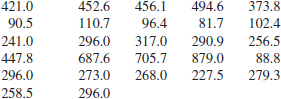
(a) Test the hypothesis that mean body weight is 300 grams. Use α = 0.05.
(b) What is the smallest level of significance at which you would be willing to reject the null hypothesis?
(c) Explain how you could answer the question in part (a) with a two-sided confidence interval on mean body weight.
9-62. An article in the ASCE Journal of Energy Engineering (1999, Vol. 125, pp. 59–75) describes a study of the thermal inertia properties of autoclaved aerated concrete used as a building material. Five samples of the material were tested in a structure, and the average interior temperatures (°C) reported were as follows: 23.01, 22.22, 22.04, 22.62, and 22.59.
(a) Test the hypotheses H0: μ = 22.5 versus H1: μ ≠ 22.5, using α = 0.05. Find the P-value.
(b) Check the assumption that interior temperature is normally distributed.
(c) Compute the power of the test if the true mean interior temperature is as high as 22.75.
(d) What sample size would be required to detect a true mean interior temperature as high as 22.75 if you wanted the power of the test to be at least 0.9?
(e) Explain how the question in part (a) could be answered by constructing a two-sided confidence interval on the mean interior temperature.
9-63. ![]() A 1992 article in the Journal of the American Medical Association (“A Critical Appraisal of 98.6 Degrees F, the Upper Limit of the Normal Body Temperature, and Other Legacies of Carl Reinhold August Wunderlich”) reported body temperature, gender, and heart rate for a number of subjects. The body temperatures for 25 female subjects follow: 97.8, 97.2, 97.4, 97.6, 97.8, 97.9, 98.0, 98.0, 98.0, 98.1, 98.2, 98.3, 98.3, 98.4, 98.4, 98.4, 98.5, 98.6, 98.6, 98.7, 98.8, 98.8, 98.9, 98.9, and 99.0.
A 1992 article in the Journal of the American Medical Association (“A Critical Appraisal of 98.6 Degrees F, the Upper Limit of the Normal Body Temperature, and Other Legacies of Carl Reinhold August Wunderlich”) reported body temperature, gender, and heart rate for a number of subjects. The body temperatures for 25 female subjects follow: 97.8, 97.2, 97.4, 97.6, 97.8, 97.9, 98.0, 98.0, 98.0, 98.1, 98.2, 98.3, 98.3, 98.4, 98.4, 98.4, 98.5, 98.6, 98.6, 98.7, 98.8, 98.8, 98.9, 98.9, and 99.0.
(a) Test the hypothesis H0: μ = 98.6 versus H1: μ ≠ 98.6, using α = 0.05. Find the P-value.
(b) Check the assumption that female body temperature is normally distributed.
(c) Compute the power of the test if the true mean female body temperature is as low as 98.0.
(d) What sample size would be required to detect a true mean female body temperature as low as 98.2 if you wanted the power of the test to be at least 0.9?
(e) Explain how the question in part (a) could be answered by constructing a two-sided confidence interval on the mean female body temperature.
9-64. ![]() Cloud seeding has been studied for many decades as a weather modification procedure (for an interesting study of this subject, see the article in Technometrics, “A Bayesian Analysis of a Multiplicative Treatment Effect in Weather Modification,” Vol. 17, pp. 161–166). The rainfall in acre-feet from 20 clouds that were selected at random and seeded with silver nitrate follows: 18.0, 30.7, 19.8, 27.1, 22.3, 18.8, 31.8, 23.4, 21.2, 27.9, 31.9, 27.1, 25.0, 24.7, 26.9, 21.8, 29.2, 34.8, 26.7, and 31.6.
Cloud seeding has been studied for many decades as a weather modification procedure (for an interesting study of this subject, see the article in Technometrics, “A Bayesian Analysis of a Multiplicative Treatment Effect in Weather Modification,” Vol. 17, pp. 161–166). The rainfall in acre-feet from 20 clouds that were selected at random and seeded with silver nitrate follows: 18.0, 30.7, 19.8, 27.1, 22.3, 18.8, 31.8, 23.4, 21.2, 27.9, 31.9, 27.1, 25.0, 24.7, 26.9, 21.8, 29.2, 34.8, 26.7, and 31.6.
(a) Can you support a claim that mean rainfall from seeded clouds exceeds 25 acre-feet? Use α = 0.01. Find the P-value.
(b) Check that rainfall is normally distributed.
(c) Compute the power of the test if the true mean rainfall is 27 acre-feet.
(d) What sample size would be required to detect a true mean rainfall of 27.5 acre-feet if you wanted the power of the test to be at least 0.9?
(e) Explain how the question in part (a) could be answered by constructing a one-sided confidence bound on the mean diameter.
9-65. ![]() The sodium content of twenty 300-gram boxes of organic cornflakes was determined. The data (in milligrams) are as follows: 131.15, 130.69, 130.91, 129.54, 129.64, 128.77, 130.72, 128.33, 128.24, 129.65, 130.14, 129.29, 128.71, 129.00, 129.39, 130.42, 129.53, 130.12, 129.78, 130.92.
The sodium content of twenty 300-gram boxes of organic cornflakes was determined. The data (in milligrams) are as follows: 131.15, 130.69, 130.91, 129.54, 129.64, 128.77, 130.72, 128.33, 128.24, 129.65, 130.14, 129.29, 128.71, 129.00, 129.39, 130.42, 129.53, 130.12, 129.78, 130.92.
(a) Can you support a claim that mean sodium content of this brand of cornflakes differs from 130 milligrams? Use α = 0.05. Find the P-value.
(b) Check that sodium content is normally distributed.
(c) Compute the power of the test if the true mean sodium content is 130.5 milligrams.
(d) What sample size would be required to detect a true mean sodium content of 130.1 milligrams if you wanted the power of the test to be at least 0.75?
(e) Explain how the question in part (a) could be answered by constructing a two-sided confidence interval on the mean sodium content.
9-66. Consider the baseball coefficient of restitution data first presented in Exercise 8-103.
(a) Do the data support the claim that the mean coefficient of restitution of baseballs exceeds 0.635? Use α = 0.05. Find the P-value.
(b) Check the normality assumption.
(c) Compute the power of the test if the true mean coefficient of restitution is as high as 0.64.
(d) What sample size would be required to detect a true mean coefficient of restitution as high as 0.64 if you wanted the power of the test to be at least 0.75?
(e) Explain how the question in part (a) could be answered with a confidence interval.
9-67. Consider the dissolved oxygen concentration at TVA dams first presented in Exercise 8-105.
(a) Test the hypothesis H0: μ = 4 versus H1: μ ≠ 4. Use α = 0.01. Find the P-value.
(b) Check the normality assumption.
(c) Compute the power of the test if the true mean dissolved oxygen concentration is as low as 3.
(d) What sample size would be required to detect a true mean dissolved oxygen concentration as low as 2.5 if you wanted the power of the test to be at least 0.9?
(e) Explain how the question in part (a) could be answered with a confidence interval.
9-68. ![]() Reconsider the data from Medicine and Science in Sports and Exercise described in Exercise 8-32. The sample size was seven and the sample mean and sample standard deviation were 315 watts and 16 watts, respectively.
Reconsider the data from Medicine and Science in Sports and Exercise described in Exercise 8-32. The sample size was seven and the sample mean and sample standard deviation were 315 watts and 16 watts, respectively.
(a) Is there evidence that leg strength exceeds 300 watts at significance level 0.05? Find the P-value.
(b) Compute the power of the test if the true strength is 305 watts.
(c) What sample size would be required to detect a true mean of 305 watts if the power of the test should be at least 0.90?
(d) Explain how the question in part (a) could be answered with a confidence interval.
9-69. Reconsider the tire testing experiment described in Exercise 8-29.
(a) The engineer would like to demonstrate that the mean life of this new tire is in excess of 60,000 kilometers. Formulate and test appropriate hypotheses, and draw conclusions using α = 0.05.
(b) Suppose that if the mean life is as long as 61,000 kilometers, the engineer would like to detect this difference with probability at least 0.90. Was the sample size n = 16 used in part (a) adequate?
9-70. Reconsider the Izod impact test on PVC pipe described in Exercise 8-30. Suppose that you want to use the data from this experiment to support a claim that the mean impact strength exceeds the ASTM standard (one foot-pound per inch). Formulate and test the appropriate hypotheses using α = 0.05.
9-71. ![]() Reconsider the television tube brightness experiment in Exercise 8-37. Suppose that the design engineer claims that this tube will require at least 300 microamps of current to produce the desired brightness level. Formulate and test an appropriate hypothesis to confirm this claim using α = 0.05. Find the P-value for this test. State any necessary assumptions about the underlying distribution of the data.
Reconsider the television tube brightness experiment in Exercise 8-37. Suppose that the design engineer claims that this tube will require at least 300 microamps of current to produce the desired brightness level. Formulate and test an appropriate hypothesis to confirm this claim using α = 0.05. Find the P-value for this test. State any necessary assumptions about the underlying distribution of the data.
9-72. Exercise 6-38 gave data on the heights of female engineering students at ASU.
(a) Can you support a claim that the mean height of female engineering students at ASU is at least 65 inches? Use α = 0.05. Find the P-value.
(b) Check the normality assumption.
(c) Compute the power of the test if the true mean height is 68 inches.
(d) What sample size would be required to detect a true mean height of 66 inches if you wanted the power of the test to be at least 0.8?
9-73. Exercise 6-41 describes testing golf balls for an overall distance standard.
(a) Can you support a claim that mean distance achieved by this particular golf ball exceeds 280 yards? Use α = 0.05. Find the P-value.
(b) Check the normality assumption.
(c) Compute the power of the test if the true mean distance is 290 yards.
(d) What sample size would be required to detect a true mean distance of 290 yards if you wanted the power of the test to be at least 0.8?
9-74. Exercise 6-40 presented data on the concentration of suspended solids in lake water.
(a) Test the hypothesis H0: μ = 55 versus H1: μ ≠ 55; use α = 0.05. Find the P-value.
(b) Check the normality assumption.
(c) Compute the power of the test if the true mean concentration is as low as 50.
(d) What sample size would be required to detect a true mean concentration as low as 50 if you wanted the power of the test to be at least 0.9?
9-75. Human oral normal body temperature is believed to be 98.6° F, but there is evidence that it actually should be 98.2° F [Mackowiak, Wasserman, Steven and Levine, JAMA (1992, Vol. 268(12), pp. 1578–1580)]. From a sample of 52 healthy adults, the mean oral temperature was 98.285 with a standard deviation of 0.625 degrees.
(a) What are the null and alternative hypotheses?
(b) Test the null hypothesis at α = 0.05.
(c) How does a 95% confidence interval answer the same question?
9-76. In a little over a month, from June 5, 1879, to July 2, 1879, Albert Michelson measured the velocity of light in air 100 times (Stigler, Annals of Statistics, 1977). Today we know that the true value is 299,734.5 km/sec. Michelson's data have a mean of 299,852.4 km/sec with a standard deviation of 79.01.
(a) Find a two-sided 95% confidence interval for the true mean (the true value of the speed of light).
(b) What does the confidence interval say about the accuracy of Michelson's measurements?
9-4 Tests on the Variance and Standard Deviation of a Normal Distribution
Sometimes hypothesis tests on the population variance or standard deviation are needed. When the population is modeled by a normal distribution, the tests and intervals described in this section are applicable.
9-4.1 HYPOTHESIS TESTS ON THE VARIANCE
Suppose that we wish to test the hypothesis that the variance of a normal population σ2 equals a specified value, say ![]() , or equivalently, that the standard deviation σ is equal to σ0. Let X1, X2,..., Xn be a random sample of n observations from this population. To test
, or equivalently, that the standard deviation σ is equal to σ0. Let X1, X2,..., Xn be a random sample of n observations from this population. To test
![]()
we will use the test statistic:
Test Statistic
![]()
If the null hypothesis H0: σ2 = ![]() is true, the test statistic
is true, the test statistic ![]() defined in Equation 9-35 follows the chi-square distribution with n − 1 degrees of freedom. This is the reference distribution for this test procedure. To perform a fixed significance level test, we would take a random sample from the population of interest, calculate
defined in Equation 9-35 follows the chi-square distribution with n − 1 degrees of freedom. This is the reference distribution for this test procedure. To perform a fixed significance level test, we would take a random sample from the population of interest, calculate ![]() , the value of the test statistic
, the value of the test statistic ![]() , and the null hypothesis H0:σ2 =
, and the null hypothesis H0:σ2 = ![]() would be rejected if
would be rejected if
![]()
where ![]() and
and ![]() are the upper and lower 100α/2 percentage points of the chi-square distribution with n − 1 degrees of freedom, respectively. Figure 9-17(a) shows the critical region.
are the upper and lower 100α/2 percentage points of the chi-square distribution with n − 1 degrees of freedom, respectively. Figure 9-17(a) shows the critical region.
The same test statistic is used for one-sided alternative hypotheses. For the one-sided hypotheses
![]()
we would reject H0 if ![]() , whereas for the other one-sided hypotheses
, whereas for the other one-sided hypotheses
![]()
we would reject H0 if ![]() . The one-sided critical regions are shown in Fig. 9-17(b) and (c).
. The one-sided critical regions are shown in Fig. 9-17(b) and (c).
Tests on the Variance of a Normal Distribution
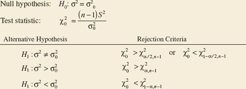
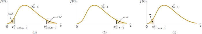
FIGURE 9-17 Reference distribution for the test of H0: σ2 = ![]() with critical region values for (a) H1: σ2 ≠
with critical region values for (a) H1: σ2 ≠ ![]() . (b) H1: σ2 >
. (b) H1: σ2 > ![]() . (c) H1: σ2 <
. (c) H1: σ2 < ![]() .
.
Example 9-8 Automated Filling An automated filling machine is used to fill bottles with liquid detergent. A random sample of 20 bottles results in a sample variance of fill volume of s2 = 0.0153 (fluidounces)2. If the variance of fill volume exceeds 0.01 (fluid ounces)2, an unacceptable proportion of bottles will be underfilled or overfilled. Is there evidence in the sample data to suggest that the manufacturer has a problem with underfilled or overfilled bottles? Use α = 0.05, and assume that fill volume has a normal distribution.
Using the seven-step procedure results in the following:
- Parameter of interest: The parameter of interest is the population variance σ2.
- Null hypothesis: H0: σ2 = 0.01
- Alternative hypothesis: H0: σ2 > 0.01
- Test statistic: The test statistic is

- Reject H0 if: Use α = 0.05, and reject H0 if
 = 30.14
 - Computations:
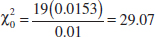
- Conclusions: Because
 = 29.07 <
  = 30.14, we conclude that there is no strong evidence that the variance of fill volume exceeds 0.01 fluid ounces2. So there is no strong evidence of a problem with incorrectly filled bottles.
We can also use the P-value approach. Using Appendix Table III, it is easy to place bounds on the P-value of a chi-square test. From inspection of the table, we find that ![]() = 27.20 and
= 27.20 and ![]() = 30.14. Because 27.20 < 29.07 < 30.14, we conclude that the P-value for the test in Example 9-8 is in the interval 0.05 < P-value < 0.10.
= 30.14. Because 27.20 < 29.07 < 30.14, we conclude that the P-value for the test in Example 9-8 is in the interval 0.05 < P-value < 0.10.
The P-value for a lower-tailed test would be found as the area (probability) in the lower tail of the chi-square distribution to the left of (or below) the computed value of the test statistic ![]() . For the two-sided alternative, find the tail area associated with the computed value of the test statistic and double it to obtain the P-value.
. For the two-sided alternative, find the tail area associated with the computed value of the test statistic and double it to obtain the P-value.
Some software packages perform the test on a variance of a normal distribution described in this section. Typical computer output for Example 9-8 is as follows:

Recall that we said that t-test is relatively robust to the assumption that we are sampling from a normal distribution. The same is not true for the chi-square test on variance. Even moderate departures from normality can result in the test statistic in Equation 9-35 having a distribution that is very different from chi-square.
9-4.2 TYPE II ERROR AND CHOICE OF SAMPLE SIZE
Operating characteristic curves for the chi-square tests in Section 9-4.1 are in Appendix Charts VIi through VIn for α = 0.05 and α = 0.01. For the two-sided alternative hypothesis of Equation 9-34, Charts VIIi and VIIj plot β against an abscissa parameter
![]()
for various sample sizes n, where σ denotes the true value of the standard deviation. Charts VIk and VIl are for the one-sided alternative H1: σ2 > ![]() , and Charts VIIm and VIIn are for the other one-sided alternative H1: σ2 <
, and Charts VIIm and VIIn are for the other one-sided alternative H1: σ2 < ![]() . In using these charts, we think of σ as the value of the standard deviation that we want to detect.
. In using these charts, we think of σ as the value of the standard deviation that we want to detect.
These curves can be used to evaluate the β-error (or power) associated with a particular test. Alternatively, they can be used to design a test—that is, to determine what sample size is necessary to detect a particular value of σ that differs from the hypothesized value σ0.
Example 9-9 Automated Filling Sample Size Consider the bottle-filling problem from Example 9-8. If the variance of the filling process exceeds 0.01 (fluid ounces)2, too many bottles will be underfilled. Thus, the hypothesized value of the standard deviation is σ0 = 0.10. Suppose that if the true standard deviation of the filling process exceeds this value by 25%, we would like to detect this with probability at least 0.8. Is the sample size of n = 20 adequate?
To solve this problem, note that we require
![]()
This is the abscissa parameter for Chart VIIk. From this chart, with n = 20 and λ = 1.25, we find that β ![]() 0.6. Therefore, there is only about a 40% chance that the null hypothesis will be rejected if the true standard deviation is really as large as σ = 0.125 fluid ounce.
0.6. Therefore, there is only about a 40% chance that the null hypothesis will be rejected if the true standard deviation is really as large as σ = 0.125 fluid ounce.
To reduce the β-error, a larger sample size must be used. From the operating characteristic curve with β = 0.20 and λ = 1.25, we find that n = 75, approximately. Thus, if we want the test to perform as required, the sample size must be at least 75 bottles.
Exercises FOR SECTION 9-4
![]() Problem available in WileyPLUS at instructor's discretion.
Problem available in WileyPLUS at instructor's discretion.
![]() Go Tutorial Tutoring problem available in WileyPLUS at instructor's discretion.
Go Tutorial Tutoring problem available in WileyPLUS at instructor's discretion.
9-77. ![]() Consider the test of H0:σ2 = 7 against H1:σ2 ≠ 7. What are the critical values for the test statistic
Consider the test of H0:σ2 = 7 against H1:σ2 ≠ 7. What are the critical values for the test statistic ![]() for the following significance levels and sample sizes?
for the following significance levels and sample sizes?
(a) α = 0.01 and n = 20
(b) α = 0.05 and n = 12
(c) α = 0.10 and n = 15
9-78. ![]() Consider the test of H0: σ2 = 10 against H1: σ2 > 10. What are the critical values for the test statistic
Consider the test of H0: σ2 = 10 against H1: σ2 > 10. What are the critical values for the test statistic ![]() for the following significance levels and sample sizes?
for the following significance levels and sample sizes?
(a) α = 0.01 and n = 20
(b) α = 0.05 and n = 12
(c) α = 0.10 and n = 15
9-79. Consider the test of H0: σ2 = 5 against H1: σ2 < 5. What are the critical values for the test statistic ![]() for the following significance levels and sample sizes?
for the following significance levels and sample sizes?
(a) α = 0.01 and n = 20
(b) α = 0.05 and n = 12
(c) α = 0.10 and n = 15
9-80. Consider the hypothesis test of H0:σ2 = 7 against H1:σ2 ≠ 7. Approximate the P-value for each of the following test statistics.
(a) ![]() = 25.2 and n = 20
= 25.2 and n = 20
(b) ![]() = 15.2 and n = 12
= 15.2 and n = 12
(c) ![]() = 23.0 and n = 15
= 23.0 and n = 15
9-81. ![]() Consider the test of H0: σ2 = 5 against H1: σ2 < 5. Approximate the P-value for each of the following test statistics.
Consider the test of H0: σ2 = 5 against H1: σ2 < 5. Approximate the P-value for each of the following test statistics.
(a) ![]() = 25.2 and n = 20
= 25.2 and n = 20
(b) ![]() = 15.2 and n = 12
= 15.2 and n = 12
(c) ![]() = 4.2 and n = 15
= 4.2 and n = 15
9-82. ![]() Consider the hypothesis test of H0:σ2 = 10 against H1:σ2 > 10. Approximate the P-value for each of the following test statistics.
Consider the hypothesis test of H0:σ2 = 10 against H1:σ2 > 10. Approximate the P-value for each of the following test statistics.
(a) ![]() = 25.2 and n = 20
= 25.2 and n = 20
(b) ![]() = 15.2 and n = 12
= 15.2 and n = 12
(c) ![]() = 4.2 and n = 15
= 4.2 and n = 15
9-83. The data from Medicine and Science in Sports and Exercise described in Exercise 8-53 considered ice hockey player performance after electrostimulation training. In summary, there were 17 players, and the sample standard deviation of performance was 0.09 seconds.
(a) Is there strong evidence to conclude that the standard deviation of performance time exceeds the historical value of 0.75 seconds? Use α = 0.05. Find the P-value for this test.
(b) Discuss how part (a) could be answered by constructing a 95% one-sided confidence interval for σ.
9-84. The data from Technometrics described in Exercise 8-56 considered the variability in repeated measurements of the weight of a sheet of paper. In summary, the sample standard deviation from 15 measurements was 0.0083 grams.
(a) Does the measurement standard deviation differ from 0.01 grams at α = 0.05? Find the P-value for this test.
(b) Discuss how part (a) could be answered by constructing a confidence interval for σ.
9-85. ![]() Reconsider the percentage of titanium in an alloy used in aerospace castings from Exercise 8-52. Recall that s = 0.37 and n = 51.
Reconsider the percentage of titanium in an alloy used in aerospace castings from Exercise 8-52. Recall that s = 0.37 and n = 51.
(a) Test the hypothesis H0: σ = 0.25 versus H1: σ ≠ 0.25 using α = 0.05. State any necessary assumptions about the underlying distribution of the data. Find the P-value.
(b) Explain how you could answer the question in part (a) by constructing a 95% two-sided confidence interval for σ.
9-86. Data from an Izod impact test was described in Exercise 8-30. The sample standard deviation was 0.25 and n = 20 specimens were tested.
(a) Test the hypothesis that σ = 0.10 against an alternative specifying that σ ≠ 0.10, using α = 0.01, and draw a conclusion. State any necessary assumptions about the underlying distribution of the data.
(b) What is the P-value for this test?
(c) Could the question in part (a) have been answered by constructing a 99% two-sided confidence interval for σ2?
9-87. ![]() Data for tire life was described in Exercise 8-29. The sample standard deviation was 3645.94 kilometers and n = 16.
Data for tire life was described in Exercise 8-29. The sample standard deviation was 3645.94 kilometers and n = 16.
(a) Can you conclude, using α = 0.05, that the standard deviation of tire life is less than 4000 kilometers? State any necessary assumptions about the underlying distribution of the data. Find the P-value for this test.
(b) Explain how you could answer the question in part (a) by constructing a 95% one-sided confidence interval for σ.
9-88. ![]() If the standard deviation of hole diameter exceeds 0.01 millimeters, there is an unacceptably high probability that the rivet will not fit. Suppose that n = 15 and s = 0.008 millimeter.
If the standard deviation of hole diameter exceeds 0.01 millimeters, there is an unacceptably high probability that the rivet will not fit. Suppose that n = 15 and s = 0.008 millimeter.
(a) Is there strong evidence to indicate that the standard deviation of hole diameter exceeds 0.01 millimeter? Use α = 0.01. State any necessary assumptions about the underlying distribution of the data. Find the P-value for this test.
(b) Suppose that the actual standard deviation of hole diameter exceeds the hypothesized value by 50%. What is the probability that this difference will be detected by the test described in part (a)?
(c) If σ is really as large as 0.0125 millimeters, what sample size will be required to detect this with power of at least 0.8?
9-89. Recall the sugar content of the syrup in canned peaches from Exercise 8-51. Suppose that the variance is thought to be σ2 = 18 (milligrams)2. Recall that a random sample of n = 10 cans yields a sample standard deviation of s = 4.8 milligrams.
(a) Test the hypothesis H0: σ2 = 18 versus H1: σ2 ≠ 18 using α = 0.05. Find the P-value for this test.
(b) Suppose that the actual standard deviation is twice as large as the hypothesized value. What is the probability that this difference will be detected by the test described in part (a)?
(c) Suppose that the true variance is σ2 = 40. How large a sample would be required to detect this difference with probability at least 0.90?
9-5 Tests on a Population Proportion
It is often necessary to test hypotheses on a population proportion. For example, suppose that a random sample of size n has been taken from a large (possibly infinite) population and that X(≤ n) observations in this sample belong to a class of interest. Then ![]() = X/n is a point estimator of the proportion of the population p that belongs to this class. Note that n and p are the parameters of a binomial distribution. Furthermore, from Chapter 7, we know that the sampling distribution of
= X/n is a point estimator of the proportion of the population p that belongs to this class. Note that n and p are the parameters of a binomial distribution. Furthermore, from Chapter 7, we know that the sampling distribution of ![]() is approximately normal with mean p and variance p(1 − p)/n if p is not too close to either 0 or 1 and if n is relatively large. Typically, to apply this approximation we require that np and n(1 − p) be greater than or equal to 5. We will give a large-sample test that use the normal approximation to the binomial distribution.
is approximately normal with mean p and variance p(1 − p)/n if p is not too close to either 0 or 1 and if n is relatively large. Typically, to apply this approximation we require that np and n(1 − p) be greater than or equal to 5. We will give a large-sample test that use the normal approximation to the binomial distribution.
9-5.1 LARGE-SAMPLE TESTS ON A PROPORTION
Many engineering problems concern a random variable that follows the binomial distribution. For example, consider a production process that manufactures items that are classified as either acceptable or defective. Modelling the occurrence of defectives with the binomial distribution is usually reasonable when the binomial parameter p represents the proportion of defective items produced. Consequently, many engineering decision problems involve hypothesis testing about p.
![]()
An approximate test based on the normal approximation to the binomial will be given. As noted earlier, this approximate procedure will be valid as long as p is not extremely close to 0 or 1, and if the sample size is relatively large. Let X be the number of observations in a random sample of size n that belongs to the class associated with p. Then if the null hypothesis H0:p = p0 is true, we have X ~ N[np0, np0(1 − p0)], approximately. To test H0: p = p0, calculate the test statistic
Test Statistic
![]()
and determine the P-value. Because the test statistic follows a standard normal distribution if H0 is true, the P-value is calculated exactly like the P-value for the z-tests in Section 9-2. So for the two-sided alternative hypothesis, the P-value is the sum of the probability in the standard normal distribution above |z0| and the probability below the negative value −|z0|, or
![]()
For the one-sided alternative hypothesis H0:p > p0, the P-value is the probability above z0, or
![]()
and for the one-sided alternative hypothesis H0: p < p0, the P-value is the probability below z0, or
![]()
We can also perform a fixed-significance-level test. For the two-sided alternative hypothesis, we would reject H0: p ≠ p0 if
![]()
Critical regions for the one-sided alternative hypotheses would be constructed in the usual manner.
Summary of Approximate Tests on a Binomial Proportion
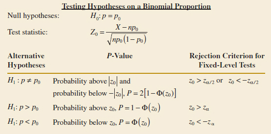
Example 9-10 Automobile Engine Controller A semiconductor manufacturer produces controllers used in automobile engine applications. The customer requires that the process fallout or fraction defective at a critical manufacturing step not exceed 0.05 and that the manufacturer demonstrate process capability at this level of quality using α = 0.05. The semiconductor manufacturer takes a random sample of 200 devices and finds that four of them are defective. Can the manufacturer demonstrate process capability for the customer?
We may solve this problem using the seven-step hypothesis-testing procedure as follows:
- Parameter of interest: The parameter of interest is the process fraction defective p.
- Null hypothesis: H0: p = 0.05
- Alternative hypothesis: H1: p < 0.05
This formulation of the problem will allow the manufacturer to make a strong claim about process capability if the null hypothesis H0: p = 0.05 is rejected.
- Test statistic: The test statistic is (from Equation 9-40):
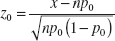
where x = 4, n = 200, and p0 = 0.05.
- Reject H0 if: Reject H0: p = 0.05 if the p-value is less than 0.05.
- Computation: The test statistic is
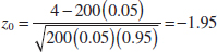
- Conclusions: Because z0 = −1.95, the P-value is Φ(−1.95) = 0.0256, so we reject H0 and conclude that the process fraction defective p is less than 0.05.
Practical Interpretation: We conclude that the process is capable.
Another form of the test statistic Z0 in Equation 9-40 is occasionally encountered. Note that if X is the number of observations in a random sample of size n that belongs to a class of interest, then ![]() = X/n is the sample proportion that belongs to that class. Now divide both numerator and denominator of Z0 in Equation 9-40 by n, giving
= X/n is the sample proportion that belongs to that class. Now divide both numerator and denominator of Z0 in Equation 9-40 by n, giving
![]()
This presents the test statistic in terms of the sample proportion instead of the number of items X in the sample that belongs to the class of interest.
Computer software packages can be used to perform the test on a binomial proportion. The following output shows typical results for Example 9-10.
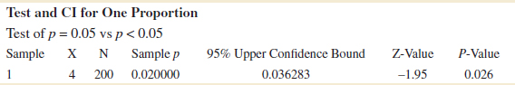
This output also shows a 95% one-sided upper-confidence bound on P. In Section 8-4, we showed how CIs on a binomial proportion are computed. This display shows the result of using the normal approximation for tests and CIs. When the sample size is small, this may be inappropriate.
Small Sample Tests on a Binomial Proportion
Tests on a proportion when the sample size n is small are based on the binomial distribution, not the normal approximation to the binomial. To illustrate, suppose that we wish to test H0: p < p0. Let X be the number of successes in the sample. The P-value for this test would be found from the lower tail of a binomial distribution with parameters n and p0. Specifically, the P-value would be the probability that a binomial random variable with parameters n and p0 is less than or equal to X. P-values for the upper-tailed one-sided test and the two-sided alternative are computed similarly.
Many software packages calculate the exact P-value for a binomial test. The following output contains the exact P-value results for Example 9-10.

The P-value is the same as that reported for the normal approximation because the sample size is fairly large. Notice that the CI is different from the one found using the normal approximation.
9-5.2 TYPE II ERROR AND CHOICE OF SAMPLE SIZE
It is possible to obtain closed-form equations for the approximate β-error for the tests in Section 9-5.1. Suppose that p is the true value of the population proportion. The approximate β-error for the two-sided alternative H1: p ≠ p0 is
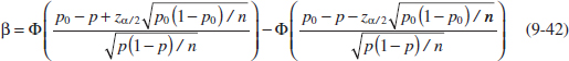
If the alternative is H1: p < p0,
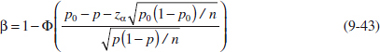
whereas if the alternative is H1: p > p0,

These equations can be solved to find the approximate sample size n that gives a test of level α that has a specified β risk. The sample size equations are
Approximate Sample Size for a Two-Sided Test on a Binomial Proportion
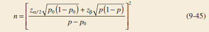
for a two-sided alternative and for a one-sided alternative:
Approximate Sample Size for a One-Sided Test on a Binomial Proportion
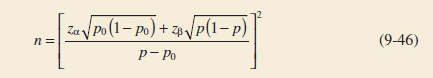
Example 9-11 Automobile Engine Controller Type II Error Consider the semiconductor manufacturer from Example 9-10. Suppose that its process fallout is really p = 0.03. What is the β-error for a test of process capability that uses n = 200 and α = 0.05?
The β-error can be computed using Equation 9-43 as follows:
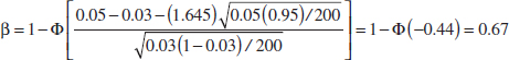
Thus, the probability is about 0.7 that the semiconductor manufacturer will fail to conclude that the process is capable if the true process fraction defective is p = 0.03 (3%). That is, the power of the test against this particular alternative is only about 0.3. This appears to be a large β-error (or small power), but the difference between p = 0.05 and p = 0.03 is fairly small, and the sample size n = 200 is not particularly large.
Suppose that the semiconductor manufacturer was willing to accept a β-error as large as 0.10 if the true value of the process fraction defective was p = 0.03. If the manufacturer continues to use α = 0.05, what sample size would be required?
The required sample size can be computed from Equation 9-46 as follows:
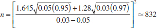
where we have used p = 0.03 in Equation 9-46.
Conclusion: Note that n = 832 is a very large sample size. However, we are trying to detect a fairly small deviation from the null value p0 = 0.05.
Some software packages also perform power and sample size calculations for the one-sample Z-test on a proportion. Typical computer output for the engine controllers tested in Example 9-10 follows.
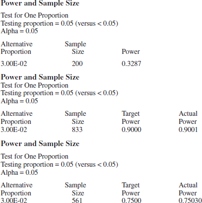
The first part of the output shows the power calculation based on the situation described in Example 9-11 where the true proportion is really 0.03. The computer power calculation agrees with the results from Equation 9-43 in Example 9-11. The second part of the output computes the sample size necessary for a power of 0.9 (β = 0.1) if p = 0.03. Again, the results agree closely with those obtained from Equation 9-46. The final portion of the display shows the sample size that would be required if p = 0.03 and the power requirement is relaxed to 0.75. Notice that the sample size of n = 561 is still quite large because the difference between p = 0.05 and p = 0.03 is fairly small.
![]() Problem available in WileyPLUS at instructor's discretion.
Problem available in WileyPLUS at instructor's discretion.
![]() Go Tutorial Tutoring problem available in WileyPLUS at instructor's discretion.
Go Tutorial Tutoring problem available in WileyPLUS at instructor's discretion.
9-90. Consider the following computer output
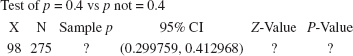
Using the normal approximation.
(a) Is this a one-sided or a two-sided test?
(b) Complete the missing items.
(c) The normal approximation was used in the problem. Was that appropriate?
9-91. Consider the following computer output

(a) Is this a one-sided or a two-sided test?
(b) Is this a test based on the normal approximation? Is that appropriate?
(c) Complete the missing items.
(d) Suppose that the alternative hypothesis was two-sided. What is the P-value for this situation?
9-92. ![]() Suppose that of 1000 customers surveyed, 850 are satisfied or very satisfied with a corporation's products and services.
Suppose that of 1000 customers surveyed, 850 are satisfied or very satisfied with a corporation's products and services.
(a) Test the hypothesis H0: p = 0.9 against H1: p ≠ 0.9 at α = 0.05. Find the P-value.
(b) Explain how the question in part (a) could be answered by constructing a 95% two-sided confidence interval for p.
9-93. ![]() Suppose that 500 parts are tested in manufacturing and 10 are rejected.
Suppose that 500 parts are tested in manufacturing and 10 are rejected.
(a) Test the hypothesis H0: p = 0.03 against H1: p < 0.03 at α = 0.05. Find the P-value.
(b) Explain how the question in part (a) could be answered by constructing a 95% one-sided confidence interval for p.
9-94. ![]() A random sample of 300 circuits generated 13 defectives.
A random sample of 300 circuits generated 13 defectives.
(a) Use the data to test H0: p = 0.05 versus H1: p ≠ 0.05. Use α = 0.05. Find the P-value for the test.
(b) Explain how the question in part (a) could be answered with a confidence interval.
9-95. An article in the British Medical Journal [“Comparison of Treatment of Renal Calculi by Operative Surgery, Percutaneous Nephrolithotomy, and Extra-Corporeal Shock Wave Lithotrips” (1986, Vol. 292, pp. 879–882)] repeated that percutaneous nephrolithotomy (PN) had a success rate in removing kidney stones of 289 of 350 patients. The traditional method was 78% effective.
(a) Is there evidence that the success rate for PN is greater than the historical success rate? Find the P-value.
(b) Explain how the question in part (a) could be answered with a confidence interval.
9-96. ![]() A manufacturer of interocular lenses will qualify a new grinding machine if there is evidence that the percentage of polished lenses that contain surface defects does not exceed 2%. A random sample of 250 lenses contains 6 defective lenses.
A manufacturer of interocular lenses will qualify a new grinding machine if there is evidence that the percentage of polished lenses that contain surface defects does not exceed 2%. A random sample of 250 lenses contains 6 defective lenses.
(a) Formulate and test an appropriate set of hypotheses to determine whether the machine can be qualified. Use α = 0.05. Find the P-value.
(b) Explain how the question in part (a) could be answered with a confidence interval.
9-97. ![]() A researcher claims that at least 10% of all football helmets have manufacturing flaws that could potentially cause injury to the wearer. A sample of 200 helmets revealed that 16 helmets contained such defects.
A researcher claims that at least 10% of all football helmets have manufacturing flaws that could potentially cause injury to the wearer. A sample of 200 helmets revealed that 16 helmets contained such defects.
(a) Does this finding support the researcher's claim? Use α = 0.01. Find the P-value.
(b) Explain how the question in part (a) could be answered with a confidence interval.
9-98. ![]() An article in Fortune (September 21, 1992) claimed that nearly one-half of all engineers continue academic studies beyond the B.S. degree, ultimately receiving either an M.S. or a Ph.D. degree. Data from an article in Engineering Horizons (Spring 1990) indicated that 117 of 484 new engineering graduates were planning graduate study.
An article in Fortune (September 21, 1992) claimed that nearly one-half of all engineers continue academic studies beyond the B.S. degree, ultimately receiving either an M.S. or a Ph.D. degree. Data from an article in Engineering Horizons (Spring 1990) indicated that 117 of 484 new engineering graduates were planning graduate study.
(a) Are the data from Engineering Horizons consistent with the claim reported by Fortune? Use α = 0.05 in reaching your conclusions. Find the P-value for this test.
(b) Discuss how you could have answered the question in part (a) by constructing a two-sided confidence interval on p.
9-99. ![]() The advertised claim for batteries for cell phones is set at 48 operating hours with proper charging procedures. A study of 5000 batteries is carried out and 15 stop operating prior to 48 hours. Do these experimental results support the claim that less than 0.2 percent of the company's batteries will fail during the advertised time period, with proper charging procedures? Use a hypothesis-testing procedure with α = 0.01.
The advertised claim for batteries for cell phones is set at 48 operating hours with proper charging procedures. A study of 5000 batteries is carried out and 15 stop operating prior to 48 hours. Do these experimental results support the claim that less than 0.2 percent of the company's batteries will fail during the advertised time period, with proper charging procedures? Use a hypothesis-testing procedure with α = 0.01.
9-100. ![]() A random sample of 500 registered voters in Phoenix is asked if they favor the use of oxygenated fuels year-round to reduce air pollution. If more than 315 voters respond positively, we will conclude that at least 60% of the voters favor the use of these fuels.
A random sample of 500 registered voters in Phoenix is asked if they favor the use of oxygenated fuels year-round to reduce air pollution. If more than 315 voters respond positively, we will conclude that at least 60% of the voters favor the use of these fuels.
(a) Find the probability of type I error if exactly 60% of the voters favor the use of these fuels.
(b) What is the type II error probability β if 75% of the voters favor this action?
9-101. In a random sample of 85 automobile engine crankshaft bearings, 10 have a surface finish roughness that exceeds the specifications. Do these data present strong evidence that the proportion of crankshaft bearings exhibiting excess surface roughness exceeds 0.10?
(a) State and test the appropriate hypotheses using α = 0.05.
(b) If it is really the situation that p = 0.15, how likely is it that the test procedure in part (a) will not reject the null hypothesis?
(c) If p = 0.15, how large would the sample size have to be for us to have a probability of correctly rejecting the null hypothesis of 0.9?
9-102. A computer manufacturer ships laptop computers with the batteries fully charged so that customers can begin to use their purchases right out of the box. In its last model, 85% of customers received fully charged batteries. To simulate arrivals, the company shipped 100 new model laptops to various company sites around the country. Of the 105 laptops shipped, 96 of them arrived reading 100% charged. Do the data provide evidence that this model's rate is at least as high as the previous model? Test the hypothesis at α = 0.05.
9-103. In a random sample of 500 handwritten zip code digits, 466 were read correctly by an optical character recognition (OCR) system operated by the U.S. Postal Service (USPS). USPS would like to know whether the rate is at least 90% correct. Do the data provide evidence that the rate is at least 90% at α = 0.05?
9-104. Construct a 90% confidence interval for the proportion of handwritten zip codes that were read correctly using the data provided in Exercise 9-103. Does this confidence interval support the claim that at least 90% of the zip codes can be correctly read?
9-105. Construct a 95% lower confidence interval for the proportion of patients with kidney stones successfully removed in Exercise 9-95. Does this confidence interval support the claim that at least 78% of procedures are successful?
9-6 Summary Table of Inference Procedures for a Single Sample
The table in the end papers of this book (inside back cover) presents a summary of all the single-sample inference procedures from Chapters 8 and 9. The table contains the null hypothesis statement, the test statistic, the various alternative hypotheses and the criteria for rejecting H0, and the formulas for constructing the 100(1 − α)% two-sided confidence interval. It would also be helpful to refer to the roadmap table in Chapter 8 that provides guidance to match the problem type to the information inside the back cover.
9-7 Testing for Goodness of Fit
The hypothesis-testing procedures that we have discussed in previous sections are designed for problems in which the population or probability distribution is known and the hypotheses involve the parameters of the distribution. Another kind of hypothesis is often encountered: We do not know the underlying distribution of the population, and we wish to test the hypothesis that a particular distribution will be satisfactory as a population model. For example, we might wish to test the hypothesis that the population is normal.
We have previously discussed a very useful graphical technique for this problem called probability plotting and illustrated how it was applied in the case of a normal distribution. In this section, we describe a formal goodness-of-fit test procedure based on the chi-square distribution.
The test procedure requires a random sample of size n from the population whose probability distribution is unknown. These n observations are arranged in a frequency histogram, having k bins or class intervals. Let Oi be the observed frequency in the ith class interval. From the hypothesized probability distribution, we compute the expected frequency in the ith class interval, denoted Ei. The test statistic is
Goodness-of-Fit Test Statistic

It can be shown that, if the population follows the hypothesized distribution, ![]() has, approximately, a chi-square distribution with k − p − 1 degrees of freedom, when p represents the number of parameters of the hypothesized distribution estimated by sample statistics. This approximation improves as n increases. We should reject the null hypothesis that the population is the hypothesized distribution if the test statistic is too large. Therefore, the P-value would be the probability under the chi-square distribution with k − p − 1 degrees of freedom above the computed value of the test statistic
has, approximately, a chi-square distribution with k − p − 1 degrees of freedom, when p represents the number of parameters of the hypothesized distribution estimated by sample statistics. This approximation improves as n increases. We should reject the null hypothesis that the population is the hypothesized distribution if the test statistic is too large. Therefore, the P-value would be the probability under the chi-square distribution with k − p − 1 degrees of freedom above the computed value of the test statistic ![]() or P = P
or P = P![]() . For a fixed-level test, we would reject the hypothesis that the distribution of the population is the hypothesized distribution if the calculated value of the test statistic
. For a fixed-level test, we would reject the hypothesis that the distribution of the population is the hypothesized distribution if the calculated value of the test statistic ![]() .
.
One point to be noted in the application of this test procedure concerns the magnitude of the expected frequencies. If these expected frequencies are too small, the test statistic ![]() will not reflect the departure of observed from expected but only the small magnitude of the expected frequencies. There is no general agreement regarding the minimum value of expected frequencies, but values of 3, 4, and 5 are widely used as minimal. Some writers suggest that an expected frequency could be as small as 1 or 2 so long as most of them exceed 5. Should an expected frequency be too small, it can be combined with the expected frequency in an adjacent class interval. The corresponding observed frequencies would then also be combined, and k would be reduced by 1. Class intervals are not required to be of equal width.
will not reflect the departure of observed from expected but only the small magnitude of the expected frequencies. There is no general agreement regarding the minimum value of expected frequencies, but values of 3, 4, and 5 are widely used as minimal. Some writers suggest that an expected frequency could be as small as 1 or 2 so long as most of them exceed 5. Should an expected frequency be too small, it can be combined with the expected frequency in an adjacent class interval. The corresponding observed frequencies would then also be combined, and k would be reduced by 1. Class intervals are not required to be of equal width.
We now give two examples of the test procedure.
Example 9-12 Printed Circuit Board Defects-Poisson Distribution The number of defects in printed circuit boards is hypothesized to follow a Poisson distribution. A random sample of n = 60 printed circuit boards has been collected, and the following number of defects observed.
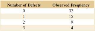
The mean of the assumed Poisson distribution in this example is unknown and must be estimated from the sample data. The estimate of the mean number of defects per board is the sample average, that is, (32·0 + 15·1 + 9·2 + 4·3)/60 = 0·75. From the Poisson distribution with parameter 0.75, we may compute pi, the theoretical, hypothesized probability associated with the ith class interval. Because each class interval corresponds to a particular number of defects, we may find the pi as follows:
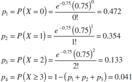
The expected frequencies are computed by multiplying the sample size n = 60 times the probabilities pi. That is, Ei = npi. The expected frequencies follow:
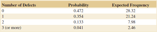
Because the expected frequency in the last cell is less than 3, we combine the last two cells:
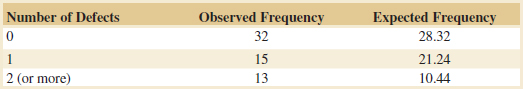
The seven-step hypothesis-testing procedure may now be applied, using α = 0.05, as follows:
- Parameter of interest: The variable of interest is the form of the distribution of defects in printed circuit boards.
- Null hypothesis: H0: The form of the distribution of defects is Poisson.
- Alternative hypothesis: H1: The form of the distribution of defects is not Poisson.
- Test statistic: The test statistic is
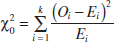
- Reject H0 if: Because the mean of the Poisson distribution was estimated, the preceding chi-square statistic will have k − p − 1 = 3 − 1 − 1 = 1 degree of freedom. Consider whether the P-value is less than 0.05.
- Computations:
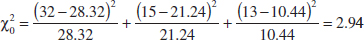
- Conclusions: We find from Appendix Table III that
 = 2.71 and
  = 3.84. Because
  = 2.94 lies between these values, we conclude that the P-value is between 0.05 and 0.10. Therefore, because the P-value exceeds 0.05, we are unable to reject the null hypothesis that the distribution of defects in printed circuit boards is Poisson. The exact P-value computed from software is 0.0864.
Example 9-13 Power Supply Distribution-Continuous Distribution A manufacturing engineer is testing a power supply used in a notebook computer and, using α = 0.05, wishes to determine whether output voltage is adequately described by a normal distribution. Sample estimates of the mean and standard deviation of ![]() = 5.04 V and s = 0.08 V are obtained from a random sample of n = 100 units.
= 5.04 V and s = 0.08 V are obtained from a random sample of n = 100 units.
A common practice in constructing the class intervals for the frequency distribution used in the chi-square goodness-of-fit test is to choose the cell boundaries so that the expected frequencies Ei = npi are equal for all cells. To use this method, we want to choose the cell boundaries a0, a1,..., ak for the k cells so that all the probabilities
![]()
are equal. Suppose that we decide to use k = 8 cells. For the standard normal distribution, the intervals that divide the scale into eight equally likely segments are (0, 0.32), (0.32, 0.675), (0.675, 1.15), (1.15, ∞), and their four “mirror image” intervals on the other side of zero. For each interval pi = 1/8 = 0.125, so the expected cell frequencies are Ei = npi = 100(0.125) = 12.5. The complete table of observed and expected frequencies is as follows:

The boundary of the first class interval is ![]() − 1.15s = 4.948. The second class interval is [
− 1.15s = 4.948. The second class interval is [![]() − 1.15s,
− 1.15s, ![]() − 0.675s] and so forth. We may apply the seven-step hypothesis-testing procedure to this problem.
− 0.675s] and so forth. We may apply the seven-step hypothesis-testing procedure to this problem.
- Parameter of interest: The variable of interest is the form of the distribution of power supply voltage.
- Null hypothesis: H0: The form of the distribution is normal.
- Alternative hypothesis: H1: The form of the distribution is nonnormal.
- Test statistic: The test statistic is
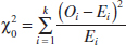
- Reject H0 if: Because two parameters in the normal distribution have been estimated, the preceding chi-square statistic will have k − p − 1 = 8 − 2 − 1 = 5 degrees of freedom. We will use a fixed significance level test with α = 0.05. Therefore, we will reject H0 if
 = 11.07.
 - Computations:
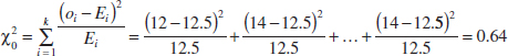
- Conclusions: Because
 = 0.64 <
  = 11.07, we are unable to reject H0, and no strong evidence indicates that output voltage is not normally distributed. The P-value for the chi-square statistic
  = 0.64 is P = 0.9861.
EXERCISES FOR SECTION 9-7
![]() Problem available in WileyPLUS at instructor's discretion.
Problem available in WileyPLUS at instructor's discretion.
![]() Go Tutorial Tutoring problem available in WileyPLUS at instructor's discretion.
Go Tutorial Tutoring problem available in WileyPLUS at instructor's discretion.
9-106. ![]() Consider the following frequency table of observations on the random variable X.
Consider the following frequency table of observations on the random variable X.
![]()
(a) Based on these 100 observations, is a Poisson distribution with a mean of 1.2 an appropriate model? Perform a goodness-of-fit procedure with α = 0.05.
(b) Calculate the P-value for this test.
9-107. ![]() Let X denote the number of flaws observed on a large coil of galvanized steel. Of 75 coils inspected, the following data were observed for the values of X:
Let X denote the number of flaws observed on a large coil of galvanized steel. Of 75 coils inspected, the following data were observed for the values of X:
![]()
(a) Does the assumption of the Poisson distribution seem appropriate as a probability model for these data? Use α = 0.01.
(b) Calculate the P-value for this test.
9-108. ![]() The number of calls arriving at a switchboard from noon to 1:00 P.M. during the business days Monday through Friday is monitored for six weeks (i.e., 30 days). Let X be defined as the number of calls during that one-hour period. The relative frequency of calls was recorded and reported as
The number of calls arriving at a switchboard from noon to 1:00 P.M. during the business days Monday through Friday is monitored for six weeks (i.e., 30 days). Let X be defined as the number of calls during that one-hour period. The relative frequency of calls was recorded and reported as

(a) Does the assumption of a Poisson distribution seem appropriate as a probability model for this data? Use α = 0.05.
(b) Calculate the P-value for this test.
9-109. ![]() Consider the following frequency table of observations on the random variable X:
Consider the following frequency table of observations on the random variable X:
![]()
(a) Based on these 50 observations, is a binomial distribution with n = 6 and p = 0.25 an appropriate model? Perform a goodness-of-fit procedure with α = 0.05.
(b) Calculate the P-value for this test.
9-110. ![]() Define X as the number of underfilled bottles from a filling operation in a carton of 24 bottles. Of 75 cartons inspected, the following observations on X are recorded:
Define X as the number of underfilled bottles from a filling operation in a carton of 24 bottles. Of 75 cartons inspected, the following observations on X are recorded:
![]()
(a) Based on these 75 observations, is a binomial distribution an appropriate model? Perform a goodness-of-fit procedure with α = 0.05.
(b) Calculate the P-value for this test.
9-111. A group of civil engineering students has tabulated the number of cars passing eastbound through the intersection of Mill and University Avenues. They obtained the data in the following table.
(a) Does the assumption of a Poisson distribution seem appropriate as a probability model for this process? Use α = 0.05.
(b) Calculate the P-value for this test.
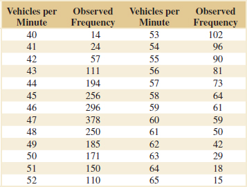
9-112. ![]() Reconsider Exercise 6-87. The data were the number of earthquakes per year of magnitude 7.0 and greater since 1900.
Reconsider Exercise 6-87. The data were the number of earthquakes per year of magnitude 7.0 and greater since 1900.
(a) Use computer software to summarize these data into a frequency distribution. Test the hypothesis that the number of earthquakes of magnitude 7.0 or greater each year follows a Poisson distribution at α = 0.05.
(b) Calculate the P-value for the test.
9-8 Contingency Table Tests
Many times the n elements of a sample from a population may be classified according to two different criteria. It is then of interest to know whether the two methods of classification are statistically independent; for example, we may consider the population of graduating engineers and may wish to determine whether starting salary is independent of academic disciplines. Assume that the first method of classification has r levels and that the second method has c levels. We will let Oij be the observed frequency for level i of the first classification method and level j of the second classification method. The data would, in general, appear as shown in Table 9-2. Such a table is usually called an r × c contingency table.
We are interested in testing the hypothesis that the row-and-column methods of classification are independent. If we reject this hypothesis, we conclude some interaction exists between the two criteria of classification. The exact test procedures are difficult to obtain, but an approximate test statistic is valid for large n. Let pij be the probability that a randomly selected element falls in the ijth cell given that the two classifications are independent. Then pij = uivj, where ui is the probability that a randomly selected element falls in row class i and vj is the probability that a randomly selected element falls in column class j. Now by assuming independence, the estimators of ui and vj are
![]()
![]() TABLE • 9-2 An r × c Contingency Table
TABLE • 9-2 An r × c Contingency Table
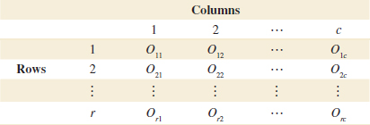
Therefore, the expected frequency of each cell is
![]()
Then, for large n, the statistic
![]()
has an approximate chi-square distribution with (r − 1)(c − 1) degrees of freedom if the null hypothesis is true. We should reject the null hypothesis if the value of the test statistic ![]() is too large. The P-value would be calculated as the probability beyond
is too large. The P-value would be calculated as the probability beyond ![]() on the
on the ![]() distribution, or P = P
distribution, or P = P![]() . For a fixed-level test, we would reject the hypothesis of independence if the observed value of the test statistic
. For a fixed-level test, we would reject the hypothesis of independence if the observed value of the test statistic ![]() exceeded
exceeded ![]() .
.
Example 9-14 Health Insurance Plan Preference A company has to choose among three health insurance plans. Management wishes to know whether the preference for plans is independent of job classification and wants to use α = 0.05. The opinions of a random sample of 500 employees are shown in Table 9-3.
![]() TABLE • 9-3 Observed Data for Example 9-14
TABLE • 9-3 Observed Data for Example 9-14

To find the expected frequencies, we must first compute ![]() 1 = (340/500) = 0.68,
1 = (340/500) = 0.68, ![]() 2 = (160/500) = 0.32,
2 = (160/500) = 0.32, ![]() 1 = (200/500) = 0.40,
1 = (200/500) = 0.40, ![]() 2 = (200/500) = 0.40, and
2 = (200/500) = 0.40, and ![]() 3 = (100/500) = 0.20. The expected frequencies may now be computed from Equation 9-49. For example, the expected number of salaried workers favoring health insurance plan 1 is
3 = (100/500) = 0.20. The expected frequencies may now be computed from Equation 9-49. For example, the expected number of salaried workers favoring health insurance plan 1 is
![]()
The expected frequencies are shown in Table 9-4.
![]() TABLE • 9-4 Expected Frequencies for Example 9-14
TABLE • 9-4 Expected Frequencies for Example 9-14

The seven-step hypothesis-testing procedure may now be applied to this problem.
- Parameter of interest: The variable of interest is employee preference among health insurance plans.
- Null hypothesis: H0: Preference is independent of salaried versus hourly job classification.
- Alternative hypothesis: H1: Preference is not independent of salaried versus hourly job classification.
- Test statistic: The test statistic is
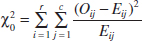
- Reject H0 if: We will use a fixed-significance level test with α = 0.05. Therefore, because r = 2 and c = 3, the degrees of freedom for chi-square are (r − 1)(c − 1) = (1)(2) = 2, and we would reject H0 if
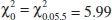 ·
· - Computations:

- Conclusions: Because
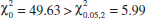 , we reject the hypothesis of independence and conclude that the preference for health insurance plans is not independent of job classification. The P-value for
  = 49.63 is P = 1.671 × 10⁻¹¹. (This value was computed by computer software.) Further analysis would be necessary to explore the nature of the association between these factors. It might be helpful to examine the table of observed minus expected frequencies.
Using the two-way contingency table to test independence between two variables of classification in a sample from a single population of interest is only one application of contingency table methods. Another common situation occurs when there are r populations of interest and each population is divided into the same c categories. A sample is then taken from the ith population, and the counts are entered in the appropriate columns of the ith row. In this situation, we want to investigate whether or not the proportions in the c categories are the same for all populations. The null hypothesis in this problem states that the populations are homogeneous with respect to the categories. For example, with only two categories, such as success and failure, defective and nondefective, and so on, the test for homogeneity is really a test of the equality of r binomial parameters. Calculation of expected frequencies, determination of degrees of freedom, and computation of the chi-square statistic for the test for homogeneity are identical to the test for independence.
EXERCISES FOR SECTION 9-8
![]() Problem available in WileyPLUS at instructor's discretion.
Problem available in WileyPLUS at instructor's discretion.
![]() Go Tutorial Tutoring problem available in WileyPLUS at instructor's discretion.
Go Tutorial Tutoring problem available in WileyPLUS at instructor's discretion.
9-113. The Hopkins Forest is a 2600-acre forest reserve located at the intersection of three states: New York, Vermont, and Massachusetts. Researchers monitor forest resources to study long-term ecological changes. They have conducted surveys of existing trees, shrubs, and herbs at various sites in the forest for nearly 100 years. Following are some data from surveys of three species of maple trees at the same location over three very different time periods.
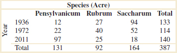
Does the species distribution seem to be independent of year? Test the hypothesis at α = 0.05. Find the P-value of the test statistic.
9-114. Did survival rate for passengers on the Titanic really depend on the type of ticket they had? Following are the data for the 2201 people on board listed by whether they survived and what type of ticket they had. Does survival appear to be independent of ticket class? (Test the hypothesis at α = 0.05.) What is the P-value of the test statistic?
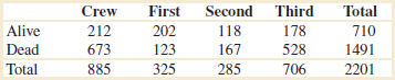
9-115. ![]() A company operates four machines in three shifts each day. From production records, the following data on the number of breakdowns are collected:
A company operates four machines in three shifts each day. From production records, the following data on the number of breakdowns are collected:

Test the hypothesis (using α = 0.05) that breakdowns are independent of the shift. Find the P-value for this test.
9-116. ![]() Patients in a hospital are classified as surgical or medical. A record is kept of the number of times patients require nursing service during the night and whether or not these patients are on Medicare. The data are presented here:
Patients in a hospital are classified as surgical or medical. A record is kept of the number of times patients require nursing service during the night and whether or not these patients are on Medicare. The data are presented here:

Test the hypothesis (using α = 0.01) that calls by surgical-medical patients are independent of whether the patients are receiving Medicare. Find the P-value for this test.
9-117. ![]() Grades in a statistics course and an operations research course taken simultaneously were as follows for a group of students.
Grades in a statistics course and an operations research course taken simultaneously were as follows for a group of students.

Are the grades in statistics and operations research related? Use α = 0.01 in reaching your conclusion. What is the P-value for this test?
9-118. ![]() An experiment with artillery shells yields the following data on the characteristics of lateral deflections and ranges. Would you conclude that deflection and range are independent? Use α = 0.05. What is the P-value for this test?
An experiment with artillery shells yields the following data on the characteristics of lateral deflections and ranges. Would you conclude that deflection and range are independent? Use α = 0.05. What is the P-value for this test?
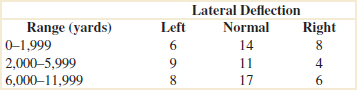
9-119. ![]() A study is being made of the failures of an electronic component. There are four types of failures possible and two mounting positions for the device. The following data have been taken:
A study is being made of the failures of an electronic component. There are four types of failures possible and two mounting positions for the device. The following data have been taken:

Would you conclude that the type of failure is independent of the mounting position? Use α = 0.01. Find the P-value for this test.
9-120. ![]() A random sample of students is asked their opinions on a proposed core curriculum change. The results are as follows.
A random sample of students is asked their opinions on a proposed core curriculum change. The results are as follows.

Test the hypothesis that opinion on the change is independent of class standing. Use α = 0.05. What is the P-value for this test?
9-121. ![]() An article in the British Medical Journal [“Comparison of Treatment of Renal Calculi by Operative Surgery, Percutaneous Nephrolithotomy, and Extracorporeal Shock Wave Lithotripsy” (1986, Vol. 292, pp. 879–882)] reported that percutaneous nephrolithotomy (PN) had a success rate in removing kidney stones of 289 out of 350 (83%) patients. However, when the stone diameter was considered, the results looked different. For stones of <2cm, 87% (234/270) of cases were successful. For stones of ≥2cm, a success rate of 69% (55/80) was observed for PN.
An article in the British Medical Journal [“Comparison of Treatment of Renal Calculi by Operative Surgery, Percutaneous Nephrolithotomy, and Extracorporeal Shock Wave Lithotripsy” (1986, Vol. 292, pp. 879–882)] reported that percutaneous nephrolithotomy (PN) had a success rate in removing kidney stones of 289 out of 350 (83%) patients. However, when the stone diameter was considered, the results looked different. For stones of <2cm, 87% (234/270) of cases were successful. For stones of ≥2cm, a success rate of 69% (55/80) was observed for PN.
(a) Are the successes and size of stones independent? Use α = 0.05.
(b) Find the P-value for this test.
9-9 Nonparametric Procedures
Most of the hypothesis-testing and confidence interval procedures discussed previously are based on the assumption that we are working with random samples from normal populations. Traditionally, we have called these procedures parametric methods because they are based on a particular parametric family of distributions—in this case, the normal. Alternately, sometimes we say that these procedures are not distribution free because they depend on the assumption of normality. Fortunately, most of these procedures are relatively insensitive to moderate departures from normality. In general, the t- and F-tests and the t-confidence intervals will have actual levels of significance or confidence levels that differ from the nominal or advertised levels chosen by the experimenter, although the difference in the actual and advertised levels is usually fairly small when the underlying population is not too different from the normal.
In this section, we describe procedures called nonparametric and distribution-free methods, and we usually make no assumptions about the distribution of the underlying population other than that it is continuous. These procedures have an accurate level of significance α or confidence level 100(1 − α)% for many different types of distributions. These procedures have some appeal. One of their advantages is that the data need not be quantitative but can be categorical (such as yes or no, defective or nondefective) or rank data. Another advantage is that nonparametric procedures are usually very quick and easy to perform.
The procedures described in this section are alternatives to the parametric t- and F-procedures described earlier. Consequently, it is important to compare the performance of both parametric and nonparametric methods under the assumptions of both normal and nonnormal populations. In general, nonparametric procedures do not utilize all the information provided by the sample. As a result, a nonparametric procedure will be less efficient than the corresponding parametric procedure when the underlying population is normal. This loss of efficiency is reflected by a requirement of a larger sample size for the nonparametric procedure than would be required by the parametric procedure to achieve the same power. On the other hand, this loss of efficiency is usually not large, and often the difference in sample size is very small. When the underlying distributions are not close to normal, nonparametric methods may have much to offer. They often provide improvement over the normal-theory parametric methods. Generally, if both parametric and nonparametric methods are applicable to a particular problem, we should use the more efficient parametric procedure.
Another approach is to transform the original data, say, by taking logarithms, square roots, or a reciprocal, and then analyze the transformed data using a parametric technique. A normal probability plot often works well to see whether the transformation has been successful. When this approach is successful, it is usually preferable to using a nonparametric technique. However, sometimes transformations are not satisfactory. That is, no transformation makes the sample observations look very close to a sample from a normal distribution. One situation in which is happens is when the data are in the form of ranks. These situations frequently occur in practice. For instance, a panel of judges may be used to evaluate 10 different formulations of a soft-drink beverage for overall quality with the “best” formulation assigned rank 1, the “next-best” formulation assigned rank 2, and so forth. It is unlikely that rank data satisfy the normality assumption. Transformations may not prove satisfactory either. Many nonparametric methods involve the analysis of ranks and consequently are directly suited to this type of problem.
9-9.1 THE SIGN TEST
The sign test is used to test hypotheses about the median ![]() of a continuous distribution. The median of a distribution is a value of the random variable X such that the probability is 0.5 that an observed value of X is less than or equal to the median, and the probability is 0.5 that an observed value of X is greater than or equal to the median. That is, P(X ≤
of a continuous distribution. The median of a distribution is a value of the random variable X such that the probability is 0.5 that an observed value of X is less than or equal to the median, and the probability is 0.5 that an observed value of X is greater than or equal to the median. That is, P(X ≤ ![]() ) = P(X ≥
) = P(X ≥ ![]() ) = 0.5.
) = 0.5.
Because the normal distribution is symmetric, the mean of a normal distribution equals the median. Therefore, the sign test can be used to test hypotheses about the mean of a normal distribution. This is the same problem for which we previously used the t-test. We will briefly discuss the relative merits of the two procedures in Section 9-9.3. Note that, although the t-test was designed for samples from a normal distribution, the sign test is appropriate for samples from any continuous distribution. Thus, the sign test is a nonparametric procedure.
Suppose that the hypotheses are
![]()
The test procedure is easy to describe. Suppose that X1, X2,..., Xn is a random sample from the population of interest. Form the differences
![]()
Now if the null hypothesis H0: ![]() =
= ![]() 0 is true, any difference Xi −
0 is true, any difference Xi − ![]() 0 is equally likely to be positive or negative. An appropriate test statistic is the number of these differences that are positive, say, R+. Therefore, to test the null hypothesis, we are really testing that the number of plus signs is a value of a binomial random variable that has the parameter p = 1/2. A P-value for the observed number of plus signs r+ can be calculated directly from the binomial distribution. For instance, in testing the hypotheses in Equation 9-51, we will reject H0 in favor of H1 only if the proportion of plus signs is sufficiently less than 1/2 (or equivalently, when the observed number of plus signs r+ is too small). Thus, if the computed P-value
0 is equally likely to be positive or negative. An appropriate test statistic is the number of these differences that are positive, say, R+. Therefore, to test the null hypothesis, we are really testing that the number of plus signs is a value of a binomial random variable that has the parameter p = 1/2. A P-value for the observed number of plus signs r+ can be calculated directly from the binomial distribution. For instance, in testing the hypotheses in Equation 9-51, we will reject H0 in favor of H1 only if the proportion of plus signs is sufficiently less than 1/2 (or equivalently, when the observed number of plus signs r+ is too small). Thus, if the computed P-value
is less than or equal to some preselected significance level α, we will reject H0 and conclude that H1 is true.
To test the other one-sided hypotheses
![]()
we will reject H0 in favor of H1 only if the observed number of plus signs, say, r+, is large or, equivalently, when the observed fraction of plus signs is significantly greater than 1/2. Thus, if the computed P-value
![]()
is less than α, we will reject H0 and conclude that H1 is true.
The two-sided alternative may also be tested. If the hypotheses are
![]()
we should reject H0: ![]() =
= ![]() 0 if the proportion of plus signs is significantly different from (either less than or greater than) 1/2. This is equivalent to the observed number of plus signs r+ being either sufficiently large or sufficiently small. Thus, if r+ < n/2, the P-value is
0 if the proportion of plus signs is significantly different from (either less than or greater than) 1/2. This is equivalent to the observed number of plus signs r+ being either sufficiently large or sufficiently small. Thus, if r+ < n/2, the P-value is
![]()
and if r+ > n/2, the P-value is
![]()
If the P-value is less than some preselected level α, we will reject H0 and conclude that H1 is true.
Example 9-15 Propellant Shear Strength Sign Test Montgomery, Peck, and Vining (2012) reported on a study in which a rocket motor is formed by binding an igniter propellant and a sustainer propellant together inside a metal housing. The shear strength of the bond between the two propellant types is an important characteristic. The results of testing 20 randomly selected motors are shown in Table 9-5. We would like to test the hypothesis that the median shear strength is 2000 psi, using α = 0.05.
This problem can be solved using the seven-step hypothesis-testing procedure:
- Parameter of interest: The parameter of interest is the median of the distribution of propellant shear strength.
- Null hypothesis: H0:
 = 2000 psi
 - Alternative hypothesis: H1: ≠ 2000 psi
- Test statistic: The test statistic is the observed number of plus differences in Table 9-5, or r+ = 14.
- Reject H0 if: We will reject H0 if the P-value corresponding to r+ = 14 is less than or equal to α = 0.05.
- Computations: Because r+ = 14 is greater than n/2 = 20/2 = 10, we calculate the P-value from
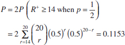
- Conclusions: Because p = 0.1153 is not less than α = 0.05, we cannot reject the null hypothesis that the median shear strength is 2000 psi. Another way to say this is that the observed number of plus signs r+ = 14 was not large or small enough to indicate that median shear strength is different from 2000 psi at the α = 0.05 level of significance.
![]() TABLE • 9-5 Propellant Shear Strength Data
TABLE • 9-5 Propellant Shear Strength Data

It is also possible to construct a table of critical values for the sign test. This table is shown as Appendix Table VIII. Its use for the two-sided alternative hypothesis in Equation 9-54 is simple. As before, let R+ denote the number of the differences (Xi − ![]() 0) that are positive and let R− denote the number of these differences that are negative. Let R = min(R+, R−). Appendix Table VIII presents critical values
0) that are positive and let R− denote the number of these differences that are negative. Let R = min(R+, R−). Appendix Table VIII presents critical values ![]() for the sign test that ensure that P(type I error) = P(reject H0 when H0 is true) = α for α = 0.01, α = 0.05 and α = 0.10. If the observed value of the test statistic r ≤
for the sign test that ensure that P(type I error) = P(reject H0 when H0 is true) = α for α = 0.01, α = 0.05 and α = 0.10. If the observed value of the test statistic r ≤ ![]() the null hypothesis H0:
the null hypothesis H0: ![]() =
= ![]() 0 should be rejected.
0 should be rejected.
To illustrate how this table is used, refer to the data in Table 9-5 that were used in Example 9-15. Now r+ = 14 and r− = 6; therefore, r = min (14, 6) = 6. From Appendix Table VIII with n = 20 and α = 0.05, we find that ![]() = 5. Because r = 6 is not less than or equal to the critical value
= 5. Because r = 6 is not less than or equal to the critical value ![]() = 5, we cannot reject the null hypothesis that the median shear strength is 2000 psi.
= 5, we cannot reject the null hypothesis that the median shear strength is 2000 psi.
We can also use Appendix Table VIII for the sign test when a one-sided alternative hypothesis is appropriate. If the alternative is H1: ![]() >
> ![]() 0 reject H0:
0 reject H0: ![]() =
= ![]() 0 if r− ≤
0 if r− ≤ ![]() ; if the alternative is H1:
; if the alternative is H1: ![]() >
> ![]() 0 reject H0:
0 reject H0: ![]() =
= ![]() 0 if r+ ≤
0 if r+ ≤ ![]() . The level of significance of a one-sided test is one-half the value for a two-sided test. Appendix Table VIII shows the one-sided significance levels in the column headings immediately following the two-sided levels.
. The level of significance of a one-sided test is one-half the value for a two-sided test. Appendix Table VIII shows the one-sided significance levels in the column headings immediately following the two-sided levels.
Finally, note that when a test statistic has a discrete distribution such as R does in the sign test, it may be impossible to choose a critical value ![]() that has a level of significance exactly equal to α. The approach used in Appendix Table VIII is to choose
that has a level of significance exactly equal to α. The approach used in Appendix Table VIII is to choose ![]() to yield an α that is as close to the advertised significance level α as possible.
to yield an α that is as close to the advertised significance level α as possible.
Ties in the Sign Test
Because the underlying population is assumed to be continuous, there is a zero probability that we will find a “tie”—that is, a value of Xi exactly equal to ![]() 0. However, this may sometimes happen in practice because of the way the data are collected. When ties occur, they should be set aside and the sign test applied to the remaining data.
0. However, this may sometimes happen in practice because of the way the data are collected. When ties occur, they should be set aside and the sign test applied to the remaining data.
The Normal Approximation
When p = 0.5, the binomial distribution is well approximated by a normal distribution when n is at least 10. Thus, because the mean of the binomial is np and the variance is np(1 − p), the distribution of R+ is approximately normal with mean 0.5n and variance 0.25n whenever n is moderately large. Therefore, in these cases, the null hypothesis H0: ![]() =
= ![]() 0 can be tested using the statistic
0 can be tested using the statistic
Normal Approximation for Sign Test Statistic

A P-value approach could be used for decision making. The fixed significance level approach could also be used.
The two-sided alternative would be rejected if the observed value of the test statistic |z0| > zα/2, and the critical regions of the one-sided alternative would be chosen to reflect the sense of the alternative. (If the alternative is H1: ![]() >
> ![]() 0, reject H0 if z0 > zα, for example.)
0, reject H0 if z0 > zα, for example.)
Type II Error for the Sign Test
The sign test will control the probability of a type I error at an advertised level α for testing the null hypothesis H0: ![]() =
= ![]() 0 for any continuous distribution. As with any hypothesis-testing procedure, it is important to investigate the probability of a type II error, β. The test should be able to effectively detect departures from the null hypothesis, and a good measure of this effectiveness is the value of β for departures that are important. A small value of β implies an effective test procedure.
0 for any continuous distribution. As with any hypothesis-testing procedure, it is important to investigate the probability of a type II error, β. The test should be able to effectively detect departures from the null hypothesis, and a good measure of this effectiveness is the value of β for departures that are important. A small value of β implies an effective test procedure.
In determining β, it is important to realize not only that a particular value of ![]() , say,
, say, ![]() 0 + Δ, must be used but also that the form of the underlying distribution will affect the calculations. To illustrate, suppose that the underlying distribution is normal with σ = 1 and we are testing the hypothesis H0:
0 + Δ, must be used but also that the form of the underlying distribution will affect the calculations. To illustrate, suppose that the underlying distribution is normal with σ = 1 and we are testing the hypothesis H0: ![]() = 2 versus H1:
= 2 versus H1: ![]() > 2. (Because
> 2. (Because ![]() = μ in the normal distribution, this is equivalent to testing that the mean equals 2.) Suppose that it is important to detect a departure from
= μ in the normal distribution, this is equivalent to testing that the mean equals 2.) Suppose that it is important to detect a departure from ![]() = 2 to
= 2 to ![]() = 3. The situation is illustrated graphically in Fig. 9-18(a). When the alternative hypothesis is true (H1:
= 3. The situation is illustrated graphically in Fig. 9-18(a). When the alternative hypothesis is true (H1: ![]() = 3), the probability that the random variable X is less than or equal to the value 2 is
= 3), the probability that the random variable X is less than or equal to the value 2 is
![]()
Suppose that we have taken a random sample of size 12. At the α = 0.05 level, Appendix Table VIII indicates that we would reject H0: ![]() = 2 if r− ≤
= 2 if r− ≤ ![]() = 2. Therefore, β is the probability that we do not reject H0:μ when in fact
= 2. Therefore, β is the probability that we do not reject H0:μ when in fact ![]() = 3, or
= 3, or
![]()
If the distribution of X had been exponential rather than normal, the situation would be as shown in Fig. 9-18(b), and the probability that the random variable X is less than or equal to the value x = 2 when ![]() = 3 (note that when the median of an exponential distribution is 3, the mean is 4.33) is
= 3 (note that when the median of an exponential distribution is 3, the mean is 4.33) is
![]()
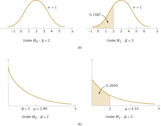
FIGURE 9-18 Calculation of β for the sign test. (a) Normal distributions. (b) Exponential distributions.
In this case,
![]()
Thus, β for the sign test depends not only on the alternative value of ![]() but also on the area to the right of the value specified in the null hypothesis under the population probability distribution. This area depends highly on the shape of that particular probability distribution. In this example, β is large, so the ability of the test to detect this departure from the null hypothesis with the current sample size is poor.
but also on the area to the right of the value specified in the null hypothesis under the population probability distribution. This area depends highly on the shape of that particular probability distribution. In this example, β is large, so the ability of the test to detect this departure from the null hypothesis with the current sample size is poor.
9-9.2 THE WILCOXON SIGNED-RANK TEST
The sign test uses only the plus and minus signs of the differences between the observations and the median ![]() 0 (or the plus and minus signs of the differences between the observations in the paired case). It does not take into account the size or magnitude of these differences. Frank Wilcoxon devised a test procedure that uses both direction (sign) and magnitude. This procedure, now called the Wilcoxon signed-rank test, is discussed and illustrated in this section.
0 (or the plus and minus signs of the differences between the observations in the paired case). It does not take into account the size or magnitude of these differences. Frank Wilcoxon devised a test procedure that uses both direction (sign) and magnitude. This procedure, now called the Wilcoxon signed-rank test, is discussed and illustrated in this section.
The Wilcoxon signed-rank test applies to the case of symmetric continuous distributions. Under these assumptions, the mean equals the median, and we can use this procedure to test the null hypothesis μ = μ0.
The Test Procedure
We are interested in testing H0: μ = μ0 against the usual alternatives. Assume that X1, X2,..., Xn is a random sample from a continuous and symmetric distribution with mean (and median) μ. Compute the differences Xi − μ0, i = 1, 2,..., n. Rank the absolute differences |Xi − μ0|, i = 1,2,..., n in ascending order, and then give the ranks the signs of their corresponding differences. Let W+ be the sum of the positive ranks and W− be the absolute value of the sum of the negative ranks, and let W = min(W+, W−). Appendix Table IX contains critical values of W, say, ![]() . If the alternative hypothesis is H1: μ ≠ μ0, then if the observed value of the statistic w ≤
. If the alternative hypothesis is H1: μ ≠ μ0, then if the observed value of the statistic w ≤ ![]() , the null hypothesis H0: μ = μ0 is rejected. Appendix Table IX provides significance levels of α = 0.10, α = 0.05, α = 0.02 and α = 0.01 for the two-sided test.
, the null hypothesis H0: μ = μ0 is rejected. Appendix Table IX provides significance levels of α = 0.10, α = 0.05, α = 0.02 and α = 0.01 for the two-sided test.
For one-sided tests, if the alternative is H1: μ > μ0, reject H0: μ = μ0 if w− ≤ ![]() ; and if the alternative is H1: μ < μ0, reject H0: μ = μ if w+ ≤
; and if the alternative is H1: μ < μ0, reject H0: μ = μ if w+ ≤ ![]() . The significance levels for one-sided tests provided in Appendix Table IX are α = 0.05, 0.025, 0.01, and 0.005.
. The significance levels for one-sided tests provided in Appendix Table IX are α = 0.05, 0.025, 0.01, and 0.005.
Example 9-16 Propellant Shear Strength-Wilcoxon Signed-Rank Test We will illustrate the Wilcoxon signed-rank test by applying it to the propellant shear strength data from Table 9-5. Assume that the underlying distribution is a continuous symmetric distribution. The seven-step procedure is applied as follows:
- Parameter of interest: The parameter of interest is the mean (or median) of the distribution of propellant shear strength.
- Null hypothesis: H0: μ = 2000 psi
- Alternative hypothesis: H0: μ ≠ 2000 psi
- Test statistic: The test statistic is w = min(w+, w−)
- Reject H0 if: We will reject H0 if w ≤
 = 52 from Appendix Table IX.
 - Computations: The signed ranks from Table 9-5 are shown in the following display:
The sum of the positive ranks is w+ = (1 + 2 + 3 + 4 + 5 + 6 + 11 + 13 + 15 + 16 + 17 + 18 + 19 + 20) = 150, and the sum of the absolute values of the negative ranks is w- = (7 + 8 + 9 + 10 + 12 + 14) = 60. Therefore,
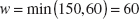

- Conclusions: Because w = 60 is not less than or equal to the critical value w0.05 = 52, we cannot reject the null hypothesis that the mean (or median, because the population is assumed to be symmetric) shear strength is 2000 psi.
Ties in the Wilcoxon Signed-Rank Test
Because the underlying population is continuous, ties are theoretically impossible, although they will sometimes occur in practice. If several observations have the same absolute magnitude, they are assigned the average of the ranks that they would receive if they differed slightly from one another.
Large Sample Approximation
If the sample size is moderately large, say, n > 20, it can be shown that W+ (or W−) has approximately a normal distribution with mean
![]()
and variance
![]()
Therefore, a test of H0: μ = μ0 can be based on the statistic:
Normal Approximation for Wilcoxon Signed-Rank Statistic
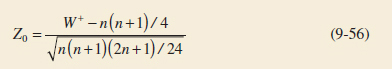
An appropriate critical region for either the two-sided or one-sided alternative hypotheses can be chosen from a table of the standard normal distribution.
9-9.3 COMPARISON TO THE T-TEST
If the underlying population is normal, either the sign test or the t-test could be used to test a hypothesis about the population median. The t-test is known to have the smallest value of β possible among all tests that have significance level α for the one-sided alternative and for tests with symmetric critical regions for the two-sided alternative, so it is superior to the sign test in the normal distribution case. When the population distribution is symmetric and non-normal (but with finite mean), the t-test will have a smaller β (or a higher power) than the sign test unless the distribution has very heavy tails compared with the normal. Thus, the sign test is usually considered a test procedure for the median rather than as a serious competitor for the t-test. The Wilcoxon signed-rank test is preferable to the sign test and compares well with the t-test for symmetric distributions. It can be useful for situations in which a transformation on the observations does not produce a distribution that is reasonably close to the normal.
EXERCISES FOR SECTION 9-9
![]() Problem available in WileyPLUS at instructor's discretion.
Problem available in WileyPLUS at instructor's discretion.
![]() Go Tutorial Tutoring problem available in WileyPLUS at instructor's discretion.
Go Tutorial Tutoring problem available in WileyPLUS at instructor's discretion.
9-122. ![]() Ten samples were taken from a plating bath used in an electronics manufacturing process, and the bath pH of the bath was determined. The sample pH values are 7.91, 7.85, 6.82, 8.01, 7.46, 6.95, 7.05, 7.35, 7.25, and 7.42. Manufacturing engineering believes that pH has a median value of 7.0.
Ten samples were taken from a plating bath used in an electronics manufacturing process, and the bath pH of the bath was determined. The sample pH values are 7.91, 7.85, 6.82, 8.01, 7.46, 6.95, 7.05, 7.35, 7.25, and 7.42. Manufacturing engineering believes that pH has a median value of 7.0.
(a) Do the sample data indicate that this statement is correct? Use the sign test with α = 0.05 to investigate this hypothesis. Find the P-value for this test.
(b) Use the normal approximation for the sign test to test H0: ![]() = 7.0 versus H0:
= 7.0 versus H0: ![]() ≠ 7.0. What is the P-value for this test?
≠ 7.0. What is the P-value for this test?
9-123. ![]() The titanium content in an aircraft-grade alloy is an important determinant of strength. A sample of 20 test coupons reveals the following titanium content (in percent):
The titanium content in an aircraft-grade alloy is an important determinant of strength. A sample of 20 test coupons reveals the following titanium content (in percent):
8.32, 8.05, 8.93, 8.65, 8.25, 8.46, 8.52, 8.35, 8.36, 8.41, 8.42, 8.30, 8.71, 8.75, 8.60, 8.83, 8.50, 8.38, 8.29, 8.46
The median titanium content should be 8.5%.
(a) Use the sign test with α = 0.05 to investigate this hypothesis. Find the P-value for this test.
(b) Use the normal approximation for the sign test to test H0: ![]() = 8.5 versus H1:
= 8.5 versus H1: ![]() ≠ 8.5 with α = 0.05. What is the P-value for this test?
≠ 8.5 with α = 0.05. What is the P-value for this test?
9-124. ![]() The impurity level (in ppm) is routinely measured in an intermediate chemical product. The following data were observed in a recent test:
The impurity level (in ppm) is routinely measured in an intermediate chemical product. The following data were observed in a recent test:
2.4, 2.5, 1.7, 1.6, 1.9, 2.6, 1.3, 1.9, 2.0, 2.5, 2.6, 2.3, 2.0, 1.8, 1.3, 1.7, 2.0, 1.9, 2.3, 1.9, 2.4, 1.6
Can you claim that the median impurity level is less than 2.5 ppm?
(a) State and test the appropriate hypothesis using the sign test with α = 0.05. What is the P-value for this test?
(b) Use the normal approximation for the sign test to test H0: ![]() = 2.5 versus H1:
= 2.5 versus H1: ![]() < 2.5. What is the P-value for this test?
< 2.5. What is the P-value for this test?
9-125. ![]() Consider the margarine fat content data in Exercise 8-36. Use the sign test to test H0:
Consider the margarine fat content data in Exercise 8-36. Use the sign test to test H0: ![]() = 17.0 versus H1:
= 17.0 versus H1: ![]() ≠ 17.0 with α = 0.05.
≠ 17.0 with α = 0.05.
(a) Find the P-value for the test statistic and use this quantity to make your decision.
(b) Use the normal approximation to test the same hypothesis that you formulated in part (a). What is the P-value for this test?
9-126. ![]() Consider the compressive strength data in Exercise 8-62.
Consider the compressive strength data in Exercise 8-62.
(a) Use the sign test to investigate the claim that the median strength is at least 2250 psi. Use α = 0.05.
(b) Use the normal approximation to test the same hypothesis that you formulated in part (a). What is the P-value for this test?
9-127. ![]() An inspector are measured the diameter of a ball bearing using a new type of caliper. The results were as follows (in mm): 0.265, 0.263, 0.266, 0.267, 0.267, 0.265, 0.267, 0.267, 0.265, 0.268, 0.268, and 0.263.
An inspector are measured the diameter of a ball bearing using a new type of caliper. The results were as follows (in mm): 0.265, 0.263, 0.266, 0.267, 0.267, 0.265, 0.267, 0.267, 0.265, 0.268, 0.268, and 0.263.
(a) Use the Wilcoxon signed-rank test to evaluate the claim that the mean ball diameter is 0.265 mm. Use α = 0.05.
(b) Use the normal approximation for the test. With α = 0.05, what conclusions can you draw?
9-128. ![]() A new type of tip can be used in a Rockwell hardness tester. Eight coupons from test ingots of a nickel-based alloy are selected, and each coupon is tested using the new tip. The Rockwell C-scale hardness readings are 63, 65, 58, 60, 55, 57, 53, and 59. Do the results support the claim that the mean hardness exceeds 60 at a 0.05 level?
A new type of tip can be used in a Rockwell hardness tester. Eight coupons from test ingots of a nickel-based alloy are selected, and each coupon is tested using the new tip. The Rockwell C-scale hardness readings are 63, 65, 58, 60, 55, 57, 53, and 59. Do the results support the claim that the mean hardness exceeds 60 at a 0.05 level?
9-129. ![]() A primer paint can be used on aluminum panels. The primer's drying time is an important consideration in the manufacturing process. Twenty panels are selected, and the drying times are as follows: 1.6, 1.3, 1.5, 1.6, 1.7, 1.9, 1.8, 1.6, 1.4, 1.8, 1.9, 1.8, 1.7, 1.5, 1.6, 1.4, 1.3, 1.6, 1.5, and 1.8. Is there evidence that the mean drying time of the primer exceeds 1.5 hr?
A primer paint can be used on aluminum panels. The primer's drying time is an important consideration in the manufacturing process. Twenty panels are selected, and the drying times are as follows: 1.6, 1.3, 1.5, 1.6, 1.7, 1.9, 1.8, 1.6, 1.4, 1.8, 1.9, 1.8, 1.7, 1.5, 1.6, 1.4, 1.3, 1.6, 1.5, and 1.8. Is there evidence that the mean drying time of the primer exceeds 1.5 hr?
9-10 Equivalence Testing
Statistical hypothesis testing is one of the most useful techniques of statistical inference. However, it works in only one direction; that is, it starts with a statement that is assumed to be true (the null hypothesis H0) and attempts to disprove this claim in favor of the alternative hypothesis H1. The strong statement about the alternative hypothesis is made when the null hypothesis is rejected. This procedure works well in many but not all situations.
To illustrate, consider a situation in which we are trying to qualify a new supplier of a component that we use in manufacturing our product. The current supplier produces these components with a standard mean resistance of 80 ohms. If the new supplier can provide components with the same mean resistance, we will qualify them. Having a second source for this component is considered to be important because demand for our product is expected to grow rapidly in the near future, and the second supplier will be necessary to meet the anticipated increase in demand. The traditional formulation of the hypothesis test
![]()
really is not satisfactory. Only if we reject the null hypothesis do we have a strong conclusion. We actually want to state the hypotheses as follows:
![]()
This type of hypothesis statement is called an equivalence test. We assume that the new supplier is different from the standard unless we have strong evidence to reject that claim. The way that this equivalence test is carried out is to test the following two sets of one-sided alternative hypotheses:
![]()
and
![]()
where δ is called the equivalence band, which is a practical threshold or limit within which the mean performance (here the resistance) is considered to be the same as the standard. The interval 80±δ is called an equivalence interval. The first set of hypotheses is a test of the mean that shows that the difference between the mean and the standard is significantly less than the upper equivalence limit of the interval, and the second set of hypotheses is a test of the mean that shows that the difference between the mean and the standard is significantly greater than the lower equivalence limit. We are going to apply both tests to the same sample of data, leading to a test of equivalence that is sometimes called two one-sided tests (TOST).
Example 9-17 Suppose that we have a random sample of n = 50 components from the new supplier. Resistance is approximately normally distributed, and the sample mean and standard deviation (in ohms) are ![]() = 79.98 and s = 0.10. The sample mean is close to the standard of 80 ohms. Suppose that our error of measurement is approximately 0.01 ohm. We will decide that if the new supplier has a mean resistance that is within 0.05 of the standard of 80, there is no practical difference in performance. Therefore, δ = 0.05. Notice that we have chosen the equivalence band to be greater than the usual or expected measurement error for the resistance. We now want to test the hypotheses
= 79.98 and s = 0.10. The sample mean is close to the standard of 80 ohms. Suppose that our error of measurement is approximately 0.01 ohm. We will decide that if the new supplier has a mean resistance that is within 0.05 of the standard of 80, there is no practical difference in performance. Therefore, δ = 0.05. Notice that we have chosen the equivalence band to be greater than the usual or expected measurement error for the resistance. We now want to test the hypotheses
![]()
and
![]()
Consider testing the first set of hypotheses. It is straightforward to show that the value of the test statistic is t0 = −4.95, and the P-value is less than 0.01. Therefore, we conclude that the mean resistance is less than 80.05. For the second set of hypotheses, the test statistic is t0 = 2.12, and the P-value is less than 0.025, so the mean resistance is significantly greater than 79.95 and significantly less than 80.05. Thus, we have enough evidence to conclude that the new supplier produces components that are equivalent to those produced by the current supplier because the mean is within the ±0.05 ohm interval.
Equivalence testing has many applications, including the supplier qualification problem illustrated here, generic drug manufacturing, and new equipment qualification. The experimenter must decide what defines equivalence. Issues that should be considered include these:
- Specifying the equivalence band. The parameter δ should be larger than the typical measurement error. A good rule of thumb is that δ should be at least three times the typical measurement error.
- The equivalence band should be much smaller than the usual process variation.
- The equivalence band should be much smaller than the product or process specifications. Specifications typically define fitness for use.
- The equivalence band should be related to actual functional performance; that is, how much of a difference can be tolerated before performance is degraded?
Exercises FOR SECTION 9-10
![]() Problem available in WileyPLUS at instructor's discretion.
Problem available in WileyPLUS at instructor's discretion.
![]() Go Tutorial Tutoring problem available in WileyPLUS at instructor's discretion.
Go Tutorial Tutoring problem available in WileyPLUS at instructor's discretion.
9-130. In developing a generic drug, it is necessary for a manufacturer of biopharmaceutical products to show equivalence to the current product. The variable of interest is the absorption rate of the product. The current product has an absorption rate of 18 mg/hr. If the new generic product has an absorption rate that is within 0.50 mg/hr of this value, it will be considered equivalent. A random sample of 20 units of product is available, and the sample mean and standard deviation of absorption rate are 18.22 mg/hr and 0.92 mg/hr, respectively.
(a) State the appropriate hypotheses that must be tested to demonstrate equivalence.
(b) What are your conclusions using α = 0.05?
9-131. A chemical products manufacturer must identify a new supplier for a raw material that is an essential component of a particular product. The previous supplier was able to deliver material with a mean molecular weight of 3500. The new supplier must show equivalence to this value of molecular weight. If the new supplier can deliver material that has a molecular weigh that is within 50 units of this value, it will be considered equivalent. A random sample of 10 lots of product is available, and the sample mean and standard deviation of molecular weight are 3550 and 25, respectively.
(a) State the appropriate hypotheses that must be tested to demonstrate equivalence.
(b) What are your conclusions using α = 0.05?
9-132. The mean breaking strength of a ceramic insulator must be at least 10 psi. The process by which this insulator is manufactured must show equivalence to this standard. If the process can manufacture insulators with a mean breaking strength of at least 9.5 psi, it will be considered equivalent to the standard. A random sample of 50 insulators is available, and the sample mean and standard deviation of breaking strength are 9.31 psi and 0.22 psi, respectively.
(a) State the appropriate hypotheses that must be tested to demonstrate equivalence.
(b) What are your conclusions using α = 0.05?
9-133. The mean bond strength of a cement product must be at least 1000 psi. The process by which this material is manufactured must show equivalence to this standard. If the process can manufacture cement for which the mean bond strength is at least 9750 psi, it will be considered equivalent to the standard. A random sample of six observations is available, and the sample mean and standard deviation of bond strength are 9360 psi and 42.6 psi, respectively.
(a) State the appropriate hypotheses that must be tested to demonstrate equivalence.
(b) What are your conclusions using α = 0.05?
9-11 Combining P-Values
Testing several sets of hypotheses that relate to a problem of interest occurs fairly often in engineering and many scientific disciplines. For example, suppose that we are developing a new synthetic fiber to be used in manufacturing body armor for the military and law enforcement agencies. This fiber needs to exhibit a high breaking strength (at least 100 lb/in2) for the new product to work properly. The engineering development lab produced several batches or lots of this fiber, a random sample of three fiber specimens from each lot has been taken, and the sample specimens tested. For each lot, the hypotheses of interest are
![]()
The development lots are small, and the testing is destructive, so the sample sizes are also small. After six lots have been produced, the P-values from these six independent tests of hypotheses are 0.105, 0.080, 0.250, 0.026, 0.650, and 0.045. Given the size of these P-values, we suspect that the new material is going to be satisfactory, but the sample sizes are small, and it would be helpful if we could combine the results from all six tests to determine whether the new material will be acceptable. Combining results from several studies or experiments is sometimes called meta-analysis, a technique that has been used in many fields including public health monitoring, clinical trials of new medical devices or treatments, ecology, and genetics. One method that can be used to combine these results is to combine all of the individual P-values into a single statistic for which one P-value can be computed. This procedure was developed by R. A. Fisher.
Let Pi be the P-value for the ith set of hypotheses, i = 1, 2,..., m. The test statistic is
![]()
The test statistic ![]() follows a chi-square distribution with 2m degrees of freedom. A P-value can be computed for the observed value of this statistic. A small P-value would lead to rejection of the shared null hypotheses and a conclusion that the combined data support the alternative.
follows a chi-square distribution with 2m degrees of freedom. A P-value can be computed for the observed value of this statistic. A small P-value would lead to rejection of the shared null hypotheses and a conclusion that the combined data support the alternative.
As an example, the test statistic ![]() for the six tests described is
for the six tests described is
![]()
with 2m = 2(6) = 12 degrees of freedom. The P-value for this statistic is 0.005 < P < 0.01, a very small value, which leads to rejection of the null hypothesis. In other words, the combined information from all six tests provides evidence that the mean fiber strength exceeds 100 lb/in2.
Fisher's method does not require all the null hypotheses be the same. Some applications involve many sets of hypotheses that do not have the same null. In these situations, the alternative hypothesis is taken to be that at least one of the null hypotheses is false. Fisher's method was developed in the 1920s. Since then, a number of other techniques has been proposed. For a good discussion of these alternative methods along with comments on their appropriateness and power, see the article by Piegorsch and Bailer [“Combining Information,” Wiley Interdiscip Rev Comput Stat, 2009, Vol. 1(3), pp. 354–360].
Exercises FOR SECTION 9-10
![]() Problem available in WileyPLUS at instructor's discretion.
Problem available in WileyPLUS at instructor's discretion.
![]() Go Tutorial Tutoring problem available in WileyPLUS at instructor's discretion.
Go Tutorial Tutoring problem available in WileyPLUS at instructor's discretion.
9-134. Suppose that 10 sets of hypotheses of the form
![]()
have been tested and that the P-values for these tests are 0.12, 0.08. 0.93, 0.02, 0.01, 0.05, 0.88, 0.15, 0.13, and 0.06. Use Fisher's procedure to combine all of these P-values. What conclusions can you draw about these hypotheses?
9-135. Suppose that eight sets of hypotheses about a population proportion of the form
![]()
have been tested and that the P-values for these tests are 0.15, 0.83, 0.103, 0.024, 0.03, 0.07, 0.09, and 0.13. Use Fisher's procedure to combine all of these P-values. Is there sufficient evidence to conclude that the population proportion exceeds 0.30?
9-136. The standard deviation of fill volume of a container of a pharmaceutical product must be less than 0.2 oz to ensure that the container is accurately filled. Six independent samples were selected, and the statistical hypotheses about the standard deviation were tested. The P-values that resulted were 0.15, 0.091, 0.075, 0.02, 0.04, and 0.06. Is there sufficient evidence to conclude that the standard deviation of fill volume is less than 0.2 oz?
9-137. The mean weight of a package of frozen fish must equal 22 oz. Five independent samples were selected, and the statistical hypotheses about the mean weight were tested. The P-values that resulted from these tests were 0.065, 0.0924, 0.073, 0.025, and 0.021. Is there sufficient evidence to conclude that the mean package weight is not equal to 22 oz?
Supplemental Exercises
![]() Problem available in WileyPLUS at instructor's discretion.
Problem available in WileyPLUS at instructor's discretion.
![]() Go Tutorial Tutoring problem available in WileyPLUS at instructor's discretion.
Go Tutorial Tutoring problem available in WileyPLUS at instructor's discretion.
9-138. Consider the following computer output.
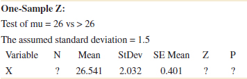
(a) Fill in the missing information.
(b) Is this a one-sided or a two-sided test?
(c) What are your conclusions if α = 0.05?
(d) Find a 95% two-sided CI on the mean.
9-139. ![]() Consider the following computer output.
Consider the following computer output.
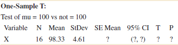
(a) How many degrees of freedom are there on the t-statistic?
(b) Fill in the missing information. You may use bounds on the P-value.
(c) What are your conclusions if α = 0.05?
(d) What are your conclusions if the hypothesis is H0: μ = 100 versus H0: μ > 100?
9-140. Consider the following computer output.

(a) How many degrees of freedom are there on the t-statistic?
(b) Fill in the missing information. You may use bounds on the P-value.
(c) What are your conclusions if α = 0.05?
(d) Find a 95% upper-confidence bound on the mean.
(e) What are your conclusions if the hypothesis is H0: μ = 100 versus H0: μ > 100?
9-141. An article in Transfusion Science [“Early Total White Blood Cell Recovery Is a Predictor of Low Number of Apheresis and Good CD34+ Cell Yield” (2000, Vol. 23, pp. 91–100)] studied the white blood cell recovery of patients with haematological malignancies after a new chemotherapy treatment. Data (in days) on white blood cell recovery (WBC) for 19 patients consistent with summary data reported in the paper follow: 18, 16, 13, 16, 15, 12, 9, 14, 12, 8, 16, 12, 10, 8, 14, 9, 5, 18, and 12.
(a) Is there sufficient evidence to support a claim that the mean WBC recovery exceeds 12 days?
(b) Find a 95% two-sided CI on the mean WBC recovery.
9-142. An article in Fire Technology [“An Experimental Examination of Dead Air Space for Smoke Alarms” (2009, Vol. 45, pp. 97–115)] studied the performance of smoke detectors installed not less than 100 mm from any adjoining wall if mounted on a flat ceiling, and not closer than 100 mm and not farther than 300 mm from the adjoining ceiling surface if mounted on walls. The purpose of this rule is to avoid installation of smoke alarms in the “dead air space,” where it is assumed to be difficult for smoke to reach. The paper described a number of interesting experiments. Results on the time to signal (in seconds) for one such experiment with pine stick fuel in an open bedroom using photoelectric smoke alarms are as follows: 220, 225, 297, 315, 282, and 313.
(a) Is there sufficient evidence to support a claim that the mean time to signal is less than 300 seconds?
(b) Is there practical concern about the assumption of a normal distribution as a model for the time-to-signal data?
(c) Find a 95% two-sided CI on the mean time to signal.
9-143. Suppose that we wish to test the hypothesis H0: μ = 85 versus the alternative H1: μ > 85 where σ = 16. Suppose that the true mean is μ = 86 and that in the practical context of the problem, this is not a departure from μ0 = 85 that has practical significance.
(a) For a test with α = 0.01, compute β for the sample sizes n = 25, 100, 400, and 2500 assuming that μ = 86.
(b) Suppose that the sample average is ![]() = 86. Find the P-value for the test statistic for the different sample sizes specified in part (a). Would the data be statistically significant at α = 0.01?
= 86. Find the P-value for the test statistic for the different sample sizes specified in part (a). Would the data be statistically significant at α = 0.01?
(c) Comment on the use of a large sample size in this problem.
9-144. A manufacturer of semiconductor devices takes a random sample of size n of chips and tests them, classifying each chip as defective or nondefective. Let Xi = 0 if the chip is nondefective and Xi = 1 if the chip is defective. The sample fraction defective is
![]()
What are the sampling distribution, the sample mean, and sample variance estimates of ![]() when
when
(a) The sample size is n = 50?
(b) The sample size is n = 80?
(c) The sample size is n = 100?
(d) Compare your answers to parts (a)–(c) and comment on the effect of sample size on the variance of the sampling distribution.
9-145. Consider the situation of Exercise 9-144. After collecting a sample, we are interested in testing H0: p = 0.10 versus H1: p ≠ 0.10 with α = 0.05. For each of the following situations, compute the p-value for this test:
(a) n = 50, ![]() = 0.095
= 0.095
(b) n = 100, ![]() = 0.095
= 0.095
(c) n = 500, ![]() = 0.095
= 0.095
(d) n = 1000, ![]() = 0.095
= 0.095
(e) Comment on the effect of sample size on the observed P-value of the test.
9-146. An inspector of flow metering devices used to administer fluid intravenously will perform a hypothesis test to determine whether the mean flow rate is different from the flow rate setting of 200 milliliters per hour. Based on prior information, the standard deviation of the flow rate is assumed to be known and equal to 12 milliliters per hour. For each of the following sample sizes, and a fixed α = 0.05, find the probability of a type II error if the true mean is 205 milliliters per hour.
(a) n = 20
(b) n = 50
(c) n = 100
(d) Does the probability of a type II error increase or decrease as the sample size increases? Explain your answer.
9-147. Suppose that in Exercise 9-146, the experimenter had believed that σ = 14. For each of the following sample sizes, and a fixed α = 0.05, find the probability of a type II error if the true mean is 205 milliliters per hour.
(a) n = 20
(b) n = 50
(c) n = 100
(d) Comparing your answers to those in Exercise 9-46, does the probability of a type II error increase or decrease with the increase in standard deviation? Explain your answer.
9-148. The marketers of shampoo products know that customers like their product to have a lot of foam. A manufacturer of shampoo claims that the foam height of its product exceeds 200 millimeters. It is known from prior experience that the standard deviation of foam height is 8 millimeters. For each of the following sample sizes and with a fixed α = 0.05, find the power of the test if the true mean is 204 millimeters.
(a) n = 20
(b) n = 50
(c) n = 100
(d) Does the power of the test increase or decrease as the sample size increases? Explain your answer.
9-149. Suppose that you are testing H0: p = 0.5 versus H0: p ≠ 0.5. Suppose that p is the true value of the population proportion.
(a) Using α = 0.05, find the power of the test for n = 100, 150, and 300 assuming that p = 0.6. Comment on the effect of sample size on the power of the test.
(b) Using α = 0.01, find the power of the test for n = 100, 150, and 300 assuming that p = 0.6. Compare your answers to those from part (a) and comment on the effect of α on the power of the test for different sample sizes.
(c) Using α = 0.05, find the power of the test for n = 100, assuming p = 0.08. Compare your answer to part (a) and comment on the effect of the true value of p on the power of the test for the same sample size and α level.
(d) Using α = 0.01, what sample size is required if p = 0.6 and we want β = 0.05? What sample is required if p = 0.8 and we want β = 0.05? Compare the two sample sizes and comment on the effect of the true value of p on a sample size required when β is held approximately constant.
9-150. The cooling system in a nuclear submarine consists of an assembly of welded pipes through which a coolant is circulated. Specifications require that weld strength must meet or exceed 150 psi.
(a) Suppose that the design engineers decide to test the hypothesis H0: μ = 150 versus H1: μ > 150. Explain why this choice of alternative hypothesis is better than H1: μ < 150.
(b) A random sample of 20 welds results in ![]() = 153.7 psi and s = 11.3 psi. What conclusions can you draw about the hypothesis in part (a)? State any necessary assumptions about the underlying distribution of the data.
= 153.7 psi and s = 11.3 psi. What conclusions can you draw about the hypothesis in part (a)? State any necessary assumptions about the underlying distribution of the data.
9-151. The mean pull-off force of an adhesive used in manufacturing a connector for an automotive engine application should be at least 75 pounds. This adhesive will be used unless there is strong evidence that the pull-off force does not meet this requirement. A test of an appropriate hypothesis is to be conducted with sample size n = 10 and α = 0.05. Assume that the pull-off force is normally distributed, and σ is not known.
(a) If the true standard deviation is σ = 1, what is the risk that the adhesive will be judged acceptable when the true mean pull-off force is only 73 pounds? Only 72 pounds?
(b) What sample size is required to give a 90% chance of detecting that the true mean is only 72 pounds when σ = 1?
(c) Rework parts (a) and (b) assuming that σ = 2. How much impact does increasing the value of σ have on the answers you obtain?
9-152. A manufacturer of precision measuring instruments claims that the standard deviation in the use of the instruments is at most 0.00002 millimeter. An analyst who is unaware of the claim uses the instrument eight times and obtains a sample standard deviation of 0.00001 millimeter.
(a) Confirm using a test procedure and an α level of 0.01 that there is insufficient evidence to support the claim that the standard deviation of the instruments is at most 0.00002. State any necessary assumptions about the underlying distribution of the data.
(b) Explain why the sample standard deviation, s = 0.00001, is less than 0.00002, yet the statistical test procedure results do not support the claim.
9-153. A biotechnology company produces a therapeutic drug whose concentration has a standard deviation of 4 grams per liter. A new method of producing this drug has been proposed, although some additional cost is involved. Management will authorize a change in production technique only if the standard deviation of the concentration in the new process is less than 4 grams per liter. The researchers chose n = 10 and obtained the following data in grams per liter. Perform the necessary analysis to determine whether a change in production technique should be implemented.
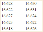
9-154. Consider the 40 observations collected on the number of nonconforming coil springs in production batches of size 50 given in Exercise 6-114.
(a) Based on the description of the random variable and these 40 observations, is a binomial distribution an appropriate model? Perform a goodness-of-fit procedure with α = 0.05.
(b) Calculate the P-value for this test.
9-155. Consider the 20 observations collected on the number of errors in a string of 1000 bits of a communication channel given in Exercise 6-115.
(a) Based on the description of the random variable and these 20 observations, is a binomial distribution an appropriate model? Perform a goodness-of-fit procedure with α = 0.05.
(b) Calculate the P-value for this test.
9-156. Consider the spot weld shear strength data in Exercise 6-39. Does the normal distribution seem to be a reasonable model for these data? Perform an appropriate goodness-of-fit test to answer this question.
9-157. Consider the water quality data in Exercise 9-157.
(a) Do these data support the claim that the mean concentration of suspended solids does not exceed 50 parts per million? Use α = 0.05.
(b) What is the P-value for the test in part (a)?
(c) Does the normal distribution seem to be a reasonable model for these data? Perform an appropriate goodness-of-fit test to answer this question.
9-158. Consider the golf ball overall distance data in Exercise 6-41.
(a) Do these data support the claim that the mean overall distance for this brand of ball does not exceed 270 yards? Use α = 0.05.
(b) What is the P-value for the test in part (a)?
(c) Do these data appear to be well modeled by a normal distribution? Use a formal goodness-of-fit test in answering this question.
9-159. Consider the baseball coefficient of restitution data in Exercise 8-103. If the mean coefficient of restitution exceeds 0.635, the population of balls from which the sample has been taken will be too “lively” and considered unacceptable for play.
(a) Formulate an appropriate hypothesis testing procedure to answer this question.
(b) Test these hypotheses and draw conclusions, using α = 0.01.
(c) Find the P-value for this test.
(d) In Exercise 8-103(b), you found a 99% confidence interval on the mean coefficient of restitution. Does this interval or a one-sided CI provide additional useful information to the decision maker? Explain why or why not.
9-160. Consider the dissolved oxygen data in Exercise 8-105. Water quality engineers are interested in knowing whether these data support a claim that mean dissolved oxygen concentration is 2.5 milligrams per liter.
(a) Formulate an appropriate hypothesis testing procedure to investigate this claim.
(b) Test these hypotheses and draw conclusions, using α = 0.05.
(c) Find the P-value for this test.
(d) In Exercise 8-105(b), you found a 95% CI on the mean dissolved oxygen concentration. Does this interval provide useful additional information beyond that of the hypothesis testing results? Explain your answer.
9-161. An article in Food Testing and Analysis [“Improving Reproducibility of Refractometry Measurements of Fruit Juices” (1999, Vol. 4(4), pp. 13–17)] measured the sugar concentration (Brix) in clear apple juice. All readings were taken at 20°C:
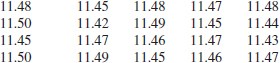
(a) Test the hypothesis H0: μ = 11.5 versus H1: μ ≠ 11.5 using α = 0.05. Find the P-value.
(b) Compute the power of the test if the true mean is 11.4.
(c) What sample size would be required to detect a true mean sugar concentration of 11.45 if we wanted the power of the test to be at least 0.9?
(d) Explain how the question in part (a) could be answered by constructing a two-sided confidence interval on the mean sugar concentration.
(e) Is there evidence to support the assumption that the sugar concentration is normally distributed?
9-162. Consider the computer output below
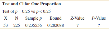
Using the normal approximation:
(a) Fill in the missing information.
(b) What are your conclusions if α = 0.05?
(c) The normal approximation to the binomial was used here. Was that appropriate?
(d) Find a 95% upper-confidence bound on the true proportion.
(e) What are the P-value and your conclusions if the alternative hypothesis is H1: p ≠ 0.25?
9-163. An article in Food Chemistry [“A Study of Factors Affecting Extraction of Peanut (Arachis Hypgaea L.) Solids with Water” (1991, Vol. 42(2), pp. 153–165)] reported that the percent protein extracted from peanut milk as follows:
![]()
(a) Can you support a claim that the mean percent protein extracted exceeds 80 percent? Use α = 0.05.
(b) Is there evidence that the percent protein extracted is normally distributed?
(c) What is the P-value of the test statistic computed in part (a)?
9-164. An article in Biological Trace Element Research [“Interaction of Dietary Calcium, Manganese, and Manganese Source (Mn Oxide or Mn Methionine Complex) or Chick Performance and Manganese Utilization” (1991, Vol. 29(3), pp. 217–228)] showed the following results of tissue assay for liver manganese (ppm) in chicks fed high Ca diets.
![]()
(a) Test the hypothesis H0: σ2 = 0.6 versus H1: σ2 ≠ 0.6 using α = 0.01.
(b) What is the P-value for this test?
(c) Discuss how part (a) could be answered by constructing a 99% two-sided confidence interval for σ.
9-165. An article in Experimental Brain Research [“Synapses in the Granule Cell Layer of the Rat Dentate Gyrus: Serial-Sectionin Study” (1996, Vol. 112(2), pp. 237–243)] showed the ratio between the numbers of symmetrical and total synapses on somata and azon initial segments of reconstructed granule cells in the dentate gyrus of a 12-week-old rat:
(a) Use the data to test H0:σ2 = 0.02 versus H1:σ2 ≠ 0.02 using α = 0.05.
(b) Find the P-value for the test.
9-166. An article in the Journal of Electronic Material [“Progress in CdZnTe Substrate Producibility and Critical Drive of IRFPA Yield Originating with CdZnTe Substrates” (1998, Vol. 27(6), pp. 564–572)] improved the quality of CdZnTe substrates used to produce the HgCdTe infrared focal plane arrays (IRFPAs) also defined as sensor chip assemblies (SCAs). The cut-on wavelength (μm) on 11 wafers was measured and follows:
![]()
(a) Is there evidence that the mean of cut-on wavelength is not 6.50 μm?
(b) What is the P-value for this test?
(c) What sample size would be required to detect a true mean cut-on wavelength of 6.25 μm with probability 95%?
(d) What is the type II error probability if the true mean cut-on wavelength is 6.95 μm?
9-167. Consider the fatty acid measurements for the diet margarine described in Exercise 8-38.
(a) For the sample size n = 6, using a two-sided alternative hypothesis and α = 0.01, test H0: σ2 = 1.0.
(b) Suppose that instead of n = 6, the sample size was n = 51. Repeat the analysis performed in part (a) using n = 51.
(c) Compare your answers and comment on how sample size affects your conclusions drawn in parts (a) and (b).
9-168. Consider the television picture tube brightness experiment described in Exercise 8-37.
(a) For the sample size n = 10, do the data support the claim that the standard deviation of current is less than 20 microamps?
(b) Suppose that instead of n = 10, the sample size was 51. Repeat the analysis performed in part (a) using n = 51.
(c) Compare your answers and comment on how sample size affects your conclusions drawn in parts (a) and (b).
9-169. A manufacturer of a pharmaceutical product is developing a generic drug and must show its the equivalence to the current product. The variable of interest is the activity level of the active ingredient. The current product has an activity level of 100. If the new generic product has an activity level that is within 2 units of this value, it will be considered equivalent. A random sample of 10 units of product is available, and the sample mean and standard deviation of absorption rate are 96 and 1.5, respectively.
(a) State the appropriate hypotheses that must be used to demonstrate equivalence.
(b) What are your conclusions using α = 0.05?
9-170. Suppose that eight sets of hypotheses of the form
![]()
have been tested and that the P-values for these tests are 0.15, 0.06. 0.67, 0.01, 0.04, 0.08, 0.78, and 0.13. Use Fisher's procedure to combine all of the P-values. What conclusions can you draw about these hypotheses?
Mind-Expanding Exercises
9-171. Suppose that we wish to test H0: μ = μ0 versus H1: μ ≠ μ0 where the population is normal with known σ. Let 0 < ![]() < α, and define the critical region so that we will reject H0 if z0 > zε or if z0 < − zα−ε, where z0 is the value of the usual test statistic for these hypotheses.
< α, and define the critical region so that we will reject H0 if z0 > zε or if z0 < − zα−ε, where z0 is the value of the usual test statistic for these hypotheses.
(a) Show that the probability of type I error for this test is α.
(b) Suppose that the true mean is μ1 = μ0 + δ. Derive an expression for β for the above test.
9-172. Derive an expression for β for the test on the variance of a normal distribution. Assume that the two-sided alternative is specified.
9-173. When X1, X2,..., Xn are independent Poisson random variables, each with parameter λ, and n is large, the sample mean ![]() has an approximate normal distribution with mean λ and variance λ/n. Therefore,
has an approximate normal distribution with mean λ and variance λ/n. Therefore,
![]()
has approximately a standard normal distribution. Thus, we can test H0: λ = λ0 by replacing λ in Z by λ0. When Xi are Poisson variables, this test is preferable to the large-sample test of Section 9-2.3, which would use S/![]() in the denominator because it is designed just for the Poisson distribution. Suppose that the number of open circuits on a semiconductor wafer has a Poisson distribution. Test data for 500 wafers indicate a total of 1038 opens. Using α = 0.05, does this suggest that the mean number of open circuits per wafer exceeds 2.0?
in the denominator because it is designed just for the Poisson distribution. Suppose that the number of open circuits on a semiconductor wafer has a Poisson distribution. Test data for 500 wafers indicate a total of 1038 opens. Using α = 0.05, does this suggest that the mean number of open circuits per wafer exceeds 2.0?
9-174. When X1, X2,..., Xn is a random sample from a normal distribution and n is large, the sample standard deviation has approximately a normal distribution with mean σ and variance σ2/(2n). Therefore, a large-sample test for H0: σ = σ0 can be based on the statistic
![]()
(a) Use this result to test H0:σ = 10 versus H1:σ < 10 for the golf ball overall distance data in Exercise 6-41.
(b) Find an approximately unbiased estimator of the 95th percentile θ = μ + 1.645σ. From the fact that ![]() and S are independent random variables, find the standard error of the estimator of θ. How would you estimate the standard error?
and S are independent random variables, find the standard error of the estimator of θ. How would you estimate the standard error?
(c) Consider the golf ball overall distance data in Exercise 6-41. We wish to investigate a claim that the 95th percentile of overall distance does not exceed 285 yards. Construct a test statistic that can be used for testing the appropriate hypotheses. Apply this procedure to the data from Exercise 6-41. What are your conclusions?
9-175. Let X1, X2,..., Xn be a sample from an exponential distribution with parameter λ. It can be shown that 2λ ![]() has a chi-square distribution with 2n degrees of freedom. Use this fact to devise a test statistic and critical region for H0: λ = λ0 versus the three usual alternatives.
has a chi-square distribution with 2n degrees of freedom. Use this fact to devise a test statistic and critical region for H0: λ = λ0 versus the three usual alternatives.
Important Terms and Concepts
Alternative hypothesis
Acceptance region
α and β
Chi-square tests
Combining P-values
Confidence interval
Contingency table
Critical values
Connection between hypothesis tests and confidence intervals
Critical region for a test statistic
Equivalence testing
Fixed significance level
Goodness-of-fit test
Homogeneity test
Hypotheses
Hypothesis testing
Inference
Independence test
Median
Nonparametric and distribution-free methods
Normal approximation to nonparametric tests
Null distribution
Null hypothesis
Observed significance level
One- and two-sided alternative hypotheses
Operating characteristic (OC) curves
Parametric
Power of a statistical test
P-value
Ranks
Reference distribution for a test statistic
Rejection region
Sampling distribution
Sample size determination for hypothesis tests
Significance level of a test
Sign test
Statistical hypothesis
Statistical versus practical significance
Symmetric continuous distributions
t-test
Test statistic
Transform
Type I and type II errors
Wilcoxon signed-rank test
z-test