The Role of Statistics in Engineering

Statistics is a science that helps us make decisions and draw conclusions in the presence of variability. For example, civil engineers working in the transportation field are concerned about the capacity of regional highway systems. A typical problem related to transportation would involve data regarding this specific system's number of nonwork, home-based trips, the number of persons per household, and the number of vehicles per household. The objective would be to produce a trip-generation model relating trips to the number of persons per household and the number of vehicles per household. A statistical technique called regression analysis can be used to construct this model. The trip-generation model is an important tool for transportation systems planning. Regression methods are among the most widely used statistical techniques in engineering. They are presented in Chapters 11 and 12.

The hospital emergency department (ED) is an important part of the healthcare delivery system. The process by which patients arrive at the ED is highly variable and can depend on the hour of the day and the day of the week, as well as on longer-term cyclical variations. The service process is also highly variable, depending on the types of services that the patients require, the number of patients in the ED, and how the ED is staffed and organized. An ED's capacity is also limited; consequently, some patients experience long waiting times. How long do patients wait, on average? This is an important question for healthcare providers. If waiting times become excessive, some patients will leave without receiving treatment LWOT. Patients who LWOT are a serious problem, because they do not have their medical concerns addressed and are at risk for further problems and complications. Therefore, another important question is: What proportion of patients LWOT from the ED? These questions can be solved by employing probability models to describe the ED, and from these models very precise estimates of waiting times and the number of patients who LWOT can be obtained. Probability models that can be used to solve these types of problems are discussed in Chapters 2 through 5.

The concepts of probability and statistics are powerful ones and contribute extensively to the solutions of many types of engineering problems. You will encounter many examples of these applications in this book.

1-1 The Engineering Method and Statistical Thinking

An engineer is someone who solves problems of interest to society by the efficient application of scientific principles. Engineers accomplish this by either refining an existing product or process or by designing a new product or process that meets customers' needs. The engineering, or scientific, method is the approach to formulating and solving these problems. The steps in the engineering method are as follows:

1. Develop a clear and concise description of the problem.
2. Identify, at least tentatively, the important factors that affect this problem or that may play a role in its solution.
3. Propose a model for the problem, using scientific or engineering knowledge of the phenomenon being studied. State any limitations or assumptions of the model.
4. Conduct appropriate experiments and collect data to test or validate the tentative model or conclusions made in steps 2 and 3.
5. Refine the model on the basis of the observed data.
6. Manipulate the model to assist in developing a solution to the problem.
7. Conduct an appropriate experiment to confirm that the proposed solution to the problem is both effective and efficient.
8. Draw conclusions or make recommendations based on the problem solution.

The steps in the engineering method are shown in Fig. 1-1. Many engineering sciences employ the engineering method: the mechanical sciences (statics, dynamics), fluid science, thermal science, electrical science, and the science of materials. Notice that the engineering method features a strong interplay among the problem, the factors that may influence its solution, a model of the phenomenon, and experimentation to verify the adequacy of the model and the proposed solution to the problem. Steps 2–4 in Fig. 1-1 are enclosed in a box, indicating that several cycles or iterations of these steps may be required to obtain the final solution. Consequently, engineers must know how to efficiently plan experiments, collect data, analyze and interpret the data, and understand how the observed data relate to the model they have proposed for the problem under study.

FIGURE 1-1 The engineering method.

The field of statistics deals with the collection, presentation, analysis, and use of data to make decisions, solve problems, and design products and processes. In simple terms, statistics is the science of data. Because many aspects of engineering practice involve working with data, obviously knowledge of statistics is just as important to an engineer as are the other engineering sciences. Specifically, statistical techniques can be powerful aids in designing new products and systems, improving existing designs, and designing, developing, and improving production processes.

Statistical methods are used to help us describe and understand variability. By variability, we mean that successive observations of a system or phenomenon do not produce exactly the same result. We all encounter variability in our everyday lives, and statistical thinking can give us a useful way to incorporate this variability into our decision-making processes. For example, consider the gasoline mileage performance of your car. Do you always get exactly the same mileage performance on every tank of fuel? Of course not — in fact, sometimes the mileage performance varies considerably. This observed variability in gasoline mileage depends on many factors, such as the type of driving that has occurred most recently (city versus highway), the changes in the vehicle's condition over time (which could include factors such as tire inflation, engine compression, or valve wear), the brand and/or octane number of the gasoline used, or possibly even the weather conditions that have been recently experienced. These factors represent potential sources of variability in the system. Statistics provides a framework for describing this variability and for learning about which potential sources of variability are the most important or which have the greatest impact on the gasoline mileage performance.

We also encounter variability in dealing with engineering problems. For example, suppose that an engineer is designing a nylon connector to be used in an automotive engine application. The engineer is considering establishing the design specification on wall thickness at 3/32 inch but is somewhat uncertain about the effect of this decision on the connector pull-off force. If the pull-off force is too low, the connector may fail when it is installed in an engine. Eight prototype units are produced and their pull-off forces measured, resulting in the following data (in pounds): 12.6, 12.9, 13.4, 12.3, 13.6, 13.5, 12.6, 13.1. As we anticipated, not all of the prototypes have the same pull-off force. We say that there is variability in the pull-off force measurements. Because the pull-off force measurements exhibit variability, we consider the pull-off force to be a random variable. A convenient way to think of a random variable, say X, that represents a measurement is by using the model

where μ is a constant and is a random disturbance. The constant remains the same with every measurement, but small changes in the environment, variance in test equipment, differences in the individual parts themselves, and so forth change the value of . If there were no disturbances, would always equal zero and X would always be equal to the constant μ. However, this never happens in the real world, so the actual measurements X exhibit variability. We often need to describe, quantify, and ultimately reduce variability.

Figure 1-2 presents a dot diagram of these data. The dot diagram is a very useful plot for displaying a small body of data—say, up to about 20 observations. This plot allows us to easily see two features of the data: the location, or the middle, and the scatter or variability. When the number of observations is small, it is usually difficult to identify any specific patterns in the variability, although the dot diagram is a convenient way to see any unusual data features.

FIGURE 1-2 Dot diagram of the pull-off force data when wall thickness is 3/32 inch.

FIGURE 1-3 Dot diagram of pull-off force for two wall thicknesses.

The need for statistical thinking arises often in the solution of engineering problems. Consider the engineer designing the connector. From testing the prototypes, he knows that the average pull-off force is 13.0 pounds. However, he thinks that this may be too low for the intended application, so he decides to consider an alternative design with a thicker wall, 1/8 inch in thickness. Eight prototypes of this design are built, and the observed pull-off force measurements are 12.9, 13.7, 12.8, 13.9, 14.2, 13.2, 13.5, and 13.1. The average is 13.4. Results for both samples are plotted as dot diagrams in Fig. 1-3. This display gives the impression that increasing the wall thickness has led to an increase in pull-off force. However, there are some obvious questions to ask. For instance, how do we know that another sample of prototypes will not give different results? Is a sample of eight prototypes adequate to give reliable results? If we use the test results obtained so far to conclude that increasing the wall thickness increases the strength, what risks are associated with this decision? For example, is it possible that the apparent increase in pull-off force observed in the thicker prototypes is due only to the inherent variability in the system and that increasing the thickness of the part (and its cost) really has no effect on the pull-off force?

Often, physical laws (such as Ohm's law and the ideal gas law) are applied to help design products and processes. We are familiar with this reasoning from general laws to specific cases. But it is also important to reason from a specific set of measurements to more general cases to answer the previous questions. This reasoning comes from a sample (such as the eight connectors) to a population (such as the connectors that will be in the products that are sold to customers). The reasoning is referred to as statistical inference. See Fig. 1-4. Historically, measurements were obtained from a sample of people and generalized to a population, and the terminology has remained. Clearly, reasoning based on measurements from some objects to measurements on all objects can result in errors (called sampling errors). However, if the sample is selected properly, these risks can be quantified and an appropriate sample size can be determined.

1-2 Collecting Engineering Data

1-2.1 BASIC PRINCIPLES

In the previous subsection, we illustrated some simple methods for summarizing data. Sometimes the data are all of the observations in the population. This results in a census. However, in the engineering environment, the data are almost always a sample that has been selected from the population. Three basic methods of collecting data are

• A retrospective study using historical data
• An observational study
• A designed experiment

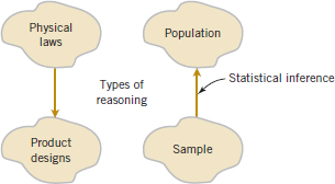
FIGURE 1-4 Statistical inference is one type of reasoning.

An effective data-collection procedure can greatly simplify the analysis and lead to improved understanding of the population or process that is being studied. We now consider some examples of these data-collection methods.

1-2.2 RETROSPECTIVE STUDY

Montgomery, Peck, and Vining (2012) describe an acetone-butyl alcohol distillation column for which concentration of acetone in the distillate (the output product stream) is an important variable. Factors that may affect the distillate are the reboil temperature, the condensate temperature, and the reflux rate. Production personnel obtain and archive the following records:

• The concentration of acetone in an hourly test sample of output product
• The reboil temperature log, which is a record of the reboil temperature over time
• The condenser temperature controller log
• The nominal reflux rate each hour

The reflux rate should be held constant for this process. Consequently, production personnel change this very infrequently.

A retrospective study would use either all or a sample of the historical process data archived over some period of time. The study objective might be to discover the relationships among the two temperatures and the reflux rate on the acetone concentration in the output product stream. However, this type of study presents some problems:

1. We may not be able to see the relationship between the reflux rate and acetone concentration because the reflux rate did not change much over the historical period.
2. The archived data on the two temperatures (which are recorded almost continuously) do not correspond perfectly to the acetone concentration measurements (which are made hourly). It may not be obvious how to construct an approximate correspondence.
3. Production maintains the two temperatures as closely as possible to desired targets or set points. Because the temperatures change so little, it may be difficult to assess their real impact on acetone concentration.
4. In the narrow ranges within which they do vary, the condensate temperature tends to increase with the reboil temperature. Consequently, the effects of these two process variables on acetone concentration may be difficult to separate.

As you can see, a retrospective study may involve a significant amount of data, but those data may contain relatively little useful information about the problem. Furthermore, some of the relevant data may be missing, there may be transcription or recording errors resulting in outliers (or unusual values), or data on other important factors may not have been collected and archived. In the distillation column, for example, the specific concentrations of butyl alcohol and acetone in the input feed stream are very important factors, but they are not archived because the concentrations are too hard to obtain on a routine basis. As a result of these types of issues, statistical analysis of historical data sometimes identifies interesting phenomena, but solid and reliable explanations of these phenomena are often difficult to obtain.

1-2.3 OBSERVATIONAL STUDY

In an observational study, the engineer observes the process or population, disturbing it as little as possible, and records the quantities of interest. Because these studies are usually conducted for a relatively short time period, sometimes variables that are not routinely measured can be included. In the distillation column, the engineer would design a form to record the two temperatures and the reflux rate when acetone concentration measurements are made. It may even be possible to measure the input feed stream concentrations so that the impact of this factor could be studied.

Generally, an observational study tends to solve problems 1 and 2 and goes a long way toward obtaining accurate and reliable data. However, observational studies may not help resolve problems 3 and 4.

1-2.4 DESIGNED EXPERIMENTS

In a designed experiment, the engineer makes deliberate or purposeful changes in the controllable variables of the system or process, observes the resulting system output data, and then makes an inference or decision about which variables are responsible for the observed changes in output performance. The nylon connector example in Section 1-1 illustrates a designed experiment; that is, a deliberate change was made in the connector's wall thickness with the objective of discovering whether or not a stronger pull-off force could be obtained. Experiments designed with basic principles such as randomization are needed to establish cause-and-effect relationships.

Much of what we know in the engineering and physical-chemical sciences is developed through testing or experimentation. Often engineers work in problem areas in which no scientific or engineering theory is directly or completely applicable, so experimentation and observation of the resulting data constitute the only way that the problem can be solved. Even when there is a good underlying scientific theory that we may rely on to explain the phenomena of interest, it is almost always necessary to conduct tests or experiments to confirm that the theory is indeed operative in the situation or environment in which it is being applied. Statistical thinking and statistical methods play an important role in planning, conducting, and analyzing the data from engineering experiments. Designed experiments play a very important role in engineering design and development and in the improvement of manufacturing processes.

For example, consider the problem involving the choice of wall thickness for the nylon connector. This is a simple illustration of a designed experiment. The engineer chose two wall thicknesses for the connector and performed a series of tests to obtain pull-off force measurements at each wall thickness. In this simple comparative experiment, the engineer is interested in determining whether there is any difference between the 3/32- and 1/8-inch designs. An approach that could be used in analyzing the data from this experiment is to compare the mean pull-off force for the 3/32-inch design to the mean pull-off force for the 1/8-inch design using statistical hypothesis testing, which is discussed in detail in Chapters 9 and 10. Generally, a hypothesis is a statement about some aspect of the system in which we are interested. For example, the engineer might want to know if the mean pull-off force of a 3/32-inch design exceeds the typical maximum load expected to be encountered in this application, say, 12.75 pounds. Thus, we would be interested in testing the hypothesis that the mean strength exceeds 12.75 pounds. This is called a single-sample hypothesis-testing problem. Chapter 9 presents techniques for this type of problem. Alternatively, the engineer might be interested in testing the hypothesis that increasing the wall thickness from 3/32 to 1/8 inch results in an increase in mean pull-off force. It is an example of a two-sample hypothesis-testing problem. Two-sample hypothesis-testing problems are discussed in Chapter 10.

Designed experiments offer a very powerful approach to studying complex systems, such as the distillation column. This process has three factors—the two temperatures and the reflux rate—and we want to investigate the effect of these three factors on output acetone concentration. A good experimental design for this problem must ensure that we can separate the effects of all three factors on the acetone concentration. The specified values of the three factors used in the experiment are called factor levels. Typically, we use a small number of levels such as two or three for each factor. For the distillation column problem, suppose that we use two levels, “high” and “low” (denoted +1 and −1, respectively), for each of the three factors. A very reasonable experiment design strategy uses every possible combination of the factor levels to form a basic experiment with eight different settings for the process. This type of experiment is called a factorial experiment. See Table 1-1 for this experimental design.

Figure 1-5 illustrates that this design forms a cube in terms of these high and low levels. With each setting of the process conditions, we allow the column to reach equilibrium, take a sample of the product stream, and determine the acetone concentration. We then can draw specific inferences about the effect of these factors. Such an approach allows us to proactively study a population or process.

TABLE • 1-1 The Designed Experiment (Factorial Design) for the Distillation Column

An important advantage of factorial experiments is that they allow one to detect an interaction between factors. Consider only the two temperature factors in the distillation experiment. Suppose that the response concentration is poor when the reboil temperature is low, regardless of the condensate temperature. That is, the condensate temperature has no effect when the reboil temperature is low. However, when the reboil temperature is high, a high condensate temperature generates a good response, but a low condensate temperature generates a poor response. That is, the condensate temperature changes the response when the reboil temperature is high. The effect of condensate temperature depends on the setting of the reboil temperature, and these two factors are said to interact in this case. If the four combinations of high and low reboil and condensate temperatures were not tested, such an interaction would not be detected.

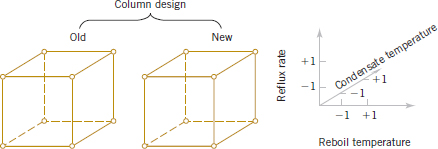
We can easily extend the factorial strategy to more factors. Suppose that the engineer wants to consider a fourth factor, type of distillation column. There are two types: the standard one and a newer design. Figure 1-6 illustrates how all four factors—reboil temperature, condensate temperature, reflux rate, and column design—could be investigated in a factorial design. Because all four factors are still at two levels, the experimental design can still be represented geometrically as a cube (actually, it's a hypercube). Notice that as in any factorial design, all possible combinations of the four factors are tested. The experiment requires 16 trials.

Generally, if there are k factors and each has two levels, a factorial experimental design will require 2^k runs. For example, with k = 4, the 2⁴ design in Fig. 1-6 requires 16 tests. Clearly, as the number of factors increases, the number of trials required in a factorial experiment increases rapidly; for instance, eight factors each at two levels would require 256 trials. This quickly becomes unfeasible from the viewpoint of time and other resources. Fortunately, with four to five or more factors, it is usually unnecessary to test all possible combinations of factor levels. A fractional factorial experiment is a variation of the basic factorial arrangement in which only a subset of the factor combinations is actually tested. Figure 1-7 shows a fractional factorial experimental design for the four-factor version of the distillation experiment. The circled test combinations in this figure are the only test combinations that need to be run. This experimental design requires only 8 runs instead of the original 16; consequently it would be called a one-half fraction. This is an excellent experimental design in which to study all four factors. It will provide good information about the individual effects of the four factors and some information about how these factors interact.

FIGURE 1-5 The factorial design for the distillation column.

FIGURE 1-6 A four-factorial experiment for the distillation column.

Factorial and fractional factorial experiments are used extensively by engineers and scientists in industrial research and development, where new technology, products, and processes are designed and developed and where existing products and processes are improved. Since so much engineering work involves testing and experimentation, it is essential that all engineers understand the basic principles of planning efficient and effective experiments. We discuss these principles in Chapter 13. Chapter 14 concentrates on the factorial and fractional factorials that we have introduced here.

1-2.5 Observing Processes Over Time

Often data are collected over time. In this case, it is usually very helpful to plot the data versus time in a time series plot. Phenomena that might affect the system or process often become more visible in a time-oriented plot and the concept of stability can be better judged.

Figure 1-8 is a dot diagram of acetone concentration readings taken hourly from the distillation column described in Section 1-2.2. The large variation displayed on the dot diagram indicates considerable variability in the concentration, but the chart does not help explain the reason for the variation. The time series plot is shown in Fig. 1-9. A shift in the process mean level is visible in the plot and an estimate of the time of the shift can be obtained.

W. Edwards Deming, a very influential industrial statistician, stressed that it is important to understand the nature of variability in processes and systems over time. He conducted an experiment in which he attempted to drop marbles as close as possible to a target on a table. He used a funnel mounted on a ring stand and the marbles were dropped into the funnel. See Fig. 1-10. The funnel was aligned as closely as possible with the center of the target. He then used two different strategies to operate the process. (1) He never moved the funnel. He just dropped one marble after another and recorded the distance from the target. (2) He dropped the first marble and recorded its location relative to the target. He then moved the funnel an equal and opposite distance in an attempt to compensate for the error. He continued to make this type of adjustment after each marble was dropped.

After both strategies were completed, he noticed that the variability of the distance from the target for strategy 2 was approximately twice as large than for strategy 1. The adjustments to the funnel increased the deviations from the target. The explanation is that the error (the deviation of the marble's position from the target) for one marble provides no information about the error that will occur for the next marble. Consequently, adjustments to the funnel do not decrease future errors. Instead, they tend to move the funnel farther from the target.

FIGURE 1-7 A fractional factorial experiment for the connector wall thickness problem.

FIGURE 1-8 The dot diagram illustrates variation but does not identify the problem.

FIGURE 1-9 A time series plot of concentration provides more information than the dot diagram.

This interesting experiment points out that adjustments to a process based on random disturbances can actually increase the variation of the process. This is referred to as overcontrol or tampering. Adjustments should be applied only to compensate for a nonrandom shift in the process—then they can help. A computer simulation can be used to demonstrate the lessons of the funnel experiment. Figure 1-11 displays a time plot of 100 measurements (denoted as y) from a process in which only random disturbances are present. The target value for the process is 10 units. The figure displays the data with and without adjustments that are applied to the process mean in an attempt to produce data closer to target. Each adjustment is equal and opposite to the deviation of the previous measurement from target. For example, when the measurement is 11 (one unit above target), the mean is reduced by one unit before the next measurement is generated. The overcontrol increases the deviations from the target.

Figure 1-12 displays the data without adjustment from Fig. 1-11, except that the measurements after observation number 50 are increased by two units to simulate the effect of a shift in the mean of the process. When there is a true shift in the mean of a process, an adjustment can be useful. Figure 1-12 also displays the data obtained when one adjustment (a decrease of two units) is applied to the mean after the shift is detected (at observation number 57). Note that this adjustment decreases the deviations from target.

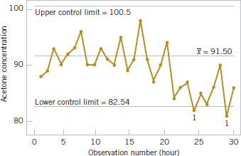
The question of when to apply adjustments (and by what amounts) begins with an understanding of the types of variation that affect a process. The use of a control charts is an invaluable way to examine the variability in time-oriented data. Figure 1-13 presents a control chart for the concentration data from Fig. 1-9. The center line on the control chart is just the average of the concentration measurements for the first 20 samples ( = 91.5 g/l) when the process is stable. The upper control limit and the lower control limit are a pair of statistically derived limits that reflect the inherent or natural variability in the process. These limits are located 3 standard deviations of the concentration values above and below the center line. If the process is operating as it should without any external sources of variability present in the system, the concentration measurements should fluctuate randomly around the center line, and almost all of them should fall between the control limits.

In the control chart of Fig. 1-13, the visual frame of reference provided by the center line and the control limits indicates that some upset or disturbance has affected the process around sample 20 because all of the following observations are below the center line, and two of them actually fall below the lower control limit. This is a very strong signal that corrective action is required in this process. If we can find and eliminate the underlying cause of this upset, we can improve process performance considerably. Thus control limits serve as decision rules about actions that could be taken to improve the process.

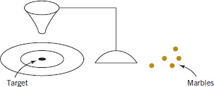
FIGURE 1-10 Deming's funnel experiment.

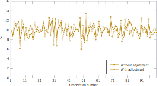
FIGURE 1-11 Adjustments applied to random disturbances overcontrol the process and increase the deviations from the target.

Furthermore, Deming pointed out that data from a process are used for different types of conclusions. Sometimes we collect data from a process to evaluate current production. For example, we might sample and measure resistivity on three semiconductor wafers selected from a lot and use this information to evaluate the lot. This is called an enumerative study. However, in many cases, we use data from current production to evaluate future production. We apply conclusions to a conceptual, future population. Deming called this an analytic study. Clearly this requires an assumption of a stable process, and Deming emphasized that control charts were needed to justify this assumption. See Fig. 1-14 as an illustration.

The use of control charts is a very important application of statistics for monitoring, controlling, and improving a process. The branch of statistics that makes use of control charts is called statistical process control, or SPC. We will discuss SPC and control charts in Chapter 15.

FIGURE 1-12 Process mean shift is detected at observation number 57, and one adjustment (a decrease of two units) reduces the deviations from target.

FIGURE 1-13 A control chart for the chemical process concentration data.

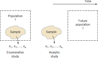
FIGURE 1-14 Enumerative versus analytic study.

1-3 Mechanistic and Empirical Models

Models play an important role in the analysis of nearly all engineering problems. Much of the formal education of engineers involves learning about the models relevant to specific fields and the techniques for applying these models in problem formulation and solution. As a simple example, suppose that we are measuring the flow of current in a thin copper wire. Our model for this phenomenon might be Ohm's law:

We call this type of model a mechanistic model because it is built from our underlying knowledge of the basic physical mechanism that relates these variables. However, if we performed this measurement process more than once, perhaps at different times, or even on different days, the observed current could differ slightly because of small changes or variations in factors that are not completely controlled, such as changes in ambient temperature, fluctuations in performance of the gauge, small impurities present at different locations in the wire, and drifts in the voltage source. Consequently, a more realistic model of the observed current might be

where is a term added to the model to account for the fact that the observed values of current flow do not perfectly conform to the mechanistic model. We can think of as a term that includes the effects of all unmodeled sources of variability that affect this system.

Sometimes engineers work with problems for which no simple or well-understood mechanistic model explains the phenomenon. For instance, suppose that we are interested in the number average molecular weight (M_n) of a polymer. Now we know that M_n is related to the viscosity of the material (V), and it also depends on the amount of catalyst (C) and the temperature (T) in the polymerization reactor when the material is manufactured. The relationship between M_n and these variables is

say, where the form of the function f is unknown. Perhaps a working model could be developed from a first-order Taylor series expansion, which would produce a model of the form

where the β's are unknown parameters. Now just as in Ohm's law, this model will not exactly describe the phenomenon, so we should account for the other sources of variability that may affect the molecular weight by adding another term to the model; therefore,

is the model that we will use to relate molecular weight to the other three variables. This type of model is called an empirical model; that is, it uses our engineering and scientific knowledge of the phenomenon, but it is not directly developed from our theoretical or first-principles understanding of the underlying mechanism.

To illustrate these ideas with a specific example, consider the data in Table 1-2, which contains data on three variables that were collected in an observational study in a semiconductor manufacturing plant. In this plant, the finished semiconductor is wire-bonded to a frame. The variables reported are pull strength (a measure of the amount of force required to break the bond), the wire length, and the height of the die. We would like to find a model relating pull strength to wire length and die height. Unfortunately, there is no physical mechanism that we can easily apply here, so it does not seem likely that a mechanistic modeling approach will be successful.

Figure 1-15 presents a three-dimensional plot of all 25 observations on pull strength, wire length, and die height. From examination of this plot, we see that pull strength increases as both wire length and die height increase. Furthermore, it seems reasonable to think that a model such as

would be appropriate as an empirical model for this relationship. In general, this type of empirical model is called a regression model. In Chapters 11 and 12 we show how to build these models and test their adequacy as approximating functions. We will use a method for estimating the parameters in regression models, called the method of least squares, that traces its origins to work by Karl Gauss. Essentially, this method chooses the parameters in the empirical model (the β's) to minimize the sum of the squared distances in each data point and the plane represented by the model equation. Applying this technique to the data in Table 1-2 results in

where the “hat,” or circumflex, over pull strength indicates that this is an estimated or predicted quality.

Figure 1-16 is a plot of the predicted values of pull strength versus wire length and die height obtained from Equation 1-7. Notice that the predicted values lie on a plane above the wire length–die height space. From the plot of the data in Fig. 1-15, this model does not appear unreasonable. The empirical model in Equation 1-7 could be used to predict values of pull strength for various combinations of wire length and die height that are of interest. Essentially, an engineer could use the empirical model in exactly the same way as a mechanistic model.

1-4 Probability and Probability Models

Section 1-1 mentioned that decisions often need to be based on measurements from only a subset of objects selected in a sample. This process of reasoning from a sample of objects to conclusions for a population of objects was referred to as statistical inference. A sample of three wafers selected from a large production lot of wafers in semiconductor manufacturing was an example mentioned. To make good decisions, an analysis of how well a sample represents a population is clearly necessary. If the lot contains defective wafers, how well will the sample detect these defective items? How can we quantify the criterion to “detect well?” Basically, how can we quantify the risks of decisions based on samples? Furthermore, how should samples be selected to provide good decisions—ones with acceptable risks? Probability models help quantify the risks involved in statistical inference, that is, the risks involved in decisions made every day.

FIGURE 1-15 Three-dimensional plot of the wire bond pull strength data.

TABLE • 1-2 Wire Bond Pull Strength Data

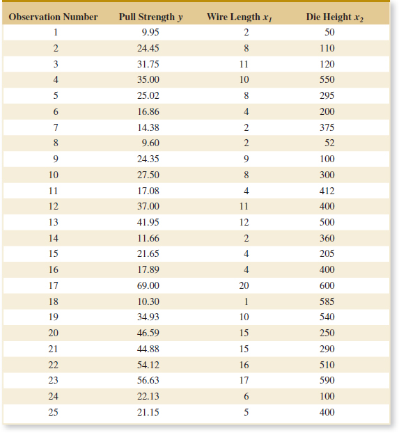
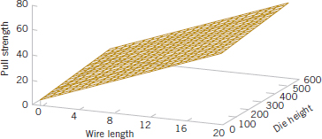
FIGURE 1-16 Plot of predicted values of pull strength from the empirical model.

More details are useful to describe the role of probability models. Suppose that a production lot contains 25 wafers. If all the wafers are defective or all are good, clearly any sample will generate all defective or all good wafers, respectively. However, suppose that only 1 wafer in the lot is defective. Then a sample might or might not detect (include) the wafer. A probability model, along with a method to select the sample, can be used to quantify the risks that the defective wafer is or is not detected. Based on this analysis, the size of the sample might be increased (or decreased). The risk here can be interpreted as follows. Suppose that a series of lots, each with exactly one defective wafer, is sampled. The details of the method used to select the sample are postponed until randomness is discussed in the next chapter. Nevertheless, assume that the same size sample (such as three wafers) is selected in the same manner from each lot. The proportion of the lots in which the defective wafer are included in the sample or, more specifically, the limit of this proportion as the number of lots in the series tends to infinity, is interpreted as the probability that the defective wafer is detected.

A probability model is used to calculate this proportion under reasonable assumptions for the manner in which the sample is selected. This is fortunate because we do not want to attempt to sample from an infinite series of lots. Problems of this type are worked in Chapters 2 and 3. More importantly, this probability provides valuable, quantitative information regarding any decision about lot quality based on the sample.

Recall from Section 1-1 that a population might be conceptual, as in an analytic study that applies statistical inference to future production based on the data from current production. When populations are extended in this manner, the role of statistical inference and the associated probability models become even more important.

In the previous example, each wafer in the sample was classified only as defective or not. Instead, a continuous measurement might be obtained from each wafer. In Section 1-2.5, concentration measurements were taken at periodic intervals from a production process. Figure 1-8 shows that variability is present in the measurements, and there might be concern that the process has moved from the target setting for concentration. Similar to the defective wafer, one might want to quantify our ability to detect a process change based on the sample data. Control limits were mentioned in Section 1-2.5 as decision rules for whether or not to adjust a process. The probability that a particular process change is detected can be calculated with a probability model for concentration measurements. Models for continuous measurements are developed based on plausible assumptions for the data and a result known as the central limit theorem, and the associated normal distribution is a particularly valuable probability model for statistical inference. Of course, a check of assumptions is important. These types of probability models are discussed in Chapter 4. The objective is still to quantify the risks inherent in the inference made from the sample data.

Throughout Chapters 6 through 15, we base decisions on statistical inference from sample data. We use continuous probability models, specifically the normal distribution, extensively to quantify the risks in these decisions and to evaluate ways to collect the data and how large a sample should be selected.

Important Terms and Concepts

Analytic study

Cause and effect

Designed experiment

Empirical model

Engineering method

Enumerative study

Factorial experiment

Fractional factorial experiment

Hypothesis

Hypothesis testing

Interaction

Mechanistic model

Observational study

Overcontrol

Population

Probability model

Random variable

Randomization

Retrospective study

Sample

Scientific method

Statistical inference

Statistical process control

Statistical thinking

Tampering

Time series

Variability