

Point Estimation of Parameters and Sampling Distributions

Chapter Outline
7-2 Sampling Distributions and the Central Limit Theorem
7-3 General Concepts of Point Estimation
7-3.2 Variance of a Point Estimator
7-3.3 Standard Error: Reporting a Point Estimate
7-3.4 Bootstrap Standard Error
7-3.5 Mean Squared Error of an Estimator
7-4 Methods of Point Estimation
Introduction
Statistical methods are used to make decisions and draw conclusions about populations. This aspect of statistics is generally called statistical inference. These techniques utilize the information in a sample for drawing conclusions. This chapter begins our study of the statistical methods used in decision making.
Statistical inference may be divided into two major areas: parameter estimation and hypothesis testing. As an example of a parameter estimation problem, suppose that an engineer is analyzing the tensile strength of a component used in an air frame. This is an important part of assessing the overall structural integrity of the airplane. Variability is naturally present in the individual components because of differences in the batches of raw material used to make the components, manufacturing processes, and measurement procedures (for example), so the engineer wants to estimate the mean strength of the population of components. In practice, the engineer will use sample data to compute a number that is in some sense a reasonable value (a good guess) of the true population mean. This number is called a point estimate. We will see that procedures are available for developing point estimates of parameters that have good statistical properties. We will also be able to establish the precision of the point estimate.
Now let's consider a different type of question. Suppose that two different reaction temperatures t1 and t2 can be used in a chemical process. The engineer conjectures that t1 will result in higher yields than t2. If the engineers can demonstrate that t1 results in higher yields, then a process change can probably be justified. Statistical hypothesis testing is the framework for solving problems of this type. In this example, the engineer would be interested in formulating hypotheses that allow him or her to demonstrate that the mean yield using t1 is higher than the mean yield using t2. Notice that there is no emphasis on estimating yields; instead, the focus is on drawing conclusions about a hypothesis that is relevant to the engineering decision.
This chapter and Chapter 8 discuss parameter estimation. Chapters 9 and 10 focus on hypothesis testing.
![]() Learning Objectives
Learning Objectives
After careful study of this chapter, you should be able to do the following:
- Explain the general concepts of estimating the parameters of a population or a probability distribution
- Explain the important role of the normal distribution as a sampling distribution
- Understand the central limit theorem
- Explain important properties of point estimators, including bias, variance, and mean square error
- Know how to construct point estimators using the method of moments and the method of maximum likelihood
- Know how to compute and explain the precision with which a parameter is estimated
- Know how to construct a point estimator using the Bayesian approach
7-1 Point Estimation
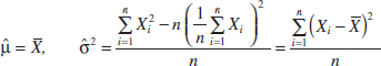
Statistical inference always focuses on drawing conclusions about one or more parameters of a population. An important part of this process is obtaining estimates of the parameters. Suppose that we want to obtain a point estimate (a reasonable value) of a population parameter. We know that before the data are collected, the observations are considered to be random variables, say, X1, X2,..., Xn. Therefore, any function of the observation, or any statistic, is also a random variable. For example, the sample mean ![]() and the sample variance S2 are statistics and random variables.
and the sample variance S2 are statistics and random variables.
Another way to visualize this is as follows. Suppose we take a sample of n = 10 observations from a population and compute the sample average, getting the result ![]() = 10.2. Now we repeat this process, taking a second sample of n = 10 observations from the same population and the resulting sample average is 10.4. The sample average depends on the observations in the sample, which differ from sample to sample because they are random variables. Consequently, the sample average (or any other function of the sample data) is a random variable.
= 10.2. Now we repeat this process, taking a second sample of n = 10 observations from the same population and the resulting sample average is 10.4. The sample average depends on the observations in the sample, which differ from sample to sample because they are random variables. Consequently, the sample average (or any other function of the sample data) is a random variable.
Because a statistic is a random variable, it has a probability distribution. We call the probability distribution of a statistic a sampling distribution. The notion of a sampling distribution is very important and will be discussed and illustrated later in the chapter.
When discussing inference problems, it is convenient to have a general symbol to represent the parameter of interest. We will use the Greek symbol θ (theta) to represent the parameter. The symbol θ can represent the mean μ, the variance σ2, or any parameter of interest to us. The objective of point estimation is to select a single number based on sample data that is the most plausible value for θ. A numerical value of a sample statistic will be used as the point estimate.
In general, if X is a random variable with probability distribution f(x), characterized by the unknown parameter θ, and if X1, X2,..., Xn is a random sample of size n from X, the statistic ![]() = h(X1, X2,..., Xn) is called a point estimator of θ. Note that
= h(X1, X2,..., Xn) is called a point estimator of θ. Note that ![]() is a random variable because it is a function of random variables. After the sample has been selected,
is a random variable because it is a function of random variables. After the sample has been selected, ![]() takes on a particular numerical value
takes on a particular numerical value ![]() called the point estimate of θ.
called the point estimate of θ.
Point Estimator
A point estimate of some population parameter θ is a single numerical value ![]() of a statistic
of a statistic ![]() . The statistic
. The statistic ![]() is called the point estimator.
is called the point estimator.
As an example, suppose that the random variable X is normally distributed with an unknown mean μ. The sample mean is a point estimator of the unknown population mean μ. That is, ![]() =
= ![]() . After the sample has been selected, the numerical value
. After the sample has been selected, the numerical value ![]() is the point estimate of μ. Thus, if x1 = 25, x2 = 30, x3 = 29, and x4 = 31, the point estimate of μ is
is the point estimate of μ. Thus, if x1 = 25, x2 = 30, x3 = 29, and x4 = 31, the point estimate of μ is
![]()
Similarly, if the population variance σ2 is also unknown, a point estimator for σ2 is the sample variance S2, and the numerical value s2 = 6.9 calculated from the sample data is called the point estimate of σ2.
Estimation problems occur frequently in engineering. We often need to estimate
- The mean μ of a single population
- The variance σ2 (or standard deviation σ) of a single population
- The proportion p of items in a population that belong to a class of interest
- The difference in means of two populations, μ1 − μ2
- The difference in two population proportions, p1 − p2
Reasonable point estimates of these parameters are as follows:
- For μ, the estimate is
 =
=  , the sample mean.
 - For σ2, the estimate is
 2 = s2, the sample variance.
 - For p, the estimate is
 = x/n, the sample proportion, where x is the number of items in a random sample of size n that belong to the class of interest.
 - For μ1 − μ2, the estimate is 1 − 2 = 1 − 2, the difference between the sample means of two independent random samples.
- For p1 − p2, the estimate is 1 − 2, the difference between two sample proportions computed from two independent random samples.
We may have several different choices for the point estimator of a parameter. For example, if we wish to estimate the mean of a population, we might consider the sample mean, the sample median, or perhaps the average of the smallest and largest observations in the sample as point estimators. To decide which point estimator of a particular parameter is the best one to use, we need to examine their statistical properties and develop some criteria for comparing estimators.
7-2 Sampling Distributions and the Central Limit Theorem
Statistical inference is concerned with making decisions about a population based on the information contained in a random sample from that population. For instance, we may be interested in the mean fill volume of a container of soft drink. The mean fill volume in the population is required to be 300 milliliters. An engineer takes a random sample of 25 containers and computes the sample average fill volume to be ![]() = 298.8 milliliters. The engineer will probably decide that the population mean is μ = 300 milliliters even though the sample mean was 298.8 milliliters because he or she knows that the sample mean is a reasonable estimate of μ and that a sample mean of 298.8 milliliters is very likely to occur even if the true population mean is μ = 300 milliliters. In fact, if the true mean is 300 milliliters, tests of 25 containers made repeatedly, perhaps every five minutes, would produce values of
= 298.8 milliliters. The engineer will probably decide that the population mean is μ = 300 milliliters even though the sample mean was 298.8 milliliters because he or she knows that the sample mean is a reasonable estimate of μ and that a sample mean of 298.8 milliliters is very likely to occur even if the true population mean is μ = 300 milliliters. In fact, if the true mean is 300 milliliters, tests of 25 containers made repeatedly, perhaps every five minutes, would produce values of ![]() that vary both above and below μ = 300 milliliters.
that vary both above and below μ = 300 milliliters.
The link between the probability models in the earlier chapters and the data is made as follows. Each numerical value in the data is the observed value of a random variable. Furthermore, the random variables are usually assumed to be independent and identically distributed. These random variables are known as a random sample.
Random Sample
The random variables X1, X2,..., Xn are a random sample of size n if (a) the Xi's are independent random variables and (b) every Xi has the same probability distribution.
The observed data are also referred to as a random sample, but the use of the same phrase should not cause any confusion.
The assumption of a random sample is extremely important. If the sample is not random and is based on judgment or is flawed in some other way, statistical methods will not work properly and will lead to incorrect decisions.
The primary purpose in taking a random sample is to obtain information about the unknown population parameters. Suppose, for example, that we wish to reach a conclusion about the proportion of people in the United States who prefer a particular brand of soft drink. Let p represent the unknown value of this proportion. It is impractical to question every individual in the population to determine the true value of p. To make an inference regarding the true proportion p, a more reasonable procedure would be to select a random sample (of an appropriate size) and use the observed proportion ![]() of people in this sample favoring the brand of soft drink.
of people in this sample favoring the brand of soft drink.
The sample proportion, ![]() , is computed by dividing the number of individuals in the sample who prefer the brand of soft drink by the total sample size n. Thus,
, is computed by dividing the number of individuals in the sample who prefer the brand of soft drink by the total sample size n. Thus, ![]() is a function of the observed values in the random sample. Because many random samples are possible from a population, the value of
is a function of the observed values in the random sample. Because many random samples are possible from a population, the value of ![]() will vary from sample to sample. That is,
will vary from sample to sample. That is, ![]() is a random variable. Such a random variable is called a statistic.
is a random variable. Such a random variable is called a statistic.
Statistic
A statistic is any function of the observations in a random sample.
We have encountered statistics before. For example, if X, X2,..., Xn is a random sample of size n, the sample mean ![]() , the sample variance S2, and the sample standard deviation S are statistics. Because a statistic is a random variable, it has a probability distribution.
, the sample variance S2, and the sample standard deviation S are statistics. Because a statistic is a random variable, it has a probability distribution.
Sampling Distribution
The probability distribution of a statistic is called a sampling distribution.
For example, the probability distribution of ![]() is called the sampling distribution of the mean. The sampling distribution of a statistic depends on the distribution of the population, the size of the sample, and the method of sample selection. We now present perhaps the most important sampling distribution. Other sampling distributions and their applications will be illustrated extensively in the following two chapters.
is called the sampling distribution of the mean. The sampling distribution of a statistic depends on the distribution of the population, the size of the sample, and the method of sample selection. We now present perhaps the most important sampling distribution. Other sampling distributions and their applications will be illustrated extensively in the following two chapters.
Consider determining the sampling distribution of the sample mean ![]() . Suppose that a random sample of size n is taken from a normal population with mean μ and variance σ2. Now each observation in this sample, say, X1, X2,..., Xn, is a normally and independently distributed random variable with mean μ and variance σ2. Then because linear functions of independent, normally distributed random variables are also normally distributed (Chapter 5), we conclude that the sample mean
. Suppose that a random sample of size n is taken from a normal population with mean μ and variance σ2. Now each observation in this sample, say, X1, X2,..., Xn, is a normally and independently distributed random variable with mean μ and variance σ2. Then because linear functions of independent, normally distributed random variables are also normally distributed (Chapter 5), we conclude that the sample mean
![]()
has a normal distribution with mean
![]()
and variance
![]()
If we are sampling from a population that has an unknown probability distribution, the sampling distribution of the sample mean will still be approximately normal with mean μ and variance σ2/n if the sample size n is large. This is one of the most useful theorems in statistics, called the central limit theorem. The statement is as follows:
Central Limit Theorem
If X1, X2,..., Xn is a random sample of size n taken from a population (either finite or infinite) with mean μ and finite variance σ2 and if ![]() is the sample mean, the limiting form of the distribution of
is the sample mean, the limiting form of the distribution of
![]()
as n → ∞, is the standard normal distribution.
It is easy to demonstrate the central limit theorem with a computer simulation experiment. Consider the lognormal distribution in Fig. 7-1. This distribution has parameters θ = 2 (called the location parameter) and ω = 0.75 (called the scale parameter), resulting in mean μ = 9.79 and standard deviation σ = 8.51. Notice that this lognormal distribution does not look very much like the normal distribution; it is defined only for positive values of the random variable X and is skewed considerably to the right. We used computer software to draw 20 samples at random from this distribution, each of size n = 10. The data from this sampling experiment are shown in Table 7-1. The last row in this table is the average of each sample ![]() .
.
The first thing that we notice in looking at the values of ![]() is that they are not all the same. This is a clear demonstration of the point made previously that any statistic is a random variable. If we had calculated any sample statistic (s, the sample median, the upper or lower quartile, or a percentile), they would also have varied from sample to sample because they are random variables. Try it and see for yourself.
is that they are not all the same. This is a clear demonstration of the point made previously that any statistic is a random variable. If we had calculated any sample statistic (s, the sample median, the upper or lower quartile, or a percentile), they would also have varied from sample to sample because they are random variables. Try it and see for yourself.

FIGURE 7-1 A lognormal distribution with θ = 2 and ω = 0.75.
According to the central limit theorem, the distribution of the sample average ![]() is normal. Figure 7-2 is a normal probability plot of the 20 sample averages
is normal. Figure 7-2 is a normal probability plot of the 20 sample averages ![]() from Table 7-1. The observations scatter generally along a straight line, providing evidence that the distribution of the sample mean is normal even though the distribution of the population is very non-normal. This type of sampling experiment can be used to investigate the sampling distribution of any statistic.
from Table 7-1. The observations scatter generally along a straight line, providing evidence that the distribution of the sample mean is normal even though the distribution of the population is very non-normal. This type of sampling experiment can be used to investigate the sampling distribution of any statistic.
The normal approximation for ![]() depends on the sample size n. Figure 7-3(a) is the distribution obtained for throws of a single, six-sided true die. The probabilities are equal (1/6) for all the values obtained: 1, 2, 3, 4, 5, or 6. Figure 7-3(b) is the distribution of the average score obtained when tossing two dice, and Fig. 7-3(c), 7-3(d), and 7-3(e) show the distributions of average scores obtained when tossing 3, 5, and 10 dice, respectively. Notice that, although the population (one die) is relatively far from normal, the distribution of averages is approximated reasonably well by the normal distribution for sample sizes as small as five. (The dice throw distributions are discrete, but the normal is continuous.)
depends on the sample size n. Figure 7-3(a) is the distribution obtained for throws of a single, six-sided true die. The probabilities are equal (1/6) for all the values obtained: 1, 2, 3, 4, 5, or 6. Figure 7-3(b) is the distribution of the average score obtained when tossing two dice, and Fig. 7-3(c), 7-3(d), and 7-3(e) show the distributions of average scores obtained when tossing 3, 5, and 10 dice, respectively. Notice that, although the population (one die) is relatively far from normal, the distribution of averages is approximated reasonably well by the normal distribution for sample sizes as small as five. (The dice throw distributions are discrete, but the normal is continuous.)
The central limit theorem is the underlying reason why many of the random variables encountered in engineering and science are normally distributed. The observed variable of the results from a series of underlying disturbances that act together to create a central limit effect.
![]() TABLE • 7-1 Twenty samples of size n = 10 from the lognormal distribution in Figure 7-1.
TABLE • 7-1 Twenty samples of size n = 10 from the lognormal distribution in Figure 7-1.


FIGURE 7-2 Normal probability plot of the sample averages from Table 7-1.

FIGURE 7-3 Distributions of average scores from throwing dice.
Source: [Adapted with permission from Box, Hunter, and Hunter (1978).]
When is the sample size large enough so that the central limit theorem can be assumed to apply? The answer depends on how close the underlying distribution is to the normal. If the underlying distribution is symmetric and unimodal (not too far from normal), the central limit theorem will apply for small values of n, say 4 or 5. If the sampled population is very non-normal, larger samples will be required. As a general guideline, if n > 30, the central limit theorem will almost always apply. There are exceptions to this guideline are relatively rare. In most cases encountered in practice, this guideline is very conservative, and the central limit theorem will apply for sample sizes much smaller than 30. For example, consider the dice example in Fig. 7-3.
Example 7-1 Resistors An electronics company manufactures resistors that have a mean resistance of 100 ohms and a standard deviation of 10 ohms. The distribution of resistance is normal. Find the probability that a random sample of n = 25 resistors will have an average resistance of fewer than 95 ohms.
Note that the sampling distribution of ![]() is normal with mean
is normal with mean ![]() = 100 ohms and a standard deviation of
= 100 ohms and a standard deviation of
![]()
Therefore, the desired probability corresponds to the shaded area in Fig. 7-4. Standardizing the point ![]() = 95 in Fig. 7-4, we find that
= 95 in Fig. 7-4, we find that
and therefore,
![]()
Practical Conclusion: This example shows that if the distribution of resistance is normal with mean 100 ohms and standard deviation of 10 ohms, finding a random sample of resistors with a sample mean less than 95 ohms is a rare event. If this actually happens, it casts doubt as to whether the true mean is really 100 ohms or if the true standard deviation is really 10 ohms.
The following example makes use of the central limit theorem.
Example 7-2 Central Limit Theorem Suppose that a random variable X has a continuous uniform distribution
![]()
Find the distribution of the sample mean of a random sample of size n = 40.
The mean and variance of X are μ = 5 and σ2 = (6 − 4)2/12 = 1/3. The central limit theorem indicates that the distribution of ![]() is approximately normal with mean
is approximately normal with mean ![]() = 5 and variance
= 5 and variance ![]() = σ2/n = 1/[3(40)] = 1/120. See the distributions of X and
= σ2/n = 1/[3(40)] = 1/120. See the distributions of X and ![]() in Fig. 7-5.
in Fig. 7-5.
Now consider the case in which we have two independent populations. Let the first population have mean μ1 and variance ![]() and the second population have mean μ2 and variance
and the second population have mean μ2 and variance ![]() . Suppose that both populations are normally distributed. Then, using the fact that linear combinations of independent normal random variables follow a normal distribution (see Chapter 5), we can say that the sampling distribution of
. Suppose that both populations are normally distributed. Then, using the fact that linear combinations of independent normal random variables follow a normal distribution (see Chapter 5), we can say that the sampling distribution of ![]() 1 −
1 − ![]() 2 is normal with mean
2 is normal with mean
![]()
and variance
![]()
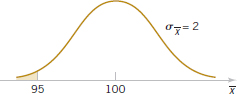
FIGURE 7-4 Probability for Example 7-1.
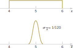
FIGURE 7-5 The distribution of X and ![]() for Example 7-2.
for Example 7-2.
If the two populations are not normally distributed and if both sample sizes n1 and n2 are more than 30, we may use the central limit theorem and assume that ![]() 2 and
2 and ![]() 2 follow approximately independent normal distributions. Therefore, the sampling distribution of
2 follow approximately independent normal distributions. Therefore, the sampling distribution of ![]() 1 −
1 − ![]() 2 is approximately normal with mean and variance given by Equations 7-2 and 7-3, respectively. If either n1 or n2 is fewer than 30, the sampling distribution of
2 is approximately normal with mean and variance given by Equations 7-2 and 7-3, respectively. If either n1 or n2 is fewer than 30, the sampling distribution of ![]() 1 −
1 − ![]() 2 will still be approximately normal with mean and variance given by Equations 7-2 and 7-3 provided that the population from which the small sample is taken is not dramatically different from the normal. We may summarize this with the following definition.
2 will still be approximately normal with mean and variance given by Equations 7-2 and 7-3 provided that the population from which the small sample is taken is not dramatically different from the normal. We may summarize this with the following definition.
Approximate Sampling Distribution of a Difference in Sample Means
If we have two independent populations with means μ1 and μ2 and variances ![]() and
and ![]() and if
and if ![]() 1 and
1 and ![]() 2 are the sample means of two independent random samples of sizes n1 and n2 from these populations, then the sampling distribution of
2 are the sample means of two independent random samples of sizes n1 and n2 from these populations, then the sampling distribution of
![]()
is approximately standard normal if the conditions of the central limit theorem apply. If the two populations are normal, the sampling distribution of Z is exactly standard normal.
Example 7-3 Aircraft Engine Life The effective life of a component used in a jet-turbine aircraft engine is a random variable with mean 5000 hours and standard deviation 40 hours. The distribution of effective life is fairly close to a normal distribution. The engine manufacturer introduces an improvement into the manufacturing process for this component that increases the mean life to 5050 hours and decreases the standard deviation to 30 hours. Suppose that a random sample of n1 = 16 components is selected from the “old” process and a random sample of n2 = 25 components is selected from the “improved” process. What is the probability that the difference in the two samples means ![]() 2 −
2 − ![]() 1 is at least 25 hours? Assume that the old and improved processes can be regarded as independent populations.
1 is at least 25 hours? Assume that the old and improved processes can be regarded as independent populations.
To solve this problem, we first note that the distribution of ![]() 1 is normal with mean μ1 = 5000 hours and standard deviation
1 is normal with mean μ1 = 5000 hours and standard deviation ![]() hours, and the distribution of
hours, and the distribution of ![]() 2 is normal with mean μ2 = 5050 hours and standard deviation
2 is normal with mean μ2 = 5050 hours and standard deviation ![]() hours. Now the distribution of
hours. Now the distribution of ![]() 2 −
2 − ![]() 1 is normal with mean μ2 − μ1 = 5050 − 5000 = 50 hours and variance
1 is normal with mean μ2 − μ1 = 5050 − 5000 = 50 hours and variance ![]() = (6)2 + (10)2 = 136 hours2. This sampling distribution is shown in Fig. 7-6. The probability that
= (6)2 + (10)2 = 136 hours2. This sampling distribution is shown in Fig. 7-6. The probability that ![]() 2 −
2 − ![]() 1 ≥ 25 is the shaded portion of the normal distribution in this figure.
1 ≥ 25 is the shaded portion of the normal distribution in this figure.
Corresponding to the value ![]() 2 −
2 − ![]() 1 = 25 in Fig. 7-4, we find that
1 = 25 in Fig. 7-4, we find that
![]()
and consequently,
![]()
Therefore, there is a high probability (0.9838) that the difference in sample means between the new and the old process will be at least 25 hours if the sample sizes are n1 = 16 and n2 = 25.

FIGURE 7-6 The sampling distribution of ![]() 2 −
2 − ![]() 1 in Example 7-3.
1 in Example 7-3.
![]() Problem available in WileyPLUS at instructor's discretion
Problem available in WileyPLUS at instructor's discretion
![]() Go Tutorial Tutoring problem available in WileyPLUS at instructor's discretion.
Go Tutorial Tutoring problem available in WileyPLUS at instructor's discretion.
7-1. Consider the hospital emergency room data from Exercise 6-124. Estimate the proportion of patients who arrive at this emergency department experiencing chest pain.
7-2. ![]() Consider the compressive strength data in Table 6-2. What proportion of the specimens exhibit compressive strength of at least 200 psi?
Consider the compressive strength data in Table 6-2. What proportion of the specimens exhibit compressive strength of at least 200 psi?
7-3. ![]() PVC pipe is manufactured with a mean diameter of 1.01 inch and a standard deviation of 0.003 inch. Find the probability that a random sample of n = 9 sections of pipe will have a sample mean diameter greater than 1.009 inch and less than 1.012 inch.
PVC pipe is manufactured with a mean diameter of 1.01 inch and a standard deviation of 0.003 inch. Find the probability that a random sample of n = 9 sections of pipe will have a sample mean diameter greater than 1.009 inch and less than 1.012 inch.
7-4. ![]() Suppose that samples of size n = 25 are selected at random from a normal population with mean 100 and standard deviation 10. What is the probability that the sample mean falls in the interval from
Suppose that samples of size n = 25 are selected at random from a normal population with mean 100 and standard deviation 10. What is the probability that the sample mean falls in the interval from ![]() to
to ![]() ?
?
7-5. ![]() A synthetic fiber used in manufacturing carpet has tensile strength that is normally distributed with mean 75.5 psi and standard deviation 3.5 psi. Find the probability that a random sample of n = 6 fiber specimens will have sample mean tensile strength that exceeds 75.75 psi.
A synthetic fiber used in manufacturing carpet has tensile strength that is normally distributed with mean 75.5 psi and standard deviation 3.5 psi. Find the probability that a random sample of n = 6 fiber specimens will have sample mean tensile strength that exceeds 75.75 psi.
7-6. ![]() Consider the synthetic fiber in the previous exercise. How is the standard deviation of the sample mean changed when the sample size is increased from n = 6 to n = 49?
Consider the synthetic fiber in the previous exercise. How is the standard deviation of the sample mean changed when the sample size is increased from n = 6 to n = 49?
7-7. ![]() The compressive strength of concrete is normally distributed with μ = 2500 psi and σ = 50 psi. Find the probability that a random sample of n = 5 specimens will have a sample mean diameter that falls in the interval from 2499 psi to 2510 psi.
The compressive strength of concrete is normally distributed with μ = 2500 psi and σ = 50 psi. Find the probability that a random sample of n = 5 specimens will have a sample mean diameter that falls in the interval from 2499 psi to 2510 psi.
7-8. ![]() Consider the concrete specimens in Exercise 7-7. What is the standard error of the sample mean?
Consider the concrete specimens in Exercise 7-7. What is the standard error of the sample mean?
7-9. ![]() A normal population has mean 100 and variance 25. How large must the random sample be if you want the standard error of the sample average to be 1.5?
A normal population has mean 100 and variance 25. How large must the random sample be if you want the standard error of the sample average to be 1.5?
7-10. ![]() Suppose that the random variable X has the continuous uniform distribution
Suppose that the random variable X has the continuous uniform distribution
![]()
Suppose that a random sample of n = 12 observations is selected from this distribution. What is the approximate probability distribution of ![]() − 6? Find the mean and variance of this quantity.
− 6? Find the mean and variance of this quantity.
7-11. ![]() Suppose that X has a discrete uniform distribution
Suppose that X has a discrete uniform distribution
![]()
A random sample of n = 36 is selected from this population. Find the probability that the sample mean is greater than 2.1 but less than 2.5, assuming that the sample mean would be measured to the nearest tenth.
7-12. ![]() The amount of time that a customer spends waiting at an airport check-in counter is a random variable with mean 8.2 minutes and standard deviation 1.5 minutes. Suppose that a random sample of n = 49 customers is observed. Find the probability that the average time waiting in line for these customers is
The amount of time that a customer spends waiting at an airport check-in counter is a random variable with mean 8.2 minutes and standard deviation 1.5 minutes. Suppose that a random sample of n = 49 customers is observed. Find the probability that the average time waiting in line for these customers is
(a) Less than 10 minutes
(b) Between 5 and 10 minutes
(c) Less than 6 minutes
7-13. ![]() A random sample of size n1 = 16 is selected from a normal population with a mean of 75 and a standard deviation of 8. A second random sample of size n2 = 9 is taken from another normal population with mean 70 and standard deviation 12. Let
A random sample of size n1 = 16 is selected from a normal population with a mean of 75 and a standard deviation of 8. A second random sample of size n2 = 9 is taken from another normal population with mean 70 and standard deviation 12. Let ![]() 1 and
1 and ![]() 2 be the two sample means. Find:
2 be the two sample means. Find:
(a) The probability that ![]() 1 −
1 − ![]() 2 exceeds 4
2 exceeds 4
(b) The probability that 3.5 ≤ ![]() 1 −
1 − ![]() 2 ≤ 5.5
2 ≤ 5.5
7-14. A consumer electronics company is comparing the brightness of two different types of picture tubes for use in its television sets. Tube type A has mean brightness of 100 and standard deviation of 16, and tube type B has unknown mean brightness, but the standard deviation is assumed to be identical to that for type A. A random sample of n = 25 tubes of each type is selected, and ![]() B −
B − ![]() A is computed. If μB equals or exceeds μA, the manufacturer would like to adopt type B for use. The observed difference is
A is computed. If μB equals or exceeds μA, the manufacturer would like to adopt type B for use. The observed difference is ![]() B −
B − ![]() A = 3.5. What decision would you make, and why?
A = 3.5. What decision would you make, and why?
7-15. ![]() The elasticity of a polymer is affected by the concentration of a reactant. When low concentration is used, the true mean elasticity is 55, and when high concentration is used, the mean elasticity is 60. The standard deviation of elasticity is 4 regardless of concentration. If two random samples of size 16 are taken, find the probability that
The elasticity of a polymer is affected by the concentration of a reactant. When low concentration is used, the true mean elasticity is 55, and when high concentration is used, the mean elasticity is 60. The standard deviation of elasticity is 4 regardless of concentration. If two random samples of size 16 are taken, find the probability that ![]() .
.
7-16. Scientists at the Hopkins Memorial Forest in western Massachusetts have been collecting meteorological and environmental data in the forest data for more than 100 years. In the past few years, sulfate content in water samples from Birch Brook has averaged 7.48 mg/L with a standard deviation of 1.60 mg/L.
(a) What is the standard error of the sulfate in a collection of 10 water samples?
(b) If 10 students measure the sulfate in their samples, what is the probability that their average sulfate will be between 6.49 and 8.47 mg/L?
(c) What do you need to assume for the probability calculated in (b) to be accurate?
7-17. From the data in Exercise 6-21 on the pH of rain in Ingham County, Michigan:
What proportion of the samples has pH below 5.0?
7-18. Researchers in the Hopkins Forest (see Exercise 7-16) also count the number of maple trees (genus acer) in plots throughout the forest. The following is a histogram of the number of live maples in 1002 plots sampled over the past 20 years. The average number of maples per plot was 19.86 trees with a standard deviation of 23.65 trees.
(a) If we took the mean of a sample of eight plots, what would be the standard error of the mean?
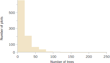
(b) Using the central limit theorem, what is the probability that the mean of the eight would be within 1 standard error of the mean?
(c) Why might you think that the probability that you calculated in (b) might not be very accurate?
7-19. Like hurricanes and earthquakes, geomagnetic storms are natural hazards with possible severe impact on the Earth. Severe storms can cause communication and utility breakdowns, leading to possible blackouts. The National Oceanic and Atmospheric Administration beams electron and proton flux data in various energy ranges to various stations on the Earth to help forecast possible disturbances. The following are 25 readings of proton flux in the 47-68 kEV range (units are in p/(cm2-sec-ster-MeV)) on the evening of December 28, 2011:
2310 2320 2010 10800 2190 3360 5640 2540 3360 11800 2010 3430 10600 7370 2160 3200 2020 2850 3500 10200 8550 9500 2260 7730 2250
(a) Find a point estimate of the mean proton flux in this time period.
(b) Find a point estimate of the standard deviation of the proton flux in this time period.
(c) Find an estimate of the standard error of the estimate in part (a).
(d) Find a point estimate for the median proton flux in this time period.
(e) Find a point estimate for the proportion of readings that are less than 5000 p/(cm2-sec-ster-MeV).
7-20. Wayne Collier designed an experiment to measure the fuel efficiency of his family car under different tire pressures. For each run, he set the tire pressure and then measured the miles he drove on a highway (I-95 between Mills River and Pisgah Forest, NC) until he ran out of fuel using 2 liters of fuel each time. To do this, he made some alterations to the normal flow of gasoline to the engine. In Wayne's words, “I inserted a T-junction into the fuel line just before the fuel filter, and a line into the passenger compartment of my car, where it joined with a graduated 2 liter Rubbermaid© bottle that I mounted in a box where the passenger seat is normally fastened. Then I sealed off the fuel-return line, which under normal operation sends excess fuel from the fuel pump back to the fuel tank.”
Suppose that you call the mean miles that he can drive with normal pressure in the tires μ. An unbiased estimate for μ is the mean of the sample runs, ![]() . But Wayne has a different idea. He decides to use the following estimator: He flips a fair coin. If the coin comes up heads, he will add five miles to each observation. If tails come up, he will subtract five miles from each observation.
. But Wayne has a different idea. He decides to use the following estimator: He flips a fair coin. If the coin comes up heads, he will add five miles to each observation. If tails come up, he will subtract five miles from each observation.
(a) Show that Wayne's estimate is, in fact, unbiased.
(b) Compare the standard deviation of Wayne's estimate with the standard deviation of the sample mean.
(c) Given your answer to (b), why does Wayne's estimate not make good sense scientifically?
7-21. Consider a Weibull distribution with shape parameter 1.5 and scale parameter 2.0. Generate a graph of the probability distribution. Does it look very much like a normal distribution? Construct a table similar to Table 7-1 by drawing 20 random samples of size n = 10 from this distribution. Compute the sample average from each sample and construct a normal probability plot of the sample averages. Do the sample averages seem to be normally distributed?
7-3 General Concepts of Point Estimation
7-3.1 UNBIASED ESTIMATORS
An estimator should be “close” in some sense to the true value of the unknown parameter. Formally, we say that ![]() is an unbiased estimator of θ if the expected value of
is an unbiased estimator of θ if the expected value of ![]() is equal to θ. This is equivalent to saying that the mean of the probability distribution of
is equal to θ. This is equivalent to saying that the mean of the probability distribution of ![]() (or the mean of the sampling distribution of
(or the mean of the sampling distribution of ![]() ) is equal to θ.
) is equal to θ.
Bias of an Estimator
The point estimator ![]() is an unbiased estimator for the parameter θ if
is an unbiased estimator for the parameter θ if
![]()
If the estimator is not unbiased, then the difference
![]()
is called the bias of the estimator ![]() .
.
When an estimator is unbiased, the bias is zero; that is, E(![]() ) − θ = 0.
) − θ = 0.
Example 7-4 Sample Mean and Variance are Unbiased Suppose that X is a random variable with mean μ and variance σ2. Let X1, X2,..., Xn be a random sample of size n from the population represented by X. Show that the sample mean ![]() and sample variance S2 are unbiased estimators of μ and σ2, respectively.
and sample variance S2 are unbiased estimators of μ and σ2, respectively.
First consider the sample mean. In Section 5.5 in Chapter 5, we showed that E(![]() ) = μ. Therefore, the sample mean
) = μ. Therefore, the sample mean ![]() is an unbiased estimator of the population mean μ.
is an unbiased estimator of the population mean μ.
Now consider the sample variance. We have
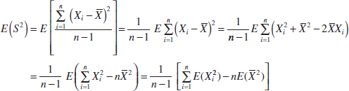
The last equality follows the equation for the mean of a linear function in Chapter 5. However, because E(![]() ) = μ2 + σ2 and E(
) = μ2 + σ2 and E(![]() 2) = μ2 + σ2/n, we have
2) = μ2 + σ2/n, we have
Therefore, the sample variance S2 is an unbiased estimator of the population variance σ2.
Although S2 is unbiased for σ2, S is a biased estimator of σ. For large samples, the bias is very small. However, there are good reasons for using S as an estimator of σ in samples from normal distributions as we will see in the next three chapters when we discuss confidence intervals and hypothesis testing.
Sometimes there are several unbiased estimators of the sample population parameter. For example, suppose that we take a random sample of size n = 10 from a normal population and obtain the data x1 = 12.8, x2 = 9.4, x3 = 8.7, x4 = 11.6, x5 = 13.1, x6 = 9.8, x7 = 14.1, x8 = 8.5, x9 = 12.1, x10 = 10.3. Now the sample mean is
![]()
the sample median is
![]()
and a 10% trimmed mean (obtained by discarding the smallest and largest 10% of the sample before averaging) is
![]()
We can show that all of these are unbiased estimates of μ. Because there is not a unique unbiased estimator, we cannot rely on the property of unbiasedness alone to select our estimator. We need a method to select among unbiased estimators. We suggest a method in the following section.
7-3.2 Variance of a Point Estimator
Suppose that ![]() 1 and
1 and ![]() 2 are unbiased estimators of θ. This indicates that the distribution of each estimator is centered at the true value of zero. However, the variance of these distributions may be different. Figure 7-7 illustrates the situation. Because
2 are unbiased estimators of θ. This indicates that the distribution of each estimator is centered at the true value of zero. However, the variance of these distributions may be different. Figure 7-7 illustrates the situation. Because ![]() 1 has a smaller variance than
1 has a smaller variance than ![]() 2, the estimator
2, the estimator ![]() 1 is more likely to produce an estimate close to the true value of θ. A logical principle of estimation when selecting among several unbiased estimators is to choose the estimator that has minimum variance.
1 is more likely to produce an estimate close to the true value of θ. A logical principle of estimation when selecting among several unbiased estimators is to choose the estimator that has minimum variance.
Minimum Variance Unbiased Estimator
If we consider all unbiased estimators of θ, the one with the smallest variance is called the minimum variance unbiased estimator (MVUE).
In a sense, the MVUE is most likely among all unbiased estimators to produce an estimate ![]() that is close to the true value of θ. It has been possible to develop methodology to identify the MVUE in many practical situations. Although this methodology is beyond the scope of this book, we give one very important result concerning the normal distribution.
that is close to the true value of θ. It has been possible to develop methodology to identify the MVUE in many practical situations. Although this methodology is beyond the scope of this book, we give one very important result concerning the normal distribution.
If X1, X2,..., Xn is a random sample of size n from a normal distribution with mean μ and variance σ2, the sample mean ![]() is the MVUE for μ.
is the MVUE for μ.
When we do not know whether an MVUE exists, we could still use a minimum variance principle to choose among competing estimators. Suppose, for example, we wish to estimate the mean of a population (not necessarily a normal population). We have a random sample of n observations X1, X2,..., Xn, and we wish to compare two possible estimators for μ: the sample mean ![]() and a single observation from the sample, say, Xi. Note that both
and a single observation from the sample, say, Xi. Note that both ![]() and Xi are unbiased estimators of μ; for the sample mean, we have V(
and Xi are unbiased estimators of μ; for the sample mean, we have V(![]() ) = σ2/n from Chapter 5 and the variance of any observation is V(Xi) = σ2. Because V(
) = σ2/n from Chapter 5 and the variance of any observation is V(Xi) = σ2. Because V(![]() ) < V(Xi) for sample sizes n ≥ 2, we would conclude that the sample mean is a better estimator of μ than a single observation Xi.
) < V(Xi) for sample sizes n ≥ 2, we would conclude that the sample mean is a better estimator of μ than a single observation Xi.
7-3.3 Standard Error: Reporting a Point Estimate
When the numerical value or point estimate of a parameter is reported, it is usually desirable to give some idea of the precision of estimation. The measure of precision usually employed is the standard error of the estimator that has been used.

FIGURE 7-7 The sampling distributions of two unbiased estimators ![]() 1 and
1 and ![]() 2.
2.
The standard error of an estimator ![]() is its standard deviation given by
is its standard deviation given by ![]() If the standard error involves unknown parameters that can be estimated, substitution of those values into
If the standard error involves unknown parameters that can be estimated, substitution of those values into ![]() produces an estimated standard error, denoted by
produces an estimated standard error, denoted by ![]() .
.
Sometimes the estimated standard error is denoted by ![]() or se(
or se(![]() ).
).
Suppose that we are sampling from a normal distribution with mean μ and variance σ2. Now the distribution of ![]() is normal with mean μ and variance σ2/n, so the standard error of
is normal with mean μ and variance σ2/n, so the standard error of ![]() is
is
![]()
If we did not know σ but substituted the sample standard deviation S into the preceding equation, the estimated standard error of ![]() would be
would be
![]()
When the estimator follows a normal distribution as in the preceding situation, we can be reasonably confident that the true value of the parameter lies within two standard errors of the estimate. Because many point estimators are normally distributed (or approximately so) for large n, this is a very useful result. Even when the point estimator is not normally distributed, we can state that so long as the estimator is unbiased, the estimate of the parameter will deviate from the true value by as much as four standard errors at most 6 percent of the time. Thus, a very conservative statement is that the true value of the parameter differs from the point estimate by at most four standard errors. See Chebyshev's inequality in the supplemental material on the Web site.
Example 7-5 Thermal Conductivity An article in the Journal of Heat Transfer (Trans. ASME, Sec. C, 96, 1974, p. 59) described a new method of measuring the thermal conductivity of Armco iron. Using a temperature of 100°F and a power input of 550 watts, the following 10 measurements of thermal conductivity (in Btu/hr-ft-°F) were obtained:
![]()
A point estimate of the mean thermal conductivity at 100°F and 550 watts is the sample mean or
![]()
The standard error of the sample mean is ![]() , and because σ is unknown, we may replace it by the sample standard deviation s = 0.284 to obtain the estimated standard error of
, and because σ is unknown, we may replace it by the sample standard deviation s = 0.284 to obtain the estimated standard error of ![]() as
as
![]()
Practical Interpretation: Notice that the standard error is about 0.2 percent of the sample mean, implying that we have obtained a relatively precise point estimate of thermal conductivity. If we can assume that thermal conductivity is normally distributed, 2 times the standard error is ![]() = 2(0.0898) = 0.1796, and we are highly confident that the true mean thermal conductivity is within the interval 41.924 ± 0.1796 or between 41.744 and 42.104.
= 2(0.0898) = 0.1796, and we are highly confident that the true mean thermal conductivity is within the interval 41.924 ± 0.1796 or between 41.744 and 42.104.
7.3.4 Bootstrap Standard Error
In some situations, the form of a point estimator is complicated, and standard statistical methods to find its standard error are difficult or impossible to apply. One example of these is S, the point estimator of the population standard deviation σ. Others occur with some of the standard probability distributions, such as the exponential and Weibull distributions. A relatively new computer-intensive technique, the bootstrap, can be used to solve this problem.
To explain how the bootstrap works, suppose that we have a random variable X with a known probability density function characterized by a parameter θ, say f(x; θ). Also assume that we have a random sample of data from this distribution, x1, x2,..., xn and that the estimate of θ based on this sample data is ![]() = 4.5. The bootstrap procedure would use the computer to generate bootstrap samples randomly from the probability distribution f(x; θ = 4.5) and calculate a bootstrap estimate
= 4.5. The bootstrap procedure would use the computer to generate bootstrap samples randomly from the probability distribution f(x; θ = 4.5) and calculate a bootstrap estimate ![]() B. This process is repeated nB times, resulting in:
B. This process is repeated nB times, resulting in:
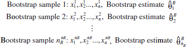
Typically, the number of bootstrap samples is nB = 100 or 200. The sample mean of the bootstrap estimates is
![]()
The bootstrap standard error of ![]() is just the sample standard deviation of the bootstrap estimates
is just the sample standard deviation of the bootstrap estimates ![]() or
or
![]()
Some authors use nB in the denominator of Equation 7-7.
Example 7-6 Bootstrap Standard Error A team of analytics specialists has been investigating the cycle time to process loan applications. The specialists' experience with the process informs them that cycle time is normally distributed with a mean of about 25 hours. A recent random sample of 10 applications gives the following (in hours):
![]()
The sample standard deviation of these observations is s = 3.11407. We want to find a bootstrap standard error for the sample standard deviation. We use a computer program to generate nB = 200 bootstrap samples from a normal distribution with a mean of 25 and a standard deviation of 3.11417. The first of these samples is:
![]()
from which we calculate s = 2.50635. After all 200 bootstrap samples were generated, the average of the bootstrap estimates of the standard deviation was 3.03972, and the bootstrap estimate of the standard error was 0.5464. The standard error is fairly large because the sample size here (n = 10) is fairly small.
In some problem situations, the distribution of the random variable is not known. The bootstrap can still be used in these situations. The procedure is to treat the data sample as a population and draw bootstrap samples from it. So, for example, if we had a sample of 25 observations, we would draw nB bootstrap samples by sampling with replacement from the original sample. Then we would proceed as in the preceding example to calculate the bootstrap estimate of the standard error for the statistic of interest.
7-3.5 Mean Squared Error of an Estimator
Sometimes it is necessary to use a biased estimator. In such cases, the mean squared error of the estimator can be important. The mean squared error of an estimator ![]() is the expected squared difference between
is the expected squared difference between ![]() and θ.
and θ.
Mean Squared Error of an Estimator
The mean squared error of an estimator ![]() of the parameter θ is defined as
of the parameter θ is defined as
![]()
The mean squared error can be rewritten as follows:
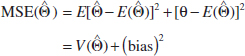
That is, the mean squared error of ![]() is equal to the variance of the estimator plus the squared bias. If
is equal to the variance of the estimator plus the squared bias. If ![]() is an unbiased estimator of θ, the mean squared error of
is an unbiased estimator of θ, the mean squared error of ![]() is equal to the variance of
is equal to the variance of ![]() .
.
The mean squared error is an important criterion for comparing two estimators. Let ![]() 1 and
1 and ![]() 2 be two estimators of the parameter θ, and let MSE (
2 be two estimators of the parameter θ, and let MSE (![]() 1) and MSE (
1) and MSE (![]() 2) be the mean squared errors of
2) be the mean squared errors of ![]() 1 and
1 and ![]() 2. Then the relative efficiency of
2. Then the relative efficiency of ![]() 2 to
2 to ![]() 1 is defined as
1 is defined as
![]()
If this relative efficiency is less than 1, we would conclude that ![]() 1 is a more efficient estimator of θ than
1 is a more efficient estimator of θ than ![]() 2 in the sense that it has a smaller mean squared error.
2 in the sense that it has a smaller mean squared error.
Sometimes we find that biased estimators are preferable to unbiased estimators because they have smaller mean squared error. That is, we may be able to reduce the variance of the estimator considerably by introducing a relatively small amount of bias. As long as the reduction in variance is larger than the squared bias, an improved estimator from a mean squared error viewpoint will result. For example, Fig. 7-8 is the probability distribution of a biased estimator ![]() 1 that has a smaller variance than the unbiased estimator
1 that has a smaller variance than the unbiased estimator ![]() 2. An estimate based on
2. An estimate based on ![]() 1 would more likely be close to the true value of θ than would an estimate based on
1 would more likely be close to the true value of θ than would an estimate based on ![]() 2. Linear regression analysis (Chapters 11 and 12) is an example of an application area in which biased estimators are occasionally used.
2. Linear regression analysis (Chapters 11 and 12) is an example of an application area in which biased estimators are occasionally used.
An estimator ![]() that has a mean squared error that is less than or equal to the mean squared error of any other estimator, for all values of the parameter θ, is called an optimal estimator of θ. Optimal estimators rarely exist.
that has a mean squared error that is less than or equal to the mean squared error of any other estimator, for all values of the parameter θ, is called an optimal estimator of θ. Optimal estimators rarely exist.
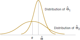
FIGURE 7-8 A biased estimator ![]() 1 that has smaller variance than the unbiased estimator
1 that has smaller variance than the unbiased estimator ![]() 2.
2.
![]() Problem available in WileyPLUS at instructor's discretion.
Problem available in WileyPLUS at instructor's discretion.
![]() Go Tutorial Tutoring problem available in WileyPLUS at instructor's discretion.
Go Tutorial Tutoring problem available in WileyPLUS at instructor's discretion.
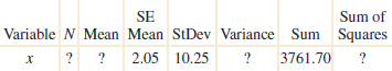
7-22. ![]() A computer software package calculated some numerical summaries of a sample of data. The results are displayed here:
A computer software package calculated some numerical summaries of a sample of data. The results are displayed here:
![]()
(a) Fill in the missing quantities.
(b) What is the estimate of the mean of the population from which this sample was drawn?
7-23. A computer software package calculated some numerical summaries of a sample of data. The results are displayed here:
(a) Fill in the missing quantities.
(b) What is the estimate of the mean of the population from which this sample was drawn?
7-24. ![]() Let X1 and X2 be independent random variables with mean μ and variance σ2. Suppose that we have two estimators of μ:
Let X1 and X2 be independent random variables with mean μ and variance σ2. Suppose that we have two estimators of μ:
![]()
(a) Are both estimators unbiased estimators of μ?
(b) What is the variance of each estimator?
7-25. Suppose that we have a random sample X1, X2,..., Xn from a population that is N(μ, σ2). We plan to use ![]() =
= ![]() to estimate σ2. Compute the bias in
to estimate σ2. Compute the bias in ![]() as an estimator of σ2 as a function of the constant c.
as an estimator of σ2 as a function of the constant c.
7-26. Suppose we have a random sample of size 2n from a population denoted by X, and E(X) = μ and V(X) = σ2. Let
![]()
be two estimators of μ. Which is the better estimator of μ? Explain your choice.
7-27. ![]() Let X1, X2,..., X7 denote a random sample from a population having mean μ and variance σ2. Consider the following estimators of μ:
Let X1, X2,..., X7 denote a random sample from a population having mean μ and variance σ2. Consider the following estimators of μ:

(a) Is either estimator unbiased?
(b) Which estimator is better? In what sense is it better? Calculate the relative efficiency of the two estimators.
7-28. ![]() Suppose that
Suppose that ![]() 1 and
1 and ![]() 2 are unbiased estimators of the parameter θ. We know that V(
2 are unbiased estimators of the parameter θ. We know that V(![]() 1) = 10 and V(
1) = 10 and V(![]() 2) = 4. Which estimator is better and in what sense is it better? Calculate the relative efficiency of the two estimators.
2) = 4. Which estimator is better and in what sense is it better? Calculate the relative efficiency of the two estimators.
7-29. Suppose that ![]() 1 and
1 and ![]() 2 are estimators of the parameter θ. We know that E(
2 are estimators of the parameter θ. We know that E(![]() 1) = θ, E(
1) = θ, E(![]() 2) = θ/2, V(
2) = θ/2, V(![]() 1) = 10, V(
1) = 10, V(![]() 2) = 4. Which estimator is better? In what sense is it better?
2) = 4. Which estimator is better? In what sense is it better?
7-30. Suppose that ![]() 1,
1, ![]() 2, and
2, and ![]() 3 are estimators of θ. We know that E(
3 are estimators of θ. We know that E(![]() 1) = E(
1) = E(![]() 2) = θ, E(
2) = θ, E(![]() 3) ≠ θ, V(
3) ≠ θ, V(![]() 1) = 12, V(
1) = 12, V(![]() 2) = 10 and E(
2) = 10 and E(![]() 3 − θ)2 = 6. Compare these three estimators. Which do you prefer? Why?
3 − θ)2 = 6. Compare these three estimators. Which do you prefer? Why?
7-31. Let three random samples of sizes n1 = 20, n2 = 10, and n3 = 8 be taken from a population with mean μ and variance σ2. Let ![]() , and
, and ![]() be the sample variances. Show that S2 =
be the sample variances. Show that S2 = ![]() /38 is an unbiased estimator of σ2.
/38 is an unbiased estimator of σ2.
7-32. ![]() (a) Show that
(a) Show that ![]() is a biased estimator of σ2.
is a biased estimator of σ2.
(b) Find the amount of bias in the estimator.
(c) What happens to the bias as the sample size n increases?
7-33. ![]() Let X1, X2,..., Xn be a random sample of size n from a population with mean μ and variance σ2.
Let X1, X2,..., Xn be a random sample of size n from a population with mean μ and variance σ2.
(a) Show that ![]() 2 is a biased estimator for μ2.
2 is a biased estimator for μ2.
(b) Find the amount of bias in this estimator.
(c) What happens to the bias as the sample size n increases?
7-34. ![]() Data on pull-off force (pounds) for connectors used in an automobile engine application are as follows: 79.3, 75.1, 78.2, 74.1, 73.9, 75.0, 77.6, 77.3, 73.8, 74.6, 75.5, 74.0, 74.7, 75.9, 72.9, 73.8, 74.2, 78.1, 75.4, 76.3, 75.3, 76.2, 74.9, 78.0, 75.1, 76.8.
Data on pull-off force (pounds) for connectors used in an automobile engine application are as follows: 79.3, 75.1, 78.2, 74.1, 73.9, 75.0, 77.6, 77.3, 73.8, 74.6, 75.5, 74.0, 74.7, 75.9, 72.9, 73.8, 74.2, 78.1, 75.4, 76.3, 75.3, 76.2, 74.9, 78.0, 75.1, 76.8.
(a) Calculate a point estimate of the mean pull-off force of all connectors in the population. State which estimator you used and why.
(b) Calculate a point estimate of the pull-off force value that separates the weakest 50% of the connectors in the population from the strongest 50%.
(c) Calculate point estimates of the population variance and the population standard deviation.
(d) Calculate the standard error of the point estimate found in part (a). Interpret the standard error.
(e) Calculate a point estimate of the proportion of all connectors in the population whose pull-off force is less than 73 pounds.
7-35. ![]() Data on the oxide thickness of semiconductor wafers are as follows: 425, 431, 416, 419, 421, 436, 418, 410, 431, 433, 423, 426, 410, 435, 436, 428, 411, 426, 409, 437, 422, 428, 413, 416.
Data on the oxide thickness of semiconductor wafers are as follows: 425, 431, 416, 419, 421, 436, 418, 410, 431, 433, 423, 426, 410, 435, 436, 428, 411, 426, 409, 437, 422, 428, 413, 416.
(a) Calculate a point estimate of the mean oxide thickness for all wafers in the population.
(b) Calculate a point estimate of the standard deviation of oxide thickness for all wafers in the population.
(c) Calculate the standard error of the point estimate from part (a).
(d) Calculate a point estimate of the median oxide thickness for all wafers in the population.
(e) Calculate a point estimate of the proportion of wafers in the population that have oxide thickness of more than 430 angstroms.
7-36. Suppose that X is the number of observed “successes” in a sample of n observations where p is the probability of success on each observation.
(a) Show that ![]() = X/n is an unbiased estimator of p.
= X/n is an unbiased estimator of p.
(b) Show that the standard error of ![]() is
is ![]() . How would you estimate the standard error?
. How would you estimate the standard error?
7-37. ![]() 1 and
1 and ![]() are the sample mean and sample variance from a population with mean μ1 and variance
are the sample mean and sample variance from a population with mean μ1 and variance ![]() . Similarly,
. Similarly, ![]() 2 and
2 and ![]() are the sample mean and sample variance from a second independent population with mean μ2 and variance
are the sample mean and sample variance from a second independent population with mean μ2 and variance ![]() . The sample sizes are n1 and n2, respectively.
. The sample sizes are n1 and n2, respectively.
(a) Show that ![]() 1 −
1 − ![]() 2 is an unbiased estimator of μ1 − μ2.
2 is an unbiased estimator of μ1 − μ2.
(b) Find the standard error of ![]() 1 −
1 − ![]() 2. How could you estimate the standard error?
2. How could you estimate the standard error?
(c) Suppose that both populations have the same variance; that is, ![]() . Show that
. Show that
![]()
is an unbiased estimator of σ2.
7-38. ![]() Two different plasma etchers in a semiconductor factory have the same mean etch rate μ. However, machine 1 is newer than machine 2 and consequently has smaller variability in etch rate. We know that the variance of etch rate for machine 1 is
Two different plasma etchers in a semiconductor factory have the same mean etch rate μ. However, machine 1 is newer than machine 2 and consequently has smaller variability in etch rate. We know that the variance of etch rate for machine 1 is ![]() , and for machine 2, it is
, and for machine 2, it is ![]() . Suppose that we have n1 independent observations on etch rate from machine 1 and n2 independent observations on etch rate from machine 2.
. Suppose that we have n1 independent observations on etch rate from machine 1 and n2 independent observations on etch rate from machine 2.
(a) Show that ![]() = α
= α ![]() 1 + (1 − α)
1 + (1 − α) ![]() 2 is an unbiased estimator of μ for any value of α between zero and one.
2 is an unbiased estimator of μ for any value of α between zero and one.
(b) Find the standard error of the point estimate of μ in part (a).
(c) What value of α would minimize the standard error of the point estimate of μ?
(d) Suppose that a = 4 and n1 = 2n2. What value of α would you select to minimize the standard error of the point estimate of μ? How “bad” would it be to arbitrarily choose α = 0.5 in this case?
7-39. Of n1 randomly selected engineering students at ASU, X1 owned an HP calculator, and of n2 randomly selected engineering students at Virginia Tech, X2 owned an HP calculator. Let p1 and p2 be the probability that randomly selected ASU and Virginia Tech engineering students, respectively, own HP calculators.
(a) Show that an unbiased estimate for p1 − p2 is (X1 / n1) = (X2 / n2).
(b) What is the standard error of the point estimate in part (a)?
(c) How would you compute an estimate of the standard error found in part (b)?
(d) Suppose that n1 = 200, X1 = 150, n2 = 250, and X2 = 185. Use the results of part (a) to compute an estimate of p1 − p2.
(e) Use the results in parts (b) through (d) to compute an estimate of the standard error of the estimate.
7-40. Suppose that the random variable X has a lognormal distribution with parameters θ = 1.5 and ω = 0.8. A sample of size n = 15 is drawn from this distribution. Find the standard error of the sample median of this distribution with the bootstrap method using nB = 200 bootstrap samples.
7-41. An exponential distribution is known to have a mean of 10. You want to find the standard error of the median of this distribution if a random sample of size 8 is drawn. Use the bootstrap method to find the standard error, using nB = 100 bootstrap samples.
7-42. Consider a normal random variable with mean 10 and standard deviation 4. Suppose that a random sample of size 16 is drawn from this distribution and the sample mean is computed. We know that the standard error of the sample mean in this case is ![]() . Use the bootstrap method with nB = 200 bootstrap samples to find the standard error of the sample mean. Compare the bootstrap standard error to the actual standard error.
. Use the bootstrap method with nB = 200 bootstrap samples to find the standard error of the sample mean. Compare the bootstrap standard error to the actual standard error.
7-43. Suppose that two independent random samples (of size n1 and n2) from two normal distributions are available. Explain how you would estimate the standard error of the difference in sample means ![]() 1 −
1 − ![]() 2 with the bootstrap method.
2 with the bootstrap method.
7-4 Methods of Point Estimation
The definitions of unbiasedness and other properties of estimators do not provide any guidance about how to obtain good estimators. In this section, we discuss methods for obtaining point estimators: the method of moments and the method of maximum likelihood. We also briefly discuss a Bayesian approach to parameter estimation. Maximum likelihood estimates are generally preferable to moment estimators because they have better efficiency properties. However, moment estimators are sometimes easier to compute. Both methods can produce unbiased point estimators.
7-4.1 Method of Moments
The general idea behind the method of moments is to equate population moments, which are defined in terms of expected values, to the corresponding sample moments. The population moments will be functions of the unknown parameters. Then these equations are solved to yield estimators of the unknown parameters.
Let X1, X2,..., Xn be a random sample from the probability distribution f(x) where f(x) can be a discrete probability mass function or a continuous probability density function. The kth population moment (or distribution moment) is E(Xk), k = 1, 2,.... The corresponding kth sample moment is ![]() = 1, 2,....
= 1, 2,....
To illustrate, the first population moment is E(X) = μ, and the first sample moment is ![]() . Thus, by equating the population and sample moments, we find that
. Thus, by equating the population and sample moments, we find that ![]() =
= ![]() . That is, the sample mean is the moment estimator of the population mean. In the general case, the population moments will be functions of the unknown parameters of the distribution, say, θ1, θ2,..., θm.
. That is, the sample mean is the moment estimator of the population mean. In the general case, the population moments will be functions of the unknown parameters of the distribution, say, θ1, θ2,..., θm.
Moment Estimators
Let X1, X2,..., Xn be a random sample from either a probability mass function or a probability density function with m unknown parameters θ1, θ2,..., θm. The moment estimators ![]() 1,
1, ![]() 2,...,
2,..., ![]() m are found by equating the first m population moments to the first m sample moments and solving the resulting equations for the unknown parameters.
m are found by equating the first m population moments to the first m sample moments and solving the resulting equations for the unknown parameters.
Example 7-7 Exponential Distribution Moment Estimator Suppose that X1, X2,..., Xn is a random sample from an exponential distribution with parameter λ. Now there is only one parameter to estimate, so we must equate E(X) to ![]() . For the exponential, E(X) = 1/λ. Therefore, E(X) =
. For the exponential, E(X) = 1/λ. Therefore, E(X) = ![]() results in 1/λ =
results in 1/λ = ![]() , so λ = 1 /
, so λ = 1 / ![]() , is the moment estimator of λ.
, is the moment estimator of λ.
As an example, suppose that the time to failure of an electronic module used in an automobile engine controller is tested at an elevated temperature to accelerate the failure mechanism. The time to failure is exponentially distributed. Eight units are randomly selected and tested, resulting in the following failure time (in hours): x1 = 11.96, x2 = 5.03, x3 = 67.40, x4 = 16.07, x5 = 31.50, x6 = 7.73, x7 = 11.10, and x8 = 22.38. Because ![]() = 21.65, the moment estimate of λ is
= 21.65, the moment estimate of λ is ![]() = 1/
= 1/![]() = 1/21.65 = 0.0462.
= 1/21.65 = 0.0462.
Example 7-8 Normal Distribution Moment Estimators Suppose that X1, X2,..., Xn is a random sample from a normal distribution with parameters μ and σ2. For the normal distribution, E(X) = μ and E(X2) = μ2 + σ2. Equating E(X) to X and E(X2) to ![]() gives
gives
![]()
Solving these equations gives the moment estimators
Practical Conclusion: Notice that the moment estimator of σ2 is not an unbiased estimator.
Example 7-9 Gamma Distribution Moment Estimators Suppose that X1, X2,..., Xn is a random sample from a gamma distribution with parameters r and λ. For the gamma distribution, E(X) = r/λ and E(X2) = r(r + 1)/λ2. The moment estimators are found by solving
![]()
The resulting estimators are
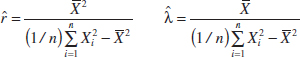
To illustrate, consider the time to failure data introduced following Example 7-7. For these data, ![]() = 21.65 and
= 21.65 and ![]() , so the moment estimates are
, so the moment estimates are
![]()
Interpretation: When r = 1, the gamma reduces to the exponential distribution. Because ![]() slightly exceeds unity, it is quite possible that either the gamma or the exponential distribution would provide a reasonable model for the data.
slightly exceeds unity, it is quite possible that either the gamma or the exponential distribution would provide a reasonable model for the data.
7-4.2 Method of Maximum Likelihood
One of the best methods of obtaining a point estimator of a parameter is the method of maximum likelihood. This technique was developed in the 1920s by a famous British statistician, Sir R. A. Fisher. As the name implies, the estimator will be the value of the parameter that maximizes the likelihood function.
Maximum Likelihood Estimator
Suppose that X is a random variable with probability distribution f(x;θ) where θ is a single unknown parameter. Let x1, x2,..., xn be the observed values in a random sample of size n. Then the likelihood function of the sample is
![]()
Note that the likelihood function is now a function of only the unknown parameter θ. The maximum likelihood estimator (MLE) of θ is the value of θ that maximizes the likelihood function L(θ).
In the case of a discrete random variable, the interpretation of the likelihood function is simple. The likelihood function of the sample L(θ) is just the probability
![]()
That is, L(θ) is just the probability of obtaining the sample values x1, x2,..., xn. Therefore, in the discrete case, the maximum likelihood estimator is an estimator that maximizes the probability of occurrence of the sample values. Maximum likelihood estimators are generally preferable to moment estimators because they possess good efficiency properties.
Example 7-10 Bernoulli Distribution MLE Let X be a Bernoulli random variable. The probability mass function is
![]()
where p is the parameter to be estimated. The likelihood function of a random sample of size n is
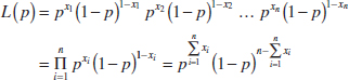
We observe that if ![]() maximizes L(p),
maximizes L(p), ![]() also maximizes ln L(p). Therefore,
also maximizes ln L(p). Therefore,
![]()
Now,
Equating this to zero and solving for p yields ![]() = (1/n)
= (1/n)![]() . Therefore, the maximum likelihood estimator of p is
. Therefore, the maximum likelihood estimator of p is
![]()
Suppose that this estimator were applied to the following situation: n items are selected at random from a production line, and each item is judged as either defective (in which case we set xi = 1) or nondefective (in which case we set xi = 0). Then ![]() is the number of defective units in the sample, and
is the number of defective units in the sample, and ![]() is the sample proportion defective. The parameter p is the population proportion defective, and it seems intuitively quite reasonable to use
is the sample proportion defective. The parameter p is the population proportion defective, and it seems intuitively quite reasonable to use ![]() as an estimate of p.
as an estimate of p.
Although the interpretation of the likelihood function just given is confined to the discrete random variable case, the method of maximum likelihood can easily be extended to a continuous distribution. We now give two examples of maximum likelihood estimation for continuous distributions.
Example 7-11 Normal Distribution MLE Let X be normally distributed with unknown μ and known variance σ2. The likelihood function of a random sample of size n, say X1, X2,..., Xn, is

Now
![]()
![]()
Equating this last result to zero and solving for μ yields

Conclusion: The sample mean is the maximum likelihood estimator of μ. Notice that this is identical to the moment estimator.
Example 7-12 Exponential Distribution MLE Let X be exponentially distributed with parameter λ. The likelihood function of a random sample of size n, say, X1, X2,..., Xn, is
![]()
The log likelihood is
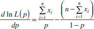
![]()
Now
![]()
and upon equating this last result to zero, we obtain
![]()
Conclusion: Thus, the maximum likelihood estimator of λ is the reciprocal of the sample mean. Notice that this is the same as the moment estimator.
It is easy to illustrate graphically just how the method of maximum likelihood works. Figure 7-9(a) plots the log of the likelihood function for the exponential parameter from Example 7-12, using the n = 8 observations on failure time given following Example 7-6. It is common for the log likelihood function to be negative. We found that the estimate of λ was ![]() = 0.0462. From Example 7-12, we know that this is a maximum likelihood estimate. Figure 7-9(a) shows clearly that the log likelihood function is maximized at a value of λ that is approximately equal to 0.0462. Notice that the log likelihood function is relatively flat in the region of the maximum. This implies that the parameter is not estimated very precisely. If the parameter were estimated precisely, the log likelihood function would be very peaked at the maximum value. The sample size here is relatively small, and this has led to the imprecision in estimation. This is illustrated in Fig. 7-9(b) where we have plotted the difference in log likelihoods for the maximum value, assuming that the sample sizes were n = 8, 20, and 40 but that the sample average time to failure remained constant at
= 0.0462. From Example 7-12, we know that this is a maximum likelihood estimate. Figure 7-9(a) shows clearly that the log likelihood function is maximized at a value of λ that is approximately equal to 0.0462. Notice that the log likelihood function is relatively flat in the region of the maximum. This implies that the parameter is not estimated very precisely. If the parameter were estimated precisely, the log likelihood function would be very peaked at the maximum value. The sample size here is relatively small, and this has led to the imprecision in estimation. This is illustrated in Fig. 7-9(b) where we have plotted the difference in log likelihoods for the maximum value, assuming that the sample sizes were n = 8, 20, and 40 but that the sample average time to failure remained constant at ![]() = 21.65. Notice how much steeper the log likelihood is for n = 20 in comparison to n = 8, and for n = 40 in comparison to both smaller sample sizes.
= 21.65. Notice how much steeper the log likelihood is for n = 20 in comparison to n = 8, and for n = 40 in comparison to both smaller sample sizes.

FIGURE 7-9 Log likelihood for the exponential distribution, using the failure time data. (a) Log likelihood with n = 8 (original data). (b) Log likelihood if n = 8, 20, and 40.
The method of maximum likelihood can be used in situations that have several unknown parameters, say, θ1, θ2,..., θk to estimate. In such cases, the likelihood function is a function of the k unknown parameters θ1, θ2,..., θk, and the maximum likelihood estimators {![]() i} would be found by equating the k partial derivatives ∂L(θ1, θ2,..., θk)/∂θi, i = 1, 2,..., k to zero and solving the resulting system of equations.
i} would be found by equating the k partial derivatives ∂L(θ1, θ2,..., θk)/∂θi, i = 1, 2,..., k to zero and solving the resulting system of equations.
Example 7-13 Normal Distribution MLEs For μ and σ2 Let X be normally distributed with mean μ and variance σ2 where both μ and σ2 are unknown. The likelihood function for a random sample of size n is

and
![]()
Now
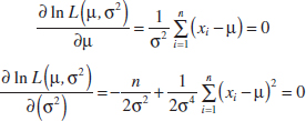
The solutions to these equations yield the maximum likelihood estimators
![]()
Conclusion: Once again, the maximum likelihood estimators are equal to the moment estimators.
Properties of the Maximum Likelihood Estimator
As noted previously, the method of maximum likelihood is often the estimation method that we prefer because it produces estimators with good statistical properties. We summarize these properties as follows.
Properties of a Maximum Likelihood Estimator
Under very general and not restrictive conditions when the sample size n is large and if ![]() is the maximum likelihood estimator of the parameter θ,
is the maximum likelihood estimator of the parameter θ,
 is an approximately unbiased estimator for θ[E()]
  θ,
θ,- The variance of is nearly as small as the variance that could be obtained with any other estimator.
- has an approximate normal distribution.
Properties 1 and 2 essentially state that the maximum likelihood estimator is approximately an MVUE. This is a very desirable result and, coupled with the facts that it is fairly easy to obtain in many situations and has an asymptotic normal distribution (the “asymptotic” means “when n is large”), explains why the maximum likelihood estimation technique is widely used. To use maximum likelihood estimation, remember that the distribution of the population must be either known or assumed.
To illustrate the “large-sample” or asymptotic nature of these properties, consider the maximum likelihood estimator for σ2, the variance of the normal distribution, in Example 7-13. It is easy to show that
![]()
The bias is
![]()
Because the bias is negative, ![]() 2 tends to underestimate the true variance σ2. Note that the bias approaches zero as n increases. Therefore,
2 tends to underestimate the true variance σ2. Note that the bias approaches zero as n increases. Therefore, ![]() 2 is an asymptotically unbiased estimator for σ2.
2 is an asymptotically unbiased estimator for σ2.
We now give another very important and useful property of maximum likelihood estimators.
Invariance Property
Let ![]() 1,
1, ![]() 2,...,
2,..., ![]() k be the maximum likelihood estimators of the parameters θ1, θ2,..., θk. Then the maximum likelihood estimator of any function h(θ1, θ2,..., θk) of these parameters is the same function h(
k be the maximum likelihood estimators of the parameters θ1, θ2,..., θk. Then the maximum likelihood estimator of any function h(θ1, θ2,..., θk) of these parameters is the same function h(![]() 1,
1, ![]() 2, ...,
2, ..., ![]() k) of the estimators
k) of the estimators ![]() 1,
1, ![]() 2,...,
2,..., ![]() k.
k.
Example 7-14 In the normal distribution case, the maximum likelihood estimators of μ and σ2 were ![]() =
= ![]() and
and ![]() 2 =
2 = ![]() , respectively. To obtain the maximum likelihood estimator of the function h(μ, σ2) =
, respectively. To obtain the maximum likelihood estimator of the function h(μ, σ2) = ![]() = σ, substitute the estimators
= σ, substitute the estimators ![]() and
and ![]() 2 into the function h, which yields
2 into the function h, which yields
![]()
Conclusion: The maximum likelihood estimator of the standard deviation σ is not the sample standard deviation S.
Complications in Using Maximum Likelihood Estimation
Although the method of maximum likelihood is an excellent technique, sometimes complications arise in its use. For example, it is not always easy to maximize the likelihood function because the equation(s) obtained from dL(θ)/dθ = 0 may be difficult to solve. Furthermore, it may not always be possible to use calculus methods directly to determine the maximum of L(θ). These points are illustrated in the following two examples.
Example 7-15 Uniform Distribution MLE Let X be uniformly distributed on the interval 0 to a. Because the density function is f(x) = 1/a for 0 ≤ x ≤ a and zero otherwise, the likelihood function of a random sample of size n is
![]()
for
![]()
Note that the slope of this function is not zero anywhere. That is, as long as max(xi) ≤ a, the likelihood is 1/an, which is positive, but when a < max(xi), the likelihood goes to zero as illustrated in Fig. 7-10. Therefore, calculus methods cannot be used directly because the maximum value of the likelihood function occurs at a point of discontinuity. However, because d/da(a−n) = −n/an+1 is less than zero for all values of a > 0, a−n is a decreasing function of a. This implies that the maximum of the likelihood function L(a) occurs at the lower boundary point. The figure clearly shows that we could maximize L(a) by setting â equal to the smallest value that it could logically take on, which is max(xi). Clearly, a cannot be smaller than the largest sample observation, so setting â equal to the largest sample value is reasonable.

FIGURE 7-10 The likelihood function for the uniform distribution in Example 7-15.
Example 7-16 Gamma Distribution MLE Let X1, X2,..., Xn be a random sample from the gamma distribution. The log of the likelihood function is

The derivatives of the log likelihood are
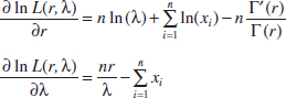
When the derivatives are equated to zero, we obtain the equations that must be solved to find the maximum likelihood estimators of r and λ:
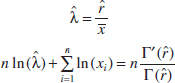
There is no closed form solution to these equations.
Figure 7-11 is a graph of the log likelihood for the gamma distribution using the n = 8 observations on failure time introduced previously. Figure 7-11a is the log likelihood surface as a function of r and λ, and Figure 7-11b is a contour plot. These plots reveal that the log likelihood is maximized at approximately ![]() = 1.75 and
= 1.75 and ![]() = 0.08. Many statistics computer programs use numerical techniques to solve for the maximum likelihood estimates when no simple solution exists.
= 0.08. Many statistics computer programs use numerical techniques to solve for the maximum likelihood estimates when no simple solution exists.
7-4.3 Bayesian Estimation of Parameters
This book uses methods of statistical inference based on the information in the sample data. In effect, these methods interpret probabilities as relative frequencies. Sometimes we call probabilities that are interpreted in this manner objective probabilities. Another approach to statistical inference, called the Bayesian approach, combines sample information with other information that may be available prior to collecting the sample. In this section, we briefly illustrate how this approach may be used in parameter estimation.
Suppose that the random variable X has a probability distribution that is a function of one parameter θ. We will write this probability distribution as f(x | θ). This notation implies that the exact form of the distribution of X is conditional on the value assigned to θ. The classical approach to estimation would consist of taking a random sample of size n from this distribution and then substituting the sample values xi into the estimator for θ. This estimator could have been developed using the maximum likelihood approach, for example.

FIGURE 7-11 Log likelihood for the gamma distribution using the failure time data. (a) Log likelihood surface. (b) Contour plot.
Suppose that we have some additional information about θ and that we can summarize that information in the form of a probability distribution for θ, say, f(θ). This probability distribution is often called the prior distribution for θ, and suppose that the mean of the prior is μ0 and the variance is ![]() . This is a very novel concept insofar as the rest of this book is concerned because we are now viewing the parameter θ as a random variable. The probabilities associated with the prior distribution are often called subjective probabilities because they usually reflect the analyst's degree of belief regarding the true value of θ. The Bayesian approach to estimation uses the prior distribution for θ, f(θ), and the joint probability distribution of the sample, say, f(x1, x2,..., xn|θ), to find a posterior distribution for θ, say, f(θ|x1, x2,..., xn). This posterior distribution contains information from both the sample and the prior distribution for θ. In a sense, it expresses our degree of belief regarding the true value of θ after observing the sample data. It is easy conceptually to find the posterior distribution. The joint probability distribution of the sample X1, X2,..., Xn and the parameter θ (remember that θ is a random variable) is
. This is a very novel concept insofar as the rest of this book is concerned because we are now viewing the parameter θ as a random variable. The probabilities associated with the prior distribution are often called subjective probabilities because they usually reflect the analyst's degree of belief regarding the true value of θ. The Bayesian approach to estimation uses the prior distribution for θ, f(θ), and the joint probability distribution of the sample, say, f(x1, x2,..., xn|θ), to find a posterior distribution for θ, say, f(θ|x1, x2,..., xn). This posterior distribution contains information from both the sample and the prior distribution for θ. In a sense, it expresses our degree of belief regarding the true value of θ after observing the sample data. It is easy conceptually to find the posterior distribution. The joint probability distribution of the sample X1, X2,..., Xn and the parameter θ (remember that θ is a random variable) is
![]()
and the marginal distribution of X1, X2,..., Xn is
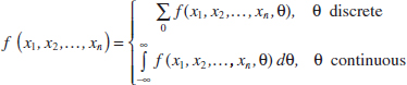
Therefore, the desired distribution is
![]()
We define the Bayes estimator of θ as the value ![]() that corresponds to the mean of the posterior distribution f(θ|x1, x2,..., xn).
that corresponds to the mean of the posterior distribution f(θ|x1, x2,..., xn).
Sometimes the mean of the posterior distribution of θ can be determined easily. As a function of θ, f(θ|x1,..., xn) is a probability density function and x1,..., xn are just constants. Because θ enters into f(θ|x1,..., xn) only through f(x1,..., xn, θ) if f(x1,..., xn, θ) because a function of θ is recognized as a well-known probability function, the posterior mean of θ can be deduced from the well-known distribution without integration or even calculation of f(x1,..., xn).
Example 7-17 Bayes Estimator for the Mean of a Normal Distribution Let X1, X2,..., Xn be a random sample from the normal distribution with mean μ and variance σ2 where μ is unknown and σ2 is known. Assume that the prior distribution for μ is normal with mean μ0 and variance ![]() ; that is,
; that is,
![]()
The joint probability distribution of the sample is

Thus, the joint probability distribution of the sample and μ is
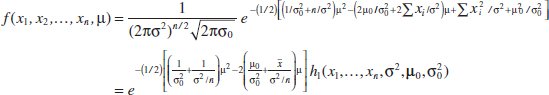
Upon completing the square in the exponent,

where hi(x1,..., xn, σ2, μ0, ![]() ) is a function of the observed values and the parameters σ2, μ0, and
) is a function of the observed values and the parameters σ2, μ0, and ![]() .
.
Now, because f(x1,..., xn) does not depend on μ,

This is recognized as a normal probability density function with posterior mean
![]()
and posterior variance
![]()
Consequently, the Bayes estimate of μ is a weighted average of μ0 and ![]() . For purposes of comparison, note that the maximum likelihood estimate of μ is
. For purposes of comparison, note that the maximum likelihood estimate of μ is ![]() =
= ![]() .
.
To illustrate, suppose that we have a sample of size n = 10 from a normal distribution with unknown mean μ and variance σ2 = 4. Assume that the prior distribution for μ is normal with mean μ0 = 0 and variance ![]() = 1. If the sample mean is 0.75, the Bayes estimate of μ is
= 1. If the sample mean is 0.75, the Bayes estimate of μ is
![]()
Conclusion: Note that the maximum likelihood estimate of μ is ![]() = 0.75. The Bayes estimate is between the maximum likelihood estimate and the prior mean.
= 0.75. The Bayes estimate is between the maximum likelihood estimate and the prior mean.
A relationship exists between the Bayes estimator for a parameter and the maximum likelihood estimator of the same parameter. For large sample sizes, the two are nearly equivalent. In general, the difference are the two estimators is small compared to 1/![]() . In practical problems, a moderate sample size will produce approximately the same estimate by either the Bayes or maximum likelihood method if the sample results are consistent with the assumed prior information. If the sample results are inconsistent with the prior assumptions, the Bayes estimate may differ considerably from the maximum likelihood estimate. In these circumstances, if the sample results are accepted as being correct, the prior information must be incorrect. The maximum likelihood estimate would then be the better estimate to use.
. In practical problems, a moderate sample size will produce approximately the same estimate by either the Bayes or maximum likelihood method if the sample results are consistent with the assumed prior information. If the sample results are inconsistent with the prior assumptions, the Bayes estimate may differ considerably from the maximum likelihood estimate. In these circumstances, if the sample results are accepted as being correct, the prior information must be incorrect. The maximum likelihood estimate would then be the better estimate to use.
If the sample results are very different from the prior information, the Bayes estimator will always tend to produce an estimate that is between the maximum likelihood estimate and the prior assumptions. This was illustrated in Example 7-16. If there is more inconsistency between the prior information and the sample, there will be more difference between the two estimates.
Exercises FOR SECTION 7-4
![]() Problem available in WileyPLUS at instructor's discretion.
Problem available in WileyPLUS at instructor's discretion.
![]() Go Tutorial Tutoring problem available in WileyPLUS at instructor's discretion.
Go Tutorial Tutoring problem available in WileyPLUS at instructor's discretion.
7-44. ![]() Let X be a geometric random variable with parameter p. Find the maximum likelihood estimator of p based on a random sample of size n.
Let X be a geometric random variable with parameter p. Find the maximum likelihood estimator of p based on a random sample of size n.
7-45. ![]() Consider the Poisson distribution with parameter λ. Find the maximum likelihood estimator of λ, based on a random sample of size n.
Consider the Poisson distribution with parameter λ. Find the maximum likelihood estimator of λ, based on a random sample of size n.
7-46. Let X be a random variable with the following probability distribution:
![]()
Find the maximum likelihood estimator of θ based on a random sample of size n.
7-47. Consider the shifted exponential distribution
![]()
When θ = 0, this density reduces to the usual exponential distribution. When θ > 0, there is positive probability only to the right of θ.
(a) Find the maximum likelihood estimator of λ and θ based on a random sample of size n.
(b) Describe a practical situation in which one would suspect that the shifted exponential distribution is a plausible model.
7-48. ![]() Consider the probability density function
Consider the probability density function
![]()
Find the maximum likelihood estimator for θ.
7-49. Let X1, X2,..., Xn be uniformly distributed on the interval 0 to a. Show that the moment estimator of a is â = 2![]() . Is this an unbiased estimator? Discuss the reasonableness of this estimator.
. Is this an unbiased estimator? Discuss the reasonableness of this estimator.
7-50. Consider the probability density function
![]()
(a) Find the value of the constant c.
(b) What is the moment estimator for θ?
(c) Show that ![]() = 3
= 3![]() is an unbiased estimator for θ.
is an unbiased estimator for θ.
(d) Find the maximum likelihood estimator for θ.
7-51. The Rayleigh distribution has probability density function
![]()
(a) It can be shown that E(X2) = 2θ. Use this information to construct an unbiased estimator for θ.
(b) Find the maximum likelihood estimator of θ. Compare your answer to part (a).
(c) Use the invariance property of the maximum likelihood estimator to find the maximum likelihood estimator of the median of the Raleigh distribution.
7-52. Let X1, X2,..., Xn be uniformly distributed on the interval 0 to a. Recall that the maximum likelihood estimator of a is â = max(Xi).
(a) Argue intuitively why â cannot be an unbiased estimator for a.
(b) Suppose that E(â) = na/(n + 1). Is it reasonable that â consistently underestimates a? Show that the bias in the estimator approaches zero as n gets large.
(c) Propose an unbiased estimator for a.
(d) Let Y = max(Xi). Use the fact that Y ≤ y if and only if each Xi ≤ y to derive the cumulative distribution function of Y. Then show that the probability density function of Y is
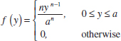
Use this result to show that the maximum likelihood estimator for a is biased.
(e) We have two unbiased estimators for a: the moment estimator â1 = 2![]() and â2 = [(n + 1)/n] max(Xi), where max(Xi) is the largest observation in a random sample of size n. It can be shown that V(â1) = a2/(3n) and that V(â2) = a2/[n(n + 2)]. Show that if n > 1, â2 is a better estimator than â. In what sense is it a better estimator of a?
and â2 = [(n + 1)/n] max(Xi), where max(Xi) is the largest observation in a random sample of size n. It can be shown that V(â1) = a2/(3n) and that V(â2) = a2/[n(n + 2)]. Show that if n > 1, â2 is a better estimator than â. In what sense is it a better estimator of a?
7-53. Consider the Weibull distribution
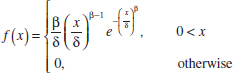
(a) Find the likelihood function based on a random sample of size n. Find the log likelihood.
(b) Show that the log likelihood is maximized by solving the following equations
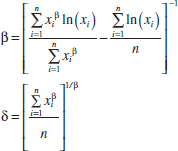
(c) What complications are involved in solving the two equations in part (b)?
7-54. Reconsider the oxide thickness data in Exercise 7-35 and suppose that it is reasonable to assume that oxide thickness is normally distributed.
(a) Compute the maximum likelihood estimates of μ and σ2.
(b) Graph the likelihood function in the vicinity of ![]() and
and ![]() 2, the maximum likelihood estimates, and comment on its shape.
2, the maximum likelihood estimates, and comment on its shape.
(c) Suppose that the sample size was larger (n = 40) but the maximum likelihood estimates were numerically equal to the values obtained in part (a). Graph the likelihood function for n = 40, compare it to the one from part (b), and comment on the effect of the larger sample size.
7-55. Suppose that X is a normal random variable with unknown mean μ and known variance σ2. The prior distribution for μ is a normal distribution with mean μ0 and variance ![]() . Show that the Bayes estimator for μ becomes the maximum likelihood estimator when the sample size n is large.
. Show that the Bayes estimator for μ becomes the maximum likelihood estimator when the sample size n is large.
7-56. Suppose that X is a normal random variable with unknown mean μ and known variance σ2. The prior distribution for μ is a uniform distribution defined over the interval [a, b].
(a) Find the posterior distribution for μ.
(b) Find the Bayes estimator for μ.
7-57. Suppose that X is a Poisson random variable with parameter λ. Let the prior distribution for λ be a gamma distribution with parameters m + 1 and (m + 1)/λ0.
(a) Find the posterior distribution for λ.
(b) Find the Bayes estimator for λ.
7-58. ![]() Suppose that X is a normal random variable with unknown mean and known variance σ2 = 9. The prior distribution for μ is normal with μ0 = 4 and
Suppose that X is a normal random variable with unknown mean and known variance σ2 = 9. The prior distribution for μ is normal with μ0 = 4 and ![]() = 1. A random sample of n = 25 observations is taken, and the sample mean is
= 1. A random sample of n = 25 observations is taken, and the sample mean is ![]() = 4.85.
= 4.85.
(a) Find the Bayes estimate of μ.
(b) Compare the Bayes estimate with the maximum likelihood estimate.
7-59. ![]() The weight of boxes of candy is a normal random variable with mean μ and variance 1/10 pound. The prior distribution for μ is normal with mean 5.03 pound and variance 1/25 pound. A random sample of 10 boxes gives a sample mean of
The weight of boxes of candy is a normal random variable with mean μ and variance 1/10 pound. The prior distribution for μ is normal with mean 5.03 pound and variance 1/25 pound. A random sample of 10 boxes gives a sample mean of ![]() = 5.05 pounds.
= 5.05 pounds.
(a) Find the Bayes estimate of μ.
(b) Compare the Bayes estimate with the maximum likelihood estimate.
7-60. ![]() The time between failures of a machine has an exponential distribution with parameter λ. Suppose that the prior distribution for λ is exponential with mean 100 hours. Two machines are observed, and the average time between failures is
The time between failures of a machine has an exponential distribution with parameter λ. Suppose that the prior distribution for λ is exponential with mean 100 hours. Two machines are observed, and the average time between failures is ![]() = 1125 hours.
= 1125 hours.
(a) Find the Bayes estimate for λ.
(b) What proportion of the machines do you think will fail before 1000 hours?
Supplemental Exercises
![]() Problem available in WileyPLUS at instructor's discretion.
Problem available in WileyPLUS at instructor's discretion.
![]() Go Tutorial Tutoring problem available in WileyPLUS at instructor's discretion.
Go Tutorial Tutoring problem available in WileyPLUS at instructor's discretion.
7-61. ![]() Transistors have a life that is exponentially distributed with parameter λ. A random sample of n transistors is taken. What is the joint probability density function of the sample?
Transistors have a life that is exponentially distributed with parameter λ. A random sample of n transistors is taken. What is the joint probability density function of the sample?
7-62. Suppose that a random variable is normally distributed with mean μ and variance σ2, and we draw a random sample of five observations from this distribution. What is the joint probability density function of the sample?
7-63. ![]() Suppose that X is uniformly distributed on the interval from 0 to 1. Consider a random sample of size 4 from X. What is the joint probability density function of the sample?
Suppose that X is uniformly distributed on the interval from 0 to 1. Consider a random sample of size 4 from X. What is the joint probability density function of the sample?
7-64. ![]() A procurement specialist has purchased 25 resistors from vendor 1 and 30 resistors from vendor 2. Let X1,1, X1,2,..., X1,25 represent the vendor 1 observed resistances, which are assumed to be normally and independently distributed with mean 100 ohms and standard deviation 1.5 ohms. Similarly, let X2,1, X2,2,..., X2,30 represent the vendor 2 observed resistances, which are assumed to be normally and independently distributed with mean 105 ohms and standard deviation of 2.0 ohms. What is the sampling distribution of
A procurement specialist has purchased 25 resistors from vendor 1 and 30 resistors from vendor 2. Let X1,1, X1,2,..., X1,25 represent the vendor 1 observed resistances, which are assumed to be normally and independently distributed with mean 100 ohms and standard deviation 1.5 ohms. Similarly, let X2,1, X2,2,..., X2,30 represent the vendor 2 observed resistances, which are assumed to be normally and independently distributed with mean 105 ohms and standard deviation of 2.0 ohms. What is the sampling distribution of ![]() 1 −
1 − ![]() 2? What is the standard error of
2? What is the standard error of ![]() 1 −
1 − ![]() 2?
2?
7-65. ![]() A random sample of 36 observations has been drawn from a normal distribution with mean 50 and standard deviation 12. Find the probability that the sample mean is in the interval 47 ≤ X ≤ 53. Is the assumption of normality important? Why?
A random sample of 36 observations has been drawn from a normal distribution with mean 50 and standard deviation 12. Find the probability that the sample mean is in the interval 47 ≤ X ≤ 53. Is the assumption of normality important? Why?
7-66. ![]() A random sample of n = 9 structural elements is tested for compressive strength. We know that the true mean compressive strength μ = 5500 psi and the standard deviation is σ = 100 psi. Find the probability that the sample mean compressive strength exceeds 4985 psi.
A random sample of n = 9 structural elements is tested for compressive strength. We know that the true mean compressive strength μ = 5500 psi and the standard deviation is σ = 100 psi. Find the probability that the sample mean compressive strength exceeds 4985 psi.
7-67. A normal population has a known mean 50 and known variance σ2 = 2. A random sample of n = 16 is selected from this population, and the sample mean is ![]() = 52. How unusual is this result?
= 52. How unusual is this result?
7-68. ![]() A random sample of size n = 16 is taken from a normal population with μ = 40 and σ2 = 5. Find the probability that the sample mean is less than or equal to 37.
A random sample of size n = 16 is taken from a normal population with μ = 40 and σ2 = 5. Find the probability that the sample mean is less than or equal to 37.
7-69. A manufacturer of semiconductor devices takes a random sample of 100 chips and tests them, classifying each chip as defective or nondefective. Let Xi = 0 if the chip is nondefective and Xi = 1 if the chip is defective. The sample fraction defective is
![]()
What is the sampling distribution of the random variable ![]() ?
?
7-70. ![]() Go Tutorial Let X be a random variable with mean μ and variance σ2. Given two independent random samples of sizes n1 and n2, with sample means
Go Tutorial Let X be a random variable with mean μ and variance σ2. Given two independent random samples of sizes n1 and n2, with sample means ![]() 1 and
1 and ![]() 2, show that
2, show that
![]()
is an unbiased estimator for μ. If ![]() 1 and
1 and ![]() 2 are independent, find the value of a that minimizes the standard error of
2 are independent, find the value of a that minimizes the standard error of ![]() .
.
7-71. ![]() A random variable x has probability density function
A random variable x has probability density function
![]()
Find the maximum likelihood estimator for θ.
7-72. Let f(x) = θxθ−1, 0 < θ < ∞ and 0 < x < 1. Show that ![]() = −n/
= −n/![]() is the maximum likelihood estimator for θ.
is the maximum likelihood estimator for θ.
7-73. Let f(x) = (1/θ)x(1−θ)/θ, 0 < x < 1, and 0 < θ < ∞. Show that ![]() = −(1/n)
= −(1/n)![]() ln(Xi) is the maximum likelihood estimator for θ and that
ln(Xi) is the maximum likelihood estimator for θ and that ![]() is an unbiased estimator for q.
is an unbiased estimator for q.
7-74. You plan to use a rod to lay out a square, each side of which is the length of the rod. The length of the rod is μ, which is unknown. You are interested in estimating the area of the square, which is μ2. Because μ is unknown, you measure it n times, obtaining observations X1, X2,..., Xn. Suppose that each measurement is unbiased for μ with variance σ2.
(a) Show that ![]() 2 is a biased estimate of the area of the square.
2 is a biased estimate of the area of the square.
(b) Suggest an estimator that is unbiased.
7-75. An electric utility has placed special meters on 10 houses in a subdivision that measures the energy consumed (demand) at each hour of the day. The company is interested in the energy demand at one specific hour—the hour at which the system experiences the peak consumption. The data from these 10 meters are as follows (in KW): 23.1, 15.6, 17.4, 20.1, 19.8, 26.4, 25.1, 20.5, 21.9, and 28.7. If μ is the true mean peak demand for the 10 houses in this group of houses having the special meters, estimate μ. Now suppose that the utility wants to estimate the demand at the peak hour for all 5000 houses in this subdivision. Let θ be this quantity. Estimate θ using the data given. Estimate the proportion of houses in the subdivision that demand at least 20 KW at the hour of system peak.
Mind-Expanding Exercises
7-76. A lot consists of N transistors, and of these, M(M ≤ N) are defective. We randomly select two transistors without replacement from this lot and determine whether they are defective or nondefective. The random variable
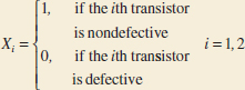
Determine the joint probability function for X1 and X2. What are the marginal probability functions for X1 and X2? Are X1 and X2 independent random variables?
7-77. When the sample standard deviation is based on a random sample of size n from a normal population, it can be shown that S is a biased estimator for σ. Specifically,
![]()
(a) Use this result to obtain an unbiased estimator for σ of the form cnS, when the constant cn depends on the sample size n.
(b) Find the value of cn for n = 10 and n = 25. Generally, how well does S perform as an estimator of σ for large n with respect to bias?
7-78. An operator using a gauge measure collection of n randomly selected parts twice. Let Xi and Yi denote the measured values for the ith part. Assume that these two random variables are independent and normally distributed and that both have true mean μi and variance σ2.
(a) Show that the maximum likelihood estimator of σ2 is ![]() .
.
(b) Show that ![]() 2 is a biased estimator for
2 is a biased estimator for ![]() 2. What happens to the bias as n becomes large?
2. What happens to the bias as n becomes large?
(c) Find an unbiased estimator for σ2.
7-79. Consistent Estimator. Another way to measure the closeness of an estimator ![]() to the parameter θ is in terms of consistency. If
to the parameter θ is in terms of consistency. If ![]() n is an estimator of θ based on a random sample of n observations,
n is an estimator of θ based on a random sample of n observations, ![]() n is consistent for θ if
n is consistent for θ if
![]()
Thus, consistency is a large-sample property describing the limiting behavior of ![]() n as n tends to infinity. It is usually difficult to prove consistency using this definition, although it can be done from other approaches. To illustrate, show that
n as n tends to infinity. It is usually difficult to prove consistency using this definition, although it can be done from other approaches. To illustrate, show that ![]() is a consistent estimator of μ (when σ2 < ∞) by using Chebyshev's inequality from the supplemental material on the Web.
is a consistent estimator of μ (when σ2 < ∞) by using Chebyshev's inequality from the supplemental material on the Web.
7-80. Order Statistics. Let X1, X2,..., Xn be a random sample of size n from X, a random variable having distribution function F(x). Rank the elements in order of increasing numerical magnitude, resulting in X(1), X(2),..., X(n), where X(1) is the smallest sample element (X(1) = min{X1, X2,..., Xn}) and X(n) is the largest sample element (X(n) = max{X1, X2,..., Xn}). X(i) is called the ith order statistic. Often the distribution of some of the order statistics is of interest, particularly the minimum and maximum sample values X(1) and X(n), respectively.
(a) Prove that the cumulative distribution functions of these two order statistics, denoted respectively by FX(1)(t) and FX(n)(t), are
![]()
(b) Prove that if X is continuous with probability density function f(x), the probability distributions of X(1) and X(n) are

(c) Let X1, X2,..., Xn be a random sample of a Bernoulli random variable with parameter p. Show that

(d) Let X1, X2,..., Xn be a random sample of a normal random variable with mean μ and variance σ2. Derive the probability density functions of X(1) and X(n).
(e) Let X1, X2,..., Xn be a random sample of an exponential random variable of parameter λ. Derive the cumulative distribution functions and probability density functions for X(1) and X(n).
7-81. Let X1, X2,..., Xn be a random sample of a continuous random variable with cumulative distribution function F(x). Find
![]()
and
![]()
7-82. Let X be a random variable with mean μ and variance σ2, and let X1, X2,..., Xn be a random sample of size n from X. Show that the statistic V = ![]() is an unbiased estimator for σ2 for an appropriate choice for the constant k. Find this value for k.
is an unbiased estimator for σ2 for an appropriate choice for the constant k. Find this value for k.
7-83. When the population has a normal distribution, the estimator
![]()
is sometimes used to estimate the population standard deviation. This estimator is more robust to outliers than the usual sample standard deviation and usually does not differ much from S when there are no unusual observations.
(a) Calculate ![]() and S for the data 10, 12, 9, 14, 18, 15, and 16.
and S for the data 10, 12, 9, 14, 18, 15, and 16.
(b) Replace the first observation in the sample (10) with 50 and recalculate both S and ![]() .
.
7-84. Censored Data. A common problem in industry is life testing of components and systems. In this problem, we assume that lifetime has an exponential distribution with parameter λ, so ![]() = 1/
= 1/![]() =
= ![]() is an unbiased estimate of μ. When n components are tested until failure and the data X1, X2,..., Xn represent actual lifetimes, we have a complete sample, and
is an unbiased estimate of μ. When n components are tested until failure and the data X1, X2,..., Xn represent actual lifetimes, we have a complete sample, and ![]() is indeed an unbiased estimator of μ. However, in many situations, the components are only left under test until r < n failures have occurred. Let Y1 be the time of the first failure, Y2 be the time of the second failure,..., and Yr be the time of the last failure. This type of test results in censored data. There are n − r units still running when the test is terminated. The total accumulated test time at termination is
is indeed an unbiased estimator of μ. However, in many situations, the components are only left under test until r < n failures have occurred. Let Y1 be the time of the first failure, Y2 be the time of the second failure,..., and Yr be the time of the last failure. This type of test results in censored data. There are n − r units still running when the test is terminated. The total accumulated test time at termination is
![]()
(a) Show that ![]() = Tr / r is an unbiased estimator for μ. [Hint: You will need to use the memoryless property of the exponential distribution and the results of Exercise 7-80 for the distribution of the minimum of a sample from an exponential distribution with parameter λ.]
= Tr / r is an unbiased estimator for μ. [Hint: You will need to use the memoryless property of the exponential distribution and the results of Exercise 7-80 for the distribution of the minimum of a sample from an exponential distribution with parameter λ.]
(b) It can be shown that V(Tr / r) = 1/(![]() ). How does this compare to V(
). How does this compare to V(![]() ) in the uncensored experiment?
) in the uncensored experiment?
Important Terms and Concepts
Bayes estimator
Bias in parameter estimation
Bootstrap method
Central limit theorem
Estimator versus estimate
Likelihood function
Maximum likelihood estimator
Mean squared error of an estimator
Minimum variance unbiased estimator
Moment estimator
Normal distribution as the sampling distribution of a sample mean
Normal distribution as the sampling distribution of the difference in two sample means
Parameter estimation
Point estimator
Population or distribution moments
Posterior distribution
Prior distribution
Sample moments
Sampling distribution
Standard error and estimated standard error of an estimator
Statistic
Statistical inference
Unbiased estimator