

Continuous Random Variables and Probability Distributions

Chapter Outline
4-1 Continuous Random Variables
4-2 Probability Distributions and Probability Density Functions
4-3 Cumulative Distribution Functions
4-4 Mean and Variance of a Continuous Random Variable
4-5 Continuous Uniform Distribution
4-7 Normal Approximation to the Binomial and Poisson Distributions
The kinetic theory of gases provides a link between statistics and physical phenomena. The physicist James Maxwell used some basic assumptions to determine the distribution of molecular velocity in a gas at equilibrium. As a result of molecular collisions, all directions of rebound are equally likely. From this concept, he assumed equal probabilities for velocities in all the x, y, and z directions and independence of these components of velocity. This alone is sufficient to show that the probability distribution of the velocity in a particular direction x is the continuous probability distribution known as the normal distribution. This fundamental probability distribution can be derived from other directions (such as the central limit theorem to be discussed in a later chapter), but the kinetic theory may be the most parsimonious. This role for the normal distribution illustrates one example of the importance of continuous probability distributions within science and engineering.
![]() Learning Objectives
Learning Objectives
After careful study of this chapter, you should be able to do the following:
- Determine probabilities from probability density functions
- Determine probabilities from cumulative distribution functions and cumulative distribution functions from probability density functions, and the reverse
- Calculate means and variances for continuous random variables
- Understand the assumptions for some common continuous probability distributions
- Select an appropriate continuous probability distribution to calculate probabilities in specific applications
- Calculate probabilities, determine means and variances for some common continuous probability distributions
- Standardize normal random variables
- Use the table for the cumulative distribution function of a standard normal distribution to calculate probabilities
- Approximate probabilities for some binomial and Poisson distributions
4-1 Continuous Random Variables
Suppose that a dimensional length is measured on a manufactured part selected from a day's production. In practice, there can be small variations in the measurements due to many causes, such as vibrations, temperature fluctuations, operator differences, calibrations, cutting tool wear, bearing wear, and raw material changes. In an experiment such as this, the measurement is naturally represented as a random variable X, and it is reasonable to model the range of possible values of X with an interval of real numbers. Recall from Chapter 2 that a continuous random variable is a random variable with an interval (either finite or infinite) of real numbers for its range. The model provides for any precision in length measurements.
Because the number of possible values of X is uncountably infinite, X has a distinctly different distribution from the discrete random variables studied previously. But as in the discrete case, many physical systems can be modeled by the same or similar continuous random variables. These random variables are described, and example computations of probabilities, means, and variances are provided in the sections of this chapter.
4-2 Probability Distributions and Probability Density Functions
Density functions are commonly used in engineering to describe physical systems. For example, consider the density of a loading on a long, thin beam as shown in Fig. 4-1. For any point x along the beam, the density can be described by a function (in grams/cm). Intervals with large loadings correspond to large values for the function. The total loading between points a and b is determined as the integral of the density function from a to b. This integral is the area under the density function over this interval, and it can be loosely interpreted as the sum of all the loadings over this interval.

FIGURE 4-1 Density function of a loading on a long, thin beam.

FIGURE 4-2 Probability determined from the area under f(x).
Similarly, a probability density function f(x) can be used to describe the probability distribution of a continuous random variable X. If an interval is likely to contain a value for X, its probability is large and it corresponds to large values for f(x). The probability that X is between a and b is determined as the integral of f(x) from a to b. See Fig. 4-2.
Probability Density Function
For a continuous random variable X, a probability density function is a function such that
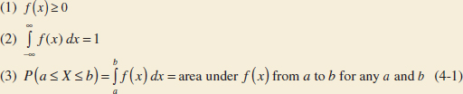
A probability density function provides a simple description of the probabilities associated with a random variable. As long as f(x) is nonnegative and ![]() f(x) = 1,0 ≤ P(a < X < b) ≤ 1 so that the probabilities are properly restricted. A probability density function is zero for x values that cannot occur, and it is assumed to be zero wherever it is not specifically defined.
f(x) = 1,0 ≤ P(a < X < b) ≤ 1 so that the probabilities are properly restricted. A probability density function is zero for x values that cannot occur, and it is assumed to be zero wherever it is not specifically defined.
A histogram is an approximation to a probability density function. See Fig. 4-3. For each interval of the histogram, the area of the bar equals the relative frequency (proportion) of the measurements in the interval. The relative frequency is an estimate of the probability that a measurement falls in the interval. Similarly, the area under f(x) over any interval equals the true probability that a measurement falls in the interval.
The important point is that f(x) is used to calculate an area that represents the probability that X assumes a value in [a,b]. For the current measurement example, the probability that X results in [14 mA, 15 mA] is the integral of the probability density function of X over this interval. The probability that X results in [14.5 mA, 14.6 mA] is the integral of the same function, f(x), over the smaller interval. By appropriate choice of the shape of f(x), we can represent the probabilities associated with any continuous random variable X. The shape of f(x) determines how the probability that X assumes a value in [14.5 mA, 14.6 mA] compares to the probability of any other interval of equal or different length.
For the density function of a loading on a long, thin beam, because every point has zero width, the loading at any point is zero. Similarly, for a continuous random variable X and any value x,
![]()
Based on this result, it might appear that our model of a continuous random variable is useless. However, in practice, when a particular current measurement such as 14.47 milliamperes, is observed, this result can be interpreted as the rounded value of a current measurement that is actually in a range such as 14.465 ≤ x ≤ 14.475. Therefore, the probability that the rounded value 14.47 is observed as the value for X is the probability that X assumes a value in the interval [14.465, 14.475], which is not zero. Similarly, because each point has zero probability, one need not distinguish between inequalities such as < or ≤ for continuous random variables.
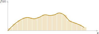
FIGURE 4-3 Histogram approximates a probability density function.
Example 4-1 Electric Current Let the continuous random variable X denote the current measured in a thin copper wire in milliamperes. Assume that the range of X is [4.9, 5.1]mA, and assume that the probability density function of X is f(x) = 5 for 4.9 ≤ x ≤ 5.1. What is the probability that a current measurement is less than 5 milliamperes?
The probability density function is shown in Fig. 4-4. It is assumed that f(x) = 0 wherever it is not specifically defined. The shaded area in Fig. 4-4 indicates the probability.
![]()
As another example,
![]()
Example 4-2 Hole Diameter Let the continuous random variable X denote the diameter of a hole drilled in a sheet metal component. The target diameter is 12.5 millimeters. Most random disturbances to the process result in larger diameters. Historical data show that the distribution of X can be modeled by a probability density function f(x) = 20e−20(x − 12.5), for x ≥ 12.5.
If a part with a diameter greater than 12.60 mm is scrapped, what proportion of parts is scrapped? The density function and the requested probability are shown in Fig. 4-5. A part is scrapped if X > 12.60. Now,

What proportion of parts is between 12.5 and 12.6 millimeters? Now
![]()
Because the total area under f(x) equals 1, we can also calculate P (12.5 < X < 12.6) = 1 − P(X > 12.6) = 1 − 0.135 = 0.865.
Practical Interpretation: Because 0.135 is the proportion of parts with diameters greater than 12.60 mm, a large proportion of parts is scrapped. Process improvements are needed to increase the proportion of parts with dimensions near 12.50 mm.

FIGURE 4-4 Probability density function for Example 4-1.

FIGURE 4-5 Probability density function for Example 4-2.
![]() Problem available in WileyPLUS at instructor's discretion.
Problem available in WileyPLUS at instructor's discretion.
![]() Go Tutorial Tutoring problem available in WileyPLUS at instructor's discretion.
Go Tutorial Tutoring problem available in WileyPLUS at instructor's discretion.
4-1. ![]() Suppose that f(x) = e−x for 0 < x. Determine the following:
Suppose that f(x) = e−x for 0 < x. Determine the following:
(a) P(1 < X)
(b) P(1 < X < 2.5)
(c) P(X = 3)
(d) P(X < 4)
(e) P(3 ≤ X)
(f) x such that P(x < X) = 0.10
(g) x such that P(X ≤ x) = 0.10
4-2. ![]() Suppose that f(x) = 3(8x − x2)/256 for 0 < x < 8. Determine the following:
Suppose that f(x) = 3(8x − x2)/256 for 0 < x < 8. Determine the following:
(a) P(X < 2)
(b) P(X < 9)
(c) P(2 < X < 4)
(d) P(X > 6)
(e) x such that P (X < x) = 0.95
4-3. Suppose that f(x) = 0.5 cos x for − π/2 < x < π/2. Determine the following:
(a) P(X < 0)
(b) P(X < − π/4)
(c) P(−π/4 < X < π/4)
(d) P(X > − π/4)
(e) x such that P(X < x) = 0.95
4-4. ![]() The diameter of a particle of contamination (in micrometers) is modeled with the probability density function f(x) = 2/x3 for x > 1. Determine the following:
The diameter of a particle of contamination (in micrometers) is modeled with the probability density function f(x) = 2/x3 for x > 1. Determine the following:
(a) P(X < 2)
(b) P(X > 5)
(c) P(4 < X < 8)
(d) P(X < 4 or X > 8)
(e) x such that P(X < x) = 0.95
4-5. ![]() Go Tutorial Suppose that f(x) = f(x) =
Go Tutorial Suppose that f(x) = f(x) = ![]() for 3 < x < 5. Determine the following probabilities:
for 3 < x < 5. Determine the following probabilities:
(a) P(X < 4)
(b) P(X > 3.5)
(c) P(4 < X < 5)
(d) P(X < 4.5)
(e) P(X < 3.5 or X > 4.5)
4-6. ![]() Suppose that f(x) = e−(x − 4) for 4 < x. Determine the following:
Suppose that f(x) = e−(x − 4) for 4 < x. Determine the following:
(a) P(1 < X)
(b) P(2 ≤ X < 5)
(c) P(5 < X)
(d) P(8 < X < 12)
(e) x such that P(X < x) = 0.90
4-7. ![]() Suppose that f(x) = 1.5x2 for − 1 < x < 1. Determine the following:
Suppose that f(x) = 1.5x2 for − 1 < x < 1. Determine the following:
(a) P(0 < X)
(b) P(0.5 < X)
(c) P(−0.5 ≤ X ≤ 0.5)
(d) P(X < −2)
(e) P(X < 0 or X > −0.5)
(f) x such that P(x < X) = 0.05.
4-8. ![]() The probability density function of the time to failure of an electronic component in a copier (in hours) is f(x) = e−x/1000/1000 for x > 0. Determine the probability that
The probability density function of the time to failure of an electronic component in a copier (in hours) is f(x) = e−x/1000/1000 for x > 0. Determine the probability that
(a) A component lasts more than 3000 hours before failure.
(b) A component fails in the interval from 1000 to 2000 hours.
(c) A component fails before 1000 hours.
(d) The number of hours at which 10% of all components have failed.
4-9. ![]() The probability density function of the net weight in pounds of a packaged chemical herbicide is f(x) = 2.0 for 49.75 < x < 50.25 pounds.
The probability density function of the net weight in pounds of a packaged chemical herbicide is f(x) = 2.0 for 49.75 < x < 50.25 pounds.
(a) Determine the probability that a package weighs more than 50 pounds.
(b) How much chemical is contained in 90% of all packages?
4-10. ![]() The probability density function of the length of a cutting blade is f(x) = 1.25 for 74.6 < x < 75.4 millimeters. Determine the following:
The probability density function of the length of a cutting blade is f(x) = 1.25 for 74.6 < x < 75.4 millimeters. Determine the following:
(a) P(X < 74.8)
(b) P(X < 74.8 or X > 75.2)
(c) If the specifications for this process are from 74.7 to 75.3 millimeters, what proportion of blades meets specifications?
4-11. ![]() The probability density function of the length of a metal rod is f(x) = 2 for 2.3 < x < 2.8 meters.
The probability density function of the length of a metal rod is f(x) = 2 for 2.3 < x < 2.8 meters.
(a) If the specifications for this process are from 2.25 to 2.75 meters, what proportion of rods fail to meet the specifications?
(b) Assume that the probability density function is f(x) = 2 for an interval of length 0.5 meters. Over what value should the density be centered to achieve the greatest proportion of rods within specifications?
4-12. An article in Electric Power Systems Research [“Modeling Real-Time Balancing Power Demands in Wind Power Systems Using Stochastic Differential Equations” (2010, Vol. 80(8), pp. 966–974)] considered a new probabilistic model to balance power demand with large amounts of wind power. In this model, the power loss from shutdowns is assumed to have a triangular distribution with probability density function
Determine the following:
(a) P(X < 90)
(b) P(100 < X ≤ 200)
(c) P(X > 800)
(d) Value exceeded with probability 0.1.
4-13. A test instrument needs to be calibrated periodically to prevent measurement errors. After some time of use without calibration, it is known that the probability density function of the measurement error is f(x) = 1 −0.5x for 0 < x < 2 millimeters.
(a) If the measurement error within 0.5 millimeters is acceptable, what is the probability that the error is not acceptable before calibration?
(b) What is the value of measurement error exceeded with probability 0.2 before calibration?
(c) What is the probability that the measurement error is exactly 0.22 millimeters before calibration?
4-14. The distribution of X is approximated with a triangular probability density function f(x) = 0.025x − 0.0375 for 30 < x < 50 and f(x) = −0.025x + 0.0875 for 50 < x < 70. Determine the following:
(a) P(X ≤ 40)
(b) P(40 < X ≤ 60)
(c) Value x exceeded with probability 0.99.
4-15. The waiting time for service at a hospital emergency department (in hours) follows a distribution with probability density function f(x) = 0.5 exp(−0.5x) for 0 < x. Determine the following:
(a) P(X < 0.5)
(b) P(X > 2)
(c) Value x (in hours) exceeded with probability 0.05.
4-16. If X is a continuous random variable, argue that P(x1 ≤ X ≤ x2) = P(x1 < X ≤ x2) = P(x1 ≤ X < x2) = P(x1 < X < x2).
4-3 Cumulative Distribution Functions
An alternative method to describe the distribution of a discrete random variable can also be used for continuous random variables.
Cumulative Distribution Function
The cumulative distribution function of a continuous random variable X is
![]()
for −∞ < x < ∞.
The cumulative distribution function is defined for all real numbers. The following example illustrates the definition.
Example 4-3 Electric Current For the copper current measurement in Example 4-1, the cumulative distribution function of the random variable X consists of three expressions. If x < 4.9, f(x) = 0. Therefore,
![]()
and
![]()
Finally,
![]()
Therefore,

The plot of F(x) is shown in Fig. 4-6.
Notice that in the definition of F(x), any < can be changed to ≤ and vice versa. That is, in Example 4-3 F(x) can be defined as either 5x − 24.5 or 0 at the end-point x = 4.9, and F(x) can be defined as either 5x − 24.5 or 1 at the end-point x = 5.1. In other words, F(x) is a continuous function. For a discrete random variable, F(x) is not a continuous function. Sometimes a continuous random variable is defined as one that has a continuous cumulative distribution function.

FIGURE 4-6 Cumulative distribution function for Example 4-3.
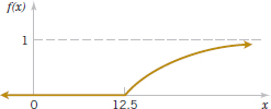
FIGURE 4-7 Cumulative distribution function for Example 4-4.
Example 4-4 Hole Diameter For the drilling operation in Example 4-2, F(x) consists of two expressions.
![]()
and for 12.5 ≤ x,
![]()
Therefore,
![]()
Figure 4-7 displays a graph of F(x).
Practical Interpretation: The cumulative distribution function enables one to easily calculate the probability a diameter in less than a value (such as 12.60 mm). Therefore, the probability of a scrapped part can be easily determined.
The probability density function of a continuous random variable can be determined from the cumulative distribution function by differentiating. The fundamental theorem of calculus states that
![]()
Probability Density Function from the Cumulative Distribution Function
Then, given F(x),
![]()
as long as the derivative exists.
Example 4-5 Reaction Time The time until a chemical reaction is complete (in milliseconds) is approximated by the cumulative distribution function
![]()
Determine the probability density function of X. What proportion of reactions is complete within 200 milliseconds? Using the result that the probability density function is the derivative of F(x), we obtain
![]()
The probability that a reaction completes within 200 milliseconds is
![]()
Exercises FOR SECTION 4-3
![]() Problem available in WileyPLUS at instructor's discretion.
Problem available in WileyPLUS at instructor's discretion.
![]() Go Tutorial Tutoring problem available in WileyPLUS at instructor's discretion.
Go Tutorial Tutoring problem available in WileyPLUS at instructor's discretion.
4-17. ![]() Suppose that the cumulative distribution function of the random variable X is
Suppose that the cumulative distribution function of the random variable X is

Determine the following:
(a) P(X < 2.8)
(b) P(X > 1.5)
(c) P(X < −2)
(d) P(X > 6)
4-18. ![]() Suppose that the cumulative distribution function of the random variable X is
Suppose that the cumulative distribution function of the random variable X is

Determine the following:
(a) P(X < 1.8)
(b) P(X > −1.5)
(c) P(X < −2)
(d) P(−1 < X < 1)
4-19. ![]() Determine the cumulative distribution function for the distribution in Exercise 4-1.
Determine the cumulative distribution function for the distribution in Exercise 4-1.
4-20. ![]() Determine the cumulative distribution function for the distribution in Exercise 4-2.
Determine the cumulative distribution function for the distribution in Exercise 4-2.
4-21. Determine the cumulative distribution function for the distribution in Exercise 4-3.
4-22. Determine the cumulative distribution function for the distribution in Exercise 4-4.
4-23. Determine the cumulative distribution function for the distribution in Exercise 4-5.
4-24. Determine the cumulative distribution function for the distribution in Exercise 4-8. Use the cumulative distribution function to determine the probability that a component lasts more than 3000 hours before failure.
4-25. Determine the cumulative distribution function for the distribution in Exercise 4-11. Use the cumulative distribution function to determine the probability that a length exceeds 2.7 meters.
4-26. ![]() The probability density function of the time you arrive at a terminal (in minutes after 8:00 A.M.) is f(x) = 0.1 exp(−0.1x) for 0 < x. Determine the probability that
The probability density function of the time you arrive at a terminal (in minutes after 8:00 A.M.) is f(x) = 0.1 exp(−0.1x) for 0 < x. Determine the probability that
(a) You arrive by 9:00 A.M.
(b) You arrive between 8:15 A.M. and 8:30 A.M.
(c) You arrive before 8:40 A.M. on two or more days of five days. Assume that your arrival times on different days are independent.
(d) Determine the cumulative distribution function and use the cumulative distribution function to determine the probability that you arrive between 8:15 A.M. and 8:30 A.M.
4-27. ![]() The gap width is an important property of a magnetic recording head. In coded units, if the width is a continuous random variable over the range from 0 < x < 2 with f(x) = 0.5x, determine the cumulative distribution function of the gap width.
The gap width is an important property of a magnetic recording head. In coded units, if the width is a continuous random variable over the range from 0 < x < 2 with f(x) = 0.5x, determine the cumulative distribution function of the gap width.
Determine the probability density function for each of the following cumulative distribution functions.
4-28. ![]() F(x) = 1 − e−2x x < 0
F(x) = 1 − e−2x x < 0
4-29. ![]()

4-30. ![]()

4-31. Determine the cumulative distribution function for the random variable in Exercise 4-13.
4-32. Determine the cumulative distribution function for the random variable in Exercise 4-14. Use the cumulative distribution function to determine the probability that the random variable is less than 55.
4-33. Determine the cumulative distribution function for the random variable in Exercise 4-15. Use the cumulative distribution function to determine the probability that 40 < X ≤ 60.
4-34. Determine the cumulative distribution function for the random variable in Exercise 4-16. Use the cumulative distribution function to determine the probability that the waiting time is less than one hour.
4-4 Mean and Variance of a Continuous Random Variable
The mean and variance can also be defined for a continuous random variable. Integration replaces summation in the discrete definitions. If a probability density function is viewed as a loading on a beam as in Fig. 4-1, the mean is the balance point.
Mean and Variance
Suppose that X is a continuous random variable with probability density function f(x). The mean or expected value of X, denoted as μ or E(X), is
![]()
The variance of X, denoted as V(X) or σ2, is
![]()
The standard deviation of X is σ = ![]() .
.
The equivalence of the two formulas for variance can be derived from the same approach used for discrete random variables.
Example 4-6 Electric Current For the copper current measurement in Example 4-1, the mean of X is
![]()
The variance of X is
![]()
The expected value of a function h(X) of a continuous random variable is also defined in a straightforward manner.
Expected Value of a Function of a Continuous Random Variable
If X is a continuous random variable with probability density function f(x),
![]()
In the special case that h(X) = aX + b for any constants a and b, E[h(X)] = aE(X) + b. This can be shown from the properties of integrals.
Example 4-7 In Example 4-1, X is the current measured in milliamperes. What is the expected value of power when the resistance is 100 ohms? Use the result that power in watts P = 10−6 RI2, where I is the current in milliamperes and R is the resistance in ohms. Now, h(X) = 10−6 100X2. Therefore,
![]()
Example 4-8 Hole Diameter For the drilling operation in Example 4-2, the mean of x is
![]()
Integration by parts can be used to show that
![]()
The variance of X is
![]()
Although more difficult, integration by parts can be used twice to show that V(X) = 0.0025 and σ = 0.05.
Practical Interpretation: The scrap limit at 12.60 mm is only 1 standard deviation greater than the mean. This is generally a warning that the scrap may be unacceptably high.
![]() Problem available in WileyPLUS at instructor's discretion.
Problem available in WileyPLUS at instructor's discretion.
![]() Go Tutorial Tutoring problem available in WileyPLUS at instructor's discretion.
Go Tutorial Tutoring problem available in WileyPLUS at instructor's discretion.
4-35. ![]() Suppose that f(x) = 0.25 for 0 < x < 4. Determine the mean and variance of X.
Suppose that f(x) = 0.25 for 0 < x < 4. Determine the mean and variance of X.
4-36. ![]() Suppose that f(x) = 0.125x for 0 < x < 4. Determine the mean and variance of X.
Suppose that f(x) = 0.125x for 0 < x < 4. Determine the mean and variance of X.
4-37. ![]() Suppose that f(x) = 1.5x2 for −1 < x < 1. Determine the mean and variance of X.
Suppose that f(x) = 1.5x2 for −1 < x < 1. Determine the mean and variance of X.
4-38. ![]() Suppose that f(x) = x/8 for 3 < x < 5. Determine the mean and variance of x.
Suppose that f(x) = x/8 for 3 < x < 5. Determine the mean and variance of x.
4-39. Determine the mean and variance of the random variable in Exercise 4-1.
4-40. Determine the mean and variance of the random variable in Exercise 4-2.
4-41. Determine the mean and variance of the random variable in Exercise 4-13.
4-42. Determine the mean and variance of the random variable in Exercise 4-14.
4-43. Determine the mean and variance of the random variable in Exercise 4-15.
4-44. Determine the mean and variance of the random variable in Exercise 4-16 .
4-45. ![]() Suppose that contamination particle size (in micrometers) can be modeled as f(x) = 2x−3 for 1 < x. Determine the mean of X. What can you conclude about the variance of X?
Suppose that contamination particle size (in micrometers) can be modeled as f(x) = 2x−3 for 1 < x. Determine the mean of X. What can you conclude about the variance of X?
4-46. ![]() Suppose that the probability density function of the length of computer cables is f(x) = 0.1 from 1200 to 1210 millimeters.
Suppose that the probability density function of the length of computer cables is f(x) = 0.1 from 1200 to 1210 millimeters.
(a) Determine the mean and standard deviation of the cable length.
(b) If the length specifications are 1195 < x < 1205 millimeters, what proportion of cables is within specifications?
4-47. ![]() The thickness of a conductive coating in micrometers has a density function of 600x− 2 for 100 μm < x < 120 μm.
The thickness of a conductive coating in micrometers has a density function of 600x− 2 for 100 μm < x < 120 μm.
(a) Determine the mean and variance of the coating thickness.
(b) If the coating costs $0.50 per micrometer of thickness on each part, what is the average cost of the coating per part?
4-48. ![]() The probability density function of the weight of packages delivered by a post office is f(x) = 70/(69x2) for 1 < x < 70 pounds.
The probability density function of the weight of packages delivered by a post office is f(x) = 70/(69x2) for 1 < x < 70 pounds.
(a) Determine the mean and variance of weight.
(b) If the shipping cost is $2.50 per pound, what is the average shipping cost of a package?
(c) Determine the probability that the weight of a package exceeds 50 pounds.
4-49. ![]() Integration by parts is required. The probability density function for the diameter of a drilled hole in millimeters is 10e−10(x−5) for x > 5 mm. Although the target diameter is 5 millimeters, vibrations, tool wear, and other nuisances produce diameters greater than 5 millimeters.
Integration by parts is required. The probability density function for the diameter of a drilled hole in millimeters is 10e−10(x−5) for x > 5 mm. Although the target diameter is 5 millimeters, vibrations, tool wear, and other nuisances produce diameters greater than 5 millimeters.
(a) Determine the mean and variance of the diameter of the holes.
(b) Determine the probability that a diameter exceeds 5.1 millimeters.
4-5 Continuous Uniform Distribution
The simplest continuous distribution is analogous to its discrete counterpart.
Continuous Uniform Distribution
A continuous random variable X with probability density function
![]()
is a continuous uniform random variable.
The probability density function of a continuous uniform random variable is shown in Fig. 4-8. The mean of the continuous uniform random variable X is
![]()
The variance of X is


FIGURE 4-8 Continuous uniform probability density function.

FIGURE 4-9 Probability for Example 4-9.
These results are summarized as follows.
Mean and Variance
If X is a continuous uniform random variable over a ≤ x ≤ b,
![]()
Example 4-9 Uniform Current In Example 4-1, the random variable X has a continuous uniform distribution on [4.9, 5.1]. The probability density function of X is f(x) = 5, 4.9 ≤ x ≤ 5.1.
What is the probability that a measurement of current is between 4.95 and 5.0 milliamperes? The requested probability is shown as the shaded area in Fig. 4-9.
![]()
The mean and variance formulas can be applied with a = 4.9 and b = 5.1. Therefore,
![]()
Consequently, the standard deviation of X is 0.0577 mA.
The cumulative distribution function of a continuous uniform random variable is obtained by integration. If a < x < b,
![]()
Therefore, the complete description of the cumulative distribution function of a continuous uniform random variable is

An example of F(x) for a continuous uniform random variable is shown in Fig. 4-6.
![]() Problem available in WileyPLUS at instructor's discretion.
Problem available in WileyPLUS at instructor's discretion.
![]() Go Tutorial Tutoring problem available in WileyPLUS at instructor's discretion.
Go Tutorial Tutoring problem available in WileyPLUS at instructor's discretion.
4-50. ![]() Suppose that X has a continuous uniform distribution over the interval [1.5, 5.5]. Determine the following:
Suppose that X has a continuous uniform distribution over the interval [1.5, 5.5]. Determine the following:
(a) Mean, variance, and standard deviation of X
(b) P(X < 2.5).
(c) Cumulative distribution function
4-51. ![]() Suppose X has a continuous uniform distribution over the interval [−1,1]. Determine the following:
Suppose X has a continuous uniform distribution over the interval [−1,1]. Determine the following:
(a) Mean, variance, and standard deviation of X
(b) Value for x such that P(−x < X < x) = 0.90
(c) Cumulative distribution function
4-52. ![]() The net weight in pounds of a packaged chemical herbicide is uniform for 49.75 < x < 50.25 pounds. Determine the following:
The net weight in pounds of a packaged chemical herbicide is uniform for 49.75 < x < 50.25 pounds. Determine the following:
(a) Mean and variance of the weight of packages
(b) Cumulative distribution function of the weight of packages
(c) P(X < 50.1)
4-53. ![]() The thickness of a flange on an aircraft component is uniformly distributed between 0.95 and 1.05 millimeters.
The thickness of a flange on an aircraft component is uniformly distributed between 0.95 and 1.05 millimeters.
Determine the following:
(a) Cumulative distribution function of flange thickness
(b) Proportion of flanges that exceeds 1.02 millimeters
(c) Thickness exceeded by 90% of the flanges
(d) Mean and variance of flange thickness
4-54. ![]() Suppose that the time it takes a data collection operator to fill out an electronic form for a database is uniformly between 1.5 and 2.2 minutes.
Suppose that the time it takes a data collection operator to fill out an electronic form for a database is uniformly between 1.5 and 2.2 minutes.
(a) What are the mean and variance of the time it takes an operator to fill out the form?
(b) What is the probability that it will take less than two minutes to fill out the form?
(c) Determine the cumulative distribution function of the time it takes to fill out the form.
4-55. ![]() The thickness of photoresist applied to wafers in semiconductor manufacturing at a particular location on the wafer is uniformly distributed between 0.2050 and 0.2150 micrometers. Determine the following:
The thickness of photoresist applied to wafers in semiconductor manufacturing at a particular location on the wafer is uniformly distributed between 0.2050 and 0.2150 micrometers. Determine the following:
(a) Cumulative distribution function of photoresist thickness
(b) Proportion of wafers that exceeds 0.2125 micrometers in photoresist thickness
(c) Thickness exceeded by 10% of the wafers
(d) Mean and variance of photoresist thickness
4-56. An adult can lose or gain two pounds of water in the course of a day. Assume that the changes in water weight are uniformly distributed between minus two and plus two pounds in a day. What is the standard deviation of a person's weight over a day?
4-57. ![]() A show is scheduled to start at 9:00 A.M., 9:30 A.M., and 10:00 A.M. Once the show starts, the gate will be closed. A visitor will arrive at the gate at a time uniformly distributed between 8:30 A.M. and 10:00 A.M. Determine the following:
A show is scheduled to start at 9:00 A.M., 9:30 A.M., and 10:00 A.M. Once the show starts, the gate will be closed. A visitor will arrive at the gate at a time uniformly distributed between 8:30 A.M. and 10:00 A.M. Determine the following:
(a) Cumulative distribution function of the time (in minutes) between arrival and 8:30 A.M.
(b) Mean and variance of the distribution in the previous part
(c) Probability that a visitor waits less than 10 minutes for a show
(d) Probability that a visitor waits more than 20 minutes for a show
4-58. The volume of a shampoo filled into a container is uniformly distributed between 374 and 380 milliliters.
(a) What are the mean and standard deviation of the volume of shampoo?
(b) What is the probability that the container is filled with less than the advertised target of 375 milliliters?
(c) What is the volume of shampoo that is exceeded by 95% of the containers?
(d) Every milliliter of shampoo costs the producer $0.002. Any shampoo more than 375 milliliters in the container is an extra cost to the producer. What is the mean extra cost?
4-59. An e-mail message will arrive at a time uniformly distributed between 9:00 A.M. and 11:00 A.M. You check e-mail at 9:15 A.M. and every 30 minutes afterward.
(a) What is the standard deviation of arrival time (in minutes)?
(b) What is the probability that the message arrives less than 10 minutes before you view it?
(c) What is the probability that the message arrives more than 15 minutes before you view it?
4-60. ![]() Measurement error that is continuous and uniformly distributed from −3 to +3 millivolts is added to a circuit's true voltage. Then the measurement is rounded to the nearest millivolt so that it becomes discrete. Suppose that the true voltage is 250 millivolts.
Measurement error that is continuous and uniformly distributed from −3 to +3 millivolts is added to a circuit's true voltage. Then the measurement is rounded to the nearest millivolt so that it becomes discrete. Suppose that the true voltage is 250 millivolts.
(a) What is the probability mass function of the measured voltage?
(b) What are the mean and variance of the measured voltage?
4-61. A beacon transmits a signal every 10 minutes (such as 8:20, 8:30, etc.). The time at which a receiver is tuned to detect the beacon is a continuous uniform distribution from 8:00 A.M. to 9:00 A.M. Consider the waiting time until the next signal from the beacon is received.
(a) Is it reasonable to model the waiting time as a continuous uniform distribution? Explain.
(b) What is the mean waiting time?
(c) What is the probability that the waiting time is less than 3 minutes?
4-62. An electron emitter produces electron beams with changing kinetic energy that is uniformly distributed between three and seven joules. Suppose that it is possible to adjust the upper limit of the kinetic energy (currently set to seven joules).
(a) What is the mean kinetic energy?
(b) What is the variance of the kinetic energy?
(c) What is the probability that an electron beam has a kinetic energy of exactly 3.2 joules?
(d) What should be the upper limit so that the mean kinetic energy increases to eight joules?
(e) What should be the upper limit so that the variance of kinetic energy decreases to 0.75 joules?
4-6 Normal Distribution
Undoubtedly, the most widely used model for a continuous measurement is a normal random variable. Whenever a random experiment is replicated, the random variable that equals the average (or total) result over the replicates tends to have a normal distribution as the number of replicates becomes large. De Moivre presented this fundamental result, known as the central limit theorem, in 1733. Unfortunately, his work was lost for some time, and Gauss independently developed a normal distribution nearly 100 years later. Although De Moivre was later credited with the derivation, a normal distribution is also referred to as a Gaussian distribution.
When do we average (or total) results? Almost always. For example, an automotive engineer may plan a study to average pull-off force measurements from several connectors. If we assume that each measurement results from a replicate of a random experiment, the normal distribution can be used to make approximate conclusions about this average. These conclusions are the primary topics in the subsequent chapters of this book.
Furthermore, sometimes the central limit theorem is less obvious. For example, assume that the deviation (or error) in the length of a machined part is the sum of a large number of infinitesimal effects, such as temperature and humidity drifts, vibrations, cutting angle variations, cutting tool wear, bearing wear, rotational speed variations, mounting and fixture variations, variations in numerous raw material characteristics, and variation in levels of contamination. If the component errors are independent and equally likely to be positive or negative, the total error can be shown to have an approximate normal distribution. Furthermore, the normal distribution arises in the study of numerous basic physical phenomena. For example, the physicist Maxwell developed a normal distribution from simple assumptions regarding the velocities of molecules.
The theoretical basis of a normal distribution is mentioned to justify the somewhat complex form of the probability density function. Our objective now is to calculate probabilities for a normal random variable. The central limit theorem will be stated more carefully in Chapter 5.
Random variables with different means and variances can be modeled by normal probability density functions with appropriate choices of the center and width of the curve. The value of E(X) = μ determines the center of the probability density function, and the value of V(X) = σ2 determines the width. Figure 4-10 illustrates several normal probability density functions with selected values of μ and σ2. Each has the characteristic symmetric bell-shaped curve, but the centers and dispersions differ. The following definition provides the formula for normal probability density functions.
Normal Distribution
A random variable X with probability density function
![]()
is a normal random variable with parameters μ where −∞ < μ < ∞, and σ > 0. Also,
![]()
and the notation N(μ, σ2) is used to denote the distribution.
The mean and variance of X are shown to equal μ and σ2, respectively, in an exercise at the end of Chapter 5.

FIGURE 4-10 Normal probability density functions for selected values of the parameters μ and σ2.

FIGURE 4-11 Probability that X > 13 for a normal random variable with μ = 10 and σ2 = 4.
Example 4-10 Assume that the current measurements in a strip of wire follow a normal distribution with a mean of 10 milliamperes and a variance of 4 (milliamperes)2. What is the probability that a measurement exceeds 13 milliamperes?
Let X denote the current in milliamperes. The requested probability can be represented as P(X > 13). This probability is shown as the shaded area under the normal probability density function in Fig. 4-11. Unfortunately, there is no closed-form expression for the integral of a normal probability density function, and probabilities based on the normal distribution are typically found numerically or from a table (that we introduce soon).
The following equations and Fig. 4-12 summarize some useful results concerning a normal distribution. For any normal random variable,

Also, from the symmetry of f(x), P(X < μ) = P(X < μ) = 0.5. Because f(x) is positive for all x, this model assigns some probability to each interval of the real line. However, the probability density function decreases as x moves farther from μ. Consequently, the probability that a measurement falls far from μ is small, and at some distance from μ, the probability of an interval can be approximated as zero.
The area under a normal probability density function beyond 3σ from the mean is quite small. This fact is convenient for quick, rough sketches of a normal probability density function. The sketches help us determine probabilities. Because more than 0.9973 of the probability of a normal distribution is within the interval (μ− 3σ, μ +3σ), 6σ is often referred to as the width of a normal distribution. Advanced integration methods can be used to show that the area under the normal probability density function from −∞ < x < ∞ is 1.
Standard Normal Random Variable
A normal random variable with
![]()
is called a standard normal random variable and is denoted as Z. The cumulative distribution function of a standard normal random variable is denoted as
![]()
Appendix Table III provides cumulative probabilities for a standard normal random variable. Cumulative distribution functions for normal random variables are also widely available in computer packages. They can be used in the same manner as Appendix Table III to obtain probabilities for these random variables. The use of Table III is illustrated by the following example.
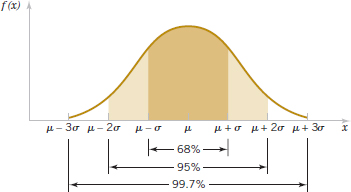
FIGURE 4-12 Probabilities associated with a normal distribution.
Example 4-11 Standard Normal Distribution Assume that Z is a standard normal random variable. Appendix Table III provides probabilities of the form Φ(z) = P(Z ≤ z). The use of Table III to find P(Z ≤ 1.5) is illustrated in Fig. 4-13. Read down the z column to the row that equals 1.5. The probability is read from the adjacent column, labeled 0.00, to be 0.93319.

FIGURE 4-13 Standard normal probability density function.
The column headings refer to the hundredths digit of the value of z in P(Z ≤ z). For example, P(Z ≤ 1.53) is found by reading down the z column to the row 1.5 and then selecting the probability from the column labeled 0.03 to be 0.93699.
Probabilities that are not of the form P(Z ≤ z) are found by using the basic rules of probability and the symmetry of the normal distribution along with Appendix Table III. The following examples illustrate the method.
Example 4-12 The following calculations are shown pictorially in Fig. 4-14. In practice, a probability is often rounded to one or two significant digits.
(1) P(Z > 1.26) = 1 − P(Z ≤ 1.26) = 1 − 0.89616 = = 0.10384.
(2) P(Z < 20.86) = 0.19490.
(3) P(Z > −1.37) = P(Z < 1.37) = 0.91465.
(4) P(−1.25 < Z < 0.37). This probability can be found from the difference of two areas, P(Z < 0.37) − P(Z < −1.25). Now,
![]()
and
![]()
Therefore,
![]()
(5) P(Z ≤ −4.6) cannot be found exactly from Appendix Table III. However, the last entry in the table can be used to find that P(Z ≤ −3.99) = 0.00003. Because P(Z ≤ −4.6) < P(Z ≤ −3.99), P(Z ≤ −4.6) is nearly zero.
(6) Find the value z such that P(Z > z) = 0.05. This probability expression can be written as P(Z ≤ z) = 0.95. Now Table III is used in reverse. We search through the probabilities to find the value that corresponds to 0.95. The solution is illustrated in Fig. 4-14. We do not find 0.95 exactly; the nearest value is 0.95053, corresponding to z = 1.65.
(7) Find the value of z such that P(−z < Z < z) = 0.99. Because of the symmetry of the normal distribution, if the area of the shaded region in Fig. 4-14(7) is to equal 0.99, the area in each tail of the distribution must equal 0.005. Therefore, the value for z corresponds to a probability of 0.995 in Table III. The nearest probability in Table III is 0.99506 when z = 2.58.
The cases in Example 4-12 show how to calculate probabilities for standard normal random variables. To use the same approach for an arbitrary normal random variable would require the availability of a separate table for every possible pair of values for μ and σ. Fortunately, all normal probability distributions are related algebraically, and Appendix Table III can be used to find the probabilities associated with an arbitrary normal random variable by first using a simple transformation.
Standardizing a Normal Random Variable
If X is a normal random variable with E(X) = μ and V(X) = σ2, the random variable
![]()
is a normal random variable with E(Z) = 0 and V(Z) = 1. That is, Z is a standard normal random variable.
Creating a new random variable by this transformation is referred to as standardizing. The random variable Z represents the distance of X from its mean in terms of standard deviations. It is the key step to calculating a probability for an arbitrary normal random variable.

FIGURE 4-14 Graphical displays for standard normal distributions.

FIGURE 4-15 Standardizing a normal random variable.
Example 4-13 Normally Distributed Current Suppose that the current measurements in a strip of wire are assumed to follow a normal distribution with a mean of 10 milliamperes and a variance of four (milliamperes)2. What is the probability that a measurement exceeds 13 milliamperes?
Let X denote the current in milliamperes. The requested probability can be represented as P(X > 13). Let Z = (X − 10)/2. The relationship between the several values of X and the transformed values of Z are shown in Fig. 4-15. We note that X > 13 corresponds to Z > 1.5. Therefore, from Appendix Table III,
![]()
Rather than using Fig. 4-15, the probability can be found from the inequality X > 13. That is,
![]()
Practical Interpretation: Probabilities for any normal random variable can be computed with a simple transform to a standard normal random variable.
In Example 4-13, the value 13 is transformed to 1.5 by standardizing, and 1.5 is often referred to as the z-value associated with a probability. The following summarizes the calculation of probabilities derived from normal random variables.
Standardizing to Calculate a Probability
Suppose that X is a normal random variable with mean μ and variance σ2. Then,
![]()
where Z is a standard normal random variable, and z = ![]() is the z-value obtained by standardizing X. The probability is obtained by using Appendix Table III with z = (x − μ)/σ.
is the z-value obtained by standardizing X. The probability is obtained by using Appendix Table III with z = (x − μ)/σ.

FIGURE 4-16 Determining the value of x to meet a specified probability.
Example 4-14 Normally Distributed Current Continuing Example 4-13, what is the probability that a current measurement is between 9 and 11 milliamperes? From Fig. 4-15, or by proceeding algebraically, we have

Determine the value for which the probability that a current measurement is less than this value is 0.98. The requested value is shown graphically in Fig. 4-16. We need the value of x such that P(X < x) = 0.98. By standardizing, this probability expression can be written as

Appendix Table III is used to find the z-value such that P(Z < z) = 0.98. The nearest probability from Table III results in
![]()
Therefore, (x −10)/2 = 2.05, and the standardizing transformation is used in reverse to solve for x. The result is
![]()
Example 4-15 Signal Detection Assume that in the detection of a digital signal, the background noise follows a normal distribution with a mean of 0 volt and standard deviation of 0.45 volt. The system assumes a digital 1 has been transmitted when the voltage exceeds 0.9. What is the probability of detecting a digital 1 when none was sent?
Let the random variable N denote the voltage of noise. The requested probability is
![]()
This probability can be described as the probability of a false detection.
Determine symmetric bounds about 0 that include 99% of all noise readings. The question requires us to find x such that P(−x < N < x) = 0.99. A graph is shown in Fig. 4-17. Now,
![]()
From Appendix Table III,
![]()
Therefore,
![]()
and
![]()
Suppose that when a digital 1 signal is transmitted, the mean of the noise distribution shifts to 1.8 volts. What is the probability that a digital 1 is not detected? Let the random variable S denote the voltage when a digital 1 is transmitted. Then,
![]()
This probability can be interpreted as the probability of a missed signal.
Practical Interpretation: Probability calculations such as these can be used to quantify the rates of missed signals or false signals and to select a threshold to distinguish a zero and a one bit.
Example 4-16 Shaft Diameter The diameter of a shaft in an optical storage drive is normally distributed with mean 0.2508 inch and standard deviation 0.0005 inch. The specifications on the shaft are 0.2500 ± 0.0015 inch. What proportion of shafts conforms to specifications?
Let X denote the shaft diameter in inches. The requested probability is shown in Fig. 4-18 and

Most of the nonconforming shafts are too large because the process mean is located very near to the upper specification limit. If the process is centered so that the process mean is equal to the target value of 0.2500,

Practical Interpretation: By recentering the process, the yield is increased to approximately 99.73%.

FIGURE 4-17 Determining the value of x to meet a specified probability.

FIGURE 4-18 Distribution for Example 4-16.
![]() Problem available in WileyPLUS at instructor's discretion.
Problem available in WileyPLUS at instructor's discretion.
![]() Go Tutorial Tutoring problem available in WileyPLUS at instructor's discretion.
Go Tutorial Tutoring problem available in WileyPLUS at instructor's discretion.
4-63. ![]() Use Appendix Table III to determine the following probabilities for the standard normal random variable Z:
Use Appendix Table III to determine the following probabilities for the standard normal random variable Z:
(a) P(Z < 1.32)
(b) P(Z < 3.0)
(c) P(Z > 1.45)
(d) P(Z > −2.15)
(e) P(−2.34 < Z < 1.76)
4-64. Use Appendix Table III to determine the following probabilities for the standard normal random variable Z:
(a) P(−1 < Z < 1)
(b) P(−2 < Z < 2)
(c) P(−3 < Z < 3)
(d) P(Z < 3)
(e) P(0 < Z < 1)
4-65. ![]() Assume that Z has a standard normal distribution. Use Appendix Table III to determine the value for z that solves each of the following:
Assume that Z has a standard normal distribution. Use Appendix Table III to determine the value for z that solves each of the following:
(a) P(Z < z) = 0.9
(b) P(Z < z) = 0.5
(c) P(Z > z) = 0.1
(d) P(Z > z) = 0.9
(e) P(−1.24 < Z < z) = 0.8
4-66. ![]() Assume that Z has a standard normal distribution. Use Appendix Table III to determine the value for z that solves each of the following:
Assume that Z has a standard normal distribution. Use Appendix Table III to determine the value for z that solves each of the following:
(a) P(−z < Z < z) = 0.95
(b) P(−z < Z < z) = 0.99
(c) P(−z < Z < z) = 0.68
(d) P(−z < Z < z) = 0.9973
4-67. ![]() Assume that X is normally distributed with a mean of 10 and a standard deviation of 2. Determine the following:
Assume that X is normally distributed with a mean of 10 and a standard deviation of 2. Determine the following:
(a) P(Z < 13)
(b) P(Z > 9)
(c) P(6 < X < 14)
(d) P(2 < X < 4)
(e) P(−2 < X < 8)
4-68. ![]() Assume that X is normally distributed with a mean of 10 and a standard deviation of 2. Determine the value for x that solves each of the following:
Assume that X is normally distributed with a mean of 10 and a standard deviation of 2. Determine the value for x that solves each of the following:
(a) P(X > x) = 0.5
(b) P(X > x) = 0.95
(c) P(x < X < 10) = 0.
(d) P(−x < X − 10 < x) = 0.95
(e) P(−x < X − 10 < x) = 0.99
4-69. ![]() Assume that X is normally distributed with a mean of 5 and a standard deviation of 4. Determine the following:
Assume that X is normally distributed with a mean of 5 and a standard deviation of 4. Determine the following:
(a) P(X < 11)
(b) P(X > 0)
(c) P(3 < X < 7)
(d) P(−2 < X < 9)
(e) P(2 < X < 8)
4-70. Assume that X is normally distributed with a mean of 5 and a standard deviation of 4. Determine the value for x that solves each of the following:
(a) P(X > x) = 0.5
(b) P(X > x) = 0.95
(c) P(x < X < 9) = 0.2
(d) P(3 < X < x) = 0.95
(e) P(−x < X − 5 < x) = 0.99
4-71. ![]() The compressive strength of samples of cement can be modeled by a normal distribution with a mean of 6000 kilograms per square centimeter and a standard deviation of 100 kilograms per square centimeter.
The compressive strength of samples of cement can be modeled by a normal distribution with a mean of 6000 kilograms per square centimeter and a standard deviation of 100 kilograms per square centimeter.
(a) What is the probability that a sample's strength is less than 6250 Kg/cm2?
(b) What is the probability that a sample's strength is between 5800 and 5900 Kg/cm2?
(c) What strength is exceeded by 95% of the samples?
4-72. ![]() The time until recharge for a battery in a laptop computer under common conditions is normally distributed with a mean of 260 minutes and a standard deviation of 50 minutes.
The time until recharge for a battery in a laptop computer under common conditions is normally distributed with a mean of 260 minutes and a standard deviation of 50 minutes.
(a) What is the probability that a battery lasts more than four hours?
(b) What are the quartiles (the 25% and 75% values) of battery life?
(c) What value of life in minutes is exceeded with 95% probability?
4-73. An article in Knee Surgery Sports Traumatol Arthrosc [“Effect of Provider Volume on Resource Utilization for Surgical Procedures” (2005, Vol. 13, pp. 273–279)] showed a mean time of 129 minutes and a standard deviation of 14 minutes for anterior cruciate ligament (ACL) reconstruction surgery at high-volume hospitals (with more than 300 such surgeries per year).
(a) What is the probability that your ACL surgery at a high-volume hospital requires a time more than two standard deviations above the mean?
(b) What is the probability that your ACL surgery at a high-volume hospital is completed in less than 100 minutes?
(c) The probability of a completed ACL surgery at a high-volume hospital is equal to 95% at what time?
(d) If your surgery requires 199 minutes, what do you conclude about the volume of such surgeries at your hospital? Explain.
4-74. Cholesterol is a fatty substance that is an important part of the outer lining (membrane) of cells in the body of animals. Its normal range for an adult is 120–240 mg/dl. The Food and Nutrition Institute of the Philippines found that the total cholesterol level for Filipino adults has a mean of 159.2 mg/dl and 84.1% of adults have a cholesterol level less than 200 mg/dl (http://www.fnri.dost.gov.ph/). Suppose that the total cholesterol level is normally distributed.
(a) Determine the standard deviation of this distribution.
(b) What are the quartiles (the 25% and 75% percentiles) of this distribution?
(c) What is the value of the cholesterol level that exceeds 90% of the population?
(d) An adult is at moderate risk if cholesterol level is more than one but less than two standard deviations above the mean. What percentage of the population is at moderate risk according to this criterion?
(e) An adult whose cholesterol level is more than two standard deviations above the mean is thought to be at high risk. What percentage of the population is at high risk?
(f) An adult whose cholesterol level is less than one standard deviations below the mean is thought to be at low risk. What percentage of the population is at low risk?
4-75. ![]() The line width for semiconductor manufacturing is assumed to be normally distributed with a mean of 0.5 micrometer and a standard deviation of 0.05 micrometer.
The line width for semiconductor manufacturing is assumed to be normally distributed with a mean of 0.5 micrometer and a standard deviation of 0.05 micrometer.
(a) What is the probability that a line width is greater than 0.62 micrometer?
(b) What is the probability that a line width is between 0.47 and 0.63 micrometer?
(c) The line width of 90% of samples is below what value?
4-76. ![]() The fill volume of an automated filling machine used for filling cans of carbonated beverage is normally distributed with a mean of 12.4 fluid ounces and a standard deviation of 0.1 fluid ounce.
The fill volume of an automated filling machine used for filling cans of carbonated beverage is normally distributed with a mean of 12.4 fluid ounces and a standard deviation of 0.1 fluid ounce.
(a) What is the probability that a fill volume is less than 12 fluid ounces?
(b) If all cans less than 12.1 or more than 12.6 ounces are scrapped, what proportion of cans is scrapped?
(c) Determine specifications that are symmetric about the mean that include 99% of all cans.
4-77. In the previous exercise, suppose that the mean of the filling operation can be adjusted easily, but the standard deviation remains at 0.1 fluid ounce.
(a) At what value should the mean be set so that 99.9% of all cans exceed 12 fluid ounces?
(b) At what value should the mean be set so that 99.9% of all cans exceed 12 fluid ounces if the standard deviation can be reduced to 0.05 fluid ounce?
4-78. ![]() A driver's reaction time to visual stimulus is normally distributed with a mean of 0.4 seconds and a standard deviation of 0.05 seconds.
A driver's reaction time to visual stimulus is normally distributed with a mean of 0.4 seconds and a standard deviation of 0.05 seconds.
(a) What is the probability that a reaction requires more than 0.5 seconds?
(b) What is the probability that a reaction requires between 0.4 and 0.5 seconds?
(c) What reaction time is exceeded 90% of the time?
4-79. The speed of a file transfer from a server on campus to a personal computer at a student's home on a weekday evening is normally distributed with a mean of 60 kilobits per second and a standard deviation of four kilobits per second.
(a) What is the probability that the file will transfer at a speed of 70 kilobits per second or more?
(b) What is the probability that the file will transfer at a speed of less than 58 kilobits per second?
(c) If the file is one megabyte, what is the average time it will take to transfer the file? (Assume eight bits per byte.)
4-80. In 2002, the average height of a woman aged 20–74 years was 64 inches with an increase of approximately 1 inch from 1960 (http://usgovinfo.about.com/od/healthcare). Suppose the height of a woman is normally distributed with a standard deviation of two inches.
(a) What is the probability that a randomly selected woman in this population is between 58 inches and 70 inches?
(b) What are the quartiles of this distribution?
(c) Determine the height that is symmetric about the mean that includes 90% of this population.
(d) What is the probability that five women selected at random from this population all exceed 68 inches?
4-81. In an accelerator center, an experiment needs a 1.41-cm-thick aluminum cylinder (http://puhep1.princeton.edu/mumu/target/Solenoid_Coil.pdf). Suppose that the thickness of a cylinder has a normal distribution with a mean of 1.41 cm and a standard deviation of 0.01 cm.
(a) What is the probability that a thickness is greater than 1.42 cm?
(b) What thickness is exceeded by 95% of the samples?
(c) If the specifications require that the thickness is between 1.39 cm and 1.43 cm, what proportion of the samples meets specifications?
4-82. ![]() Go Tutorial The demand for water use in Phoenix in 2003 hit a high of about 442 million gallons per day on June 27 (http://phoenix.gov/WATER/wtrfacts.html). Water use in the summer is normally distributed with a mean of 310 million gallons per day and a standard deviation of 45 million gallons per day. City reservoirs have a combined storage capacity of nearly 350 million gallons.
Go Tutorial The demand for water use in Phoenix in 2003 hit a high of about 442 million gallons per day on June 27 (http://phoenix.gov/WATER/wtrfacts.html). Water use in the summer is normally distributed with a mean of 310 million gallons per day and a standard deviation of 45 million gallons per day. City reservoirs have a combined storage capacity of nearly 350 million gallons.
(a) What is the probability that a day requires more water than is stored in city reservoirs?
(b) What reservoir capacity is needed so that the probability that it is exceeded is 1%?
(c) What amount of water use is exceeded with 95% probability?
(d) Water is provided to approximately 1.4 million people. What is the mean daily consumption per person at which the probability that the demand exceeds the current reservoir capacity is 1%? Assume that the standard deviation of demand remains the same.
4-83. The life of a semiconductor laser at a constant power is normally distributed with a mean of 7000 hours and a standard deviation of 600 hours.
(a) What is the probability that a laser fails before 5000 hours?
(b) What is the life in hours that 95% of the lasers exceed?
(c) If three lasers are used in a product and they are assumed to fail independently, what is the probability that all three are still operating after 7000 hours?
4-84. The diameter of the dot produced by a printer is normally distributed with a mean diameter of 0.002 inch and a standard deviation of 0.0004 inch.
(a) What is the probability that the diameter of a dot exceeds 0.0026?
(b) What is the probability that a diameter is between 0.0014 and 0.0026?
(c) What standard deviation of diameters is needed so that the probability in part (b) is 0.995?
4-85. The weight of a sophisticated running shoe is normally distributed with a mean of 12 ounces and a standard deviation of 0.5 ounce.
(a) What is the probability that a shoe weighs more than 13 ounces?
(b) What must the standard deviation of weight be in order for the company to state that 99.9% of its shoes weighs less than 13 ounces?
(c) If the standard deviation remains at 0.5 ounce, what must the mean weight be for the company to state that 99.9% of its shoes weighs less than 13 ounces?
4-86. Measurement error that is normally distributed with a mean of 0 and a standard deviation of 0.5 gram is added to the true weight of a sample. Then the measurement is rounded to the nearest gram. Suppose that the true weight of a sample is 165.5 grams.
(a) What is the probability that the rounded result is 167 grams?
(b) What is the probability that the rounded result is 167 grams or more?
4-87. Assume that a random variable is normally distributed with a mean of 24 and a standard deviation of 2. Consider an interval of length one unit that starts at the value a so that the interval is[a,a + 1]. For what value of a is the probability of the interval greatest? Does the standard deviation affect that choice of interval?
4-88. A study by Bechtel et al., 2009, described in the Archives of Environmental & Occupational Health considered polycyclic aromatic hydrocarbons and immune system function in beef cattle. Some cattle were near major oil- and gas-producing areas of western Canada. The mean monthly exposure to PM 1.0 (particulate matter that is < 1 μm in diameter) was approximately 7.1 μg/m3 with standard deviation 1.5. Assume that the monthly exposure is normally distributed.
(a) What is the probability of a monthly exposure greater than 9 μg/m3?
(b) What is the probability of a monthly exposure between 3 and 8 μg/m3?
(c) What is the monthly exposure level that is exceeded with probability 0.05?
(d) What value of mean monthly exposure is needed so that the probability of a monthly exposure more than 9 μg/m3 is 0.01?
4-89. An article in Atmospheric Chemistry and Physics “Relationship Between Particulate Matter and Childhood Asthma—Basis of a Future Warning System for Central Phoenix” (2012, Vol. 12, pp. 2479–2490)] reported the use of PM10 (particulate matter < 10 μm diameter) air quality data measured hourly from sensors in Phoenix, Arizona. The 24-hour (daily) mean PM10 for a centrally located sensor was 50.9 μg/m3 with a standard deviation of 25.0. Assume that the daily mean of PM10 is normally distributed.
(a) What is the probability of a daily mean of PM10 greater than 100 μg/m3?
(b) What is the probability of a daily mean of PM10 less than 25 μg/m3?
(c) What daily mean of PM10 value is exceeded with probability 5%?
4-90. The length of stay at a specific emergency department in Phoenix, Arizona, in 2009 had a mean of 4.6 hours with a standard deviation of 2.9. Assume that the length of stay is normally distributed.
(a) What is the probability of a length of stay greater than 10 hours?
(b) What length of stay is exceeded by 25% of the visits?
(c) From the normally distributed model, what is the probability of a length of stay less than 0 hours? Comment on the normally distributed assumption in this example.
4-91. A signal in a communication channel is detected when the voltage is higher than 1.5 volts in absolute value. Assume that the voltage is normally distributed with a mean of 0. What is the standard deviation of voltage such that the probability of a false signal is 0.005?
4-92. An article in Microelectronics Reliability [“Advanced Electronic Prognostics through System Telemetry and Pattern Recognition Methods” (2007, Vol. 47(12), pp. 1865–1873)] presented an example of electronic prognosis. The objective was to detect faults to decrease the system downtime and the number of unplanned repairs in high-reliability systems. Previous measurements of the power supply indicated that the signal is normally distributed with a mean of 1.5 V and a standard deviation of 0.02 V.
(a) Suppose that lower and upper limits of the predetermined specifications are 1.45 V and 1.55 V, respectively. What is the probability that a signal is within these specifications?
(b) What is the signal value that is exceeded with 95% probability?
(c) What is the probability that a signal value exceeds the mean by two or more standard deviations?
4-93. An article in International Journal of Electrical Power & Energy Systems [“Stochastic Optimal Load Flow Using a Combined Quasi–Newton and Conjugate Gradient Technique” (1989, Vol. 11(2), pp. 85–93)] considered the problem of optimal power flow in electric power systems and included the effects of uncertain variables in the problem formulation. The method treats the system power demand as a normal random variable with 0 mean and unit variance.
(a) What is the power demand value exceeded with 95% probability?
(b) What is the probability that the power demand is positive?
(c) What is the probability that the power demand is more than – 1 and less than 1?
4-94. An article in the Journal of Cardiovascular Magnetic Resonance [“Right Ventricular Ejection Fraction Is Better Reflected by Transverse Rather Than Longitudinal Wall Motion in Pulmonary Hypertension” (2010, Vol. 12(35)] discussed a study of the regional right ventricle transverse wall motion in patients with pulmonary hypertension (PH). The right ventricle ejection fraction (EF) was approximately normally distributed with a mean and a standard deviation of 36 and 12, respectively, for PH subjects, and with mean and standard deviation of 56 and 8, respectively, for control subjects.
(a) What is the EF for PH subjects exceeded with 5% probability?
(b) What is the probability that the EF of a control subject is less than the value in part (a)?
(c) Comment on how well the control and PH subjects can be distinguished by EF measurements.
4-7 Normal Approximation to the Binomial and Poisson Distributions
We began our section on the normal distribution with the central limit theorem and the normal distribution as an approximation to a random variable with a large number of trials. Consequently, it should not be surprising to learn that the normal distribution can be used to approximate binomial probabilities for cases in which n is large. The following example illustrates that for many physical systems, the binomial model is appropriate with an extremely large value for n. In these cases, it is difficult to calculate probabilities by using the binomial distribution. Fortunately, the normal approximation is most effective in these cases. An illustration is provided in Fig. 4-19. The area of each bar equals the binomial probability of x. Notice that the area of bars can be approximated by areas under the normal probability density function.
From Fig. 4-19, it can be seen that a probability such as P(3 ≤ X ≤ 7) is better approximated by the area under the normal curve from 2.5 to 7.5. Consequently, a modified interval is used to better compensate for the difference between the continuous normal distribution and the discrete binomial distribution. This modification is called a continuity correction.
Example 4-17 Assume that in a digital communication channel, the number of bits received in error can be modeled by a binomial random variable, and assume that the probability that a bit is received in error is 1× 10⁻⁵. If 16 million bits are transmitted, what is the probability that 150 or fewer errors occur?
Let the random variable X denote the number of errors. Then X is a binomial random variable and
![]()
Practical Interpretation: Clearly, this probability is difficult to compute. Fortunately, the normal distribution can be used to provide an excellent approximation in this example.
Normal Approximation to the Binomial Distribution
If X is a binomial random variable with parameters n and p,
![]()
is approximately a standard normal random variable. To approximate a binomial probability with a normal distribution, a continuity correction is applied as follows:

and

The approximation is good for np > 5 and n(1 − p) > 5.
Recall that for a binomial variable X, E(X) = np and V(X) = np(1 − p). Consequently, the expression in Equation 4-12 is nothing more than the formula for standardizing the random variable X. Probabilities involving X can be approximated by using a standard normal distribution. The approximation is good when n is large relative to p.
A way to remember the approximation is to write the probability in terms of ≤ or ≥ and then add or subtract the 0.5 correction factor to make the probability greater.

FIGURE 4-19 Normal approximation to the binomial distribution.

FIGURE 4-20 Binomial distribution is not symmetrical if p is near 0 or 1.
Example 4-18 The digital communication problem in Example 4-17 is solved as follows:

Because np = (16 × 106)(1 ×10⁻⁵) = 160 and n(1 − p) is much larger, the approximation is expected to work well in this case.
Practical Interpretation: Binomial probabilities that are difficult to compute exactly can be approximated with easy-to-compute probabilities based on the normal distribution.
Example 4-19 Normal Approximation to Binomial Again consider the transmission of bits in Example 4-18. To judge how well the normal approximation works, assume that only n = 50 bits are to be transmitted and that the probability of an error is p = 0.1. The exact probability that two or fewer errors occur is
![]()
Based on the normal approximation,

As another example, P(8 < X) = P(9 ≤ X), which is better approximated as
![]()
We can even approximate P(X = 5) = P(5 ≤ X ≤ 5) as
and this compares well with the exact answer of 0.1849.
Practical Interpretation: Even for a sample as small as 50 bits, the normal approximation is reasonable, when p = 0.1.
The correction factor is used to improve the approximation. However, if np or n(1 − p) is small, the binomial distribution is quite skewed and the symmetric normal distribution is not a good approximation. Two cases are illustrated in Fig. 4-20.
Recall that the binomial distribution is a satisfactory approximation to the hypergeometric distribution when n, the sample size, is small relative to N, the size of the population from which the sample is selected. A rule of thumb is that the binomial approximation is effective if n/N < 0.1. Recall that for a hypergeometric distribution, p is defined as p = K/N. That is, p is interpreted as the number of successes in the population. Therefore, the normal distribution can provide an effective approximation of hypergeometric probabilities when n/N < 0.1, np > 5, and n(1 − p) > 5. Figure 4-21 provides a summary of these guidelines.
Recall that the Poisson distribution was developed as the limit of a binomial distribution as the number of trials increased to infinity. Consequently, it should not be surprising to find that the normal distribution can also be used to approximate probabilities of a Poisson random variable.
Normal Approximation to the Poisson Distribution
If X is a Poisson random variable with E(X) = λ and V(X) = λ,
![]()
is approximately a standard normal random variable. The same continuity correction used for the binomial distribution can also be applied. The approximation is good for
λ > 5
Example 4-20 Normal Approximation to Poisson Assume that the number of asbestos particles in a squared meter of dust on a surface follows a Poisson distribution with a mean of 1000. If a squared meter of dust is analyzed, what is the probability that 950 or fewer particles are found?
This probability can be expressed exactly as
![]()
The computational difficulty is clear. The probability can be approximated as
![]()
Practical Interpretation: Poisson probabilities that are difficult to compute exactly can be approximated with easy-to-compute probabilities based on the normal distribution.
![]()
FIGURE 4-21 Conditions for approximating hypergeometric and binomial probabilities.
![]() Problem available in WileyPLUS at instructor's discretion.
Problem available in WileyPLUS at instructor's discretion.
![]() Go Tutorial Tutoring problem available in WileyPLUS at instructor's discretion.
Go Tutorial Tutoring problem available in WileyPLUS at instructor's discretion.
4-95. ![]() Suppose that X is a binomial random variable with n = 200 and p = 0.4. Approximate the following probabilities:
Suppose that X is a binomial random variable with n = 200 and p = 0.4. Approximate the following probabilities:
(a) P(X ≤ 70)
(b) P(70 < X < 90)
(c) P(X = 80)
4-96. ![]() Suppose that X is a Poisson random variable with λ = 6.
Suppose that X is a Poisson random variable with λ = 6.
(a) Compute the exact probability that X is less than four.
(b) Approximate the probability that X is less than four and compare to the result in part (a).
(c) Approximate the probability that 8 < X < 12.
4-97. ![]() Suppose that X has a Poisson distribution with a mean of 64. Approximate the following probabilities:
Suppose that X has a Poisson distribution with a mean of 64. Approximate the following probabilities:
(a) P(X > 72)
(b) P(X < 64)
(c) P(60 < X ≤ 68)
4-98. ![]() The manufacturing of semiconductor chips produces 2% defective chips. Assume that the chips are independent and that a lot contains 1000 chips. Approximate the following probabilities:
The manufacturing of semiconductor chips produces 2% defective chips. Assume that the chips are independent and that a lot contains 1000 chips. Approximate the following probabilities:
(a) More than 25 chips are defective.
(b) Between 20 and 30 chips are defective.
4-99. ![]() There were 49.7 million people with some type of long-lasting condition or disability living in the United States in 2000. This represented 19.3 percent of the majority of civilians aged five and over (http://factfinder.census.gov). A sample of 1000 persons is selected at random.
There were 49.7 million people with some type of long-lasting condition or disability living in the United States in 2000. This represented 19.3 percent of the majority of civilians aged five and over (http://factfinder.census.gov). A sample of 1000 persons is selected at random.
(a) Approximate the probability that more than 200 persons in the sample have a disability.
(b) Approximate the probability that between 180 and 300 people in the sample have a disability.
4-100. Phoenix water is provided to approximately 1.4 million people who are served through more than 362,000 accounts (http://phoenix.gov/WATER/wtrfacts.html). All accounts are metered and billed monthly. The probability that an account has an error in a month is 0.001, and accounts can be assumed to be independent.
(a) What are the mean and standard deviation of the number of account errors each month?
(b) Approximate the probability of fewer than 350 errors in a month.
(c) Approximate a value so that the probability that the number of errors exceeds this value is 0.05.
(d) Approximate the probability of more than 400 errors per month in the next two months. Assume that results between months are independent.
4-101. ![]() An electronic office product contains 5000 electronic components. Assume that the probability that each component operates without failure during the useful life of the product is 0.999, and assume that the components fail independently. Approximate the probability that 10 or more of the original 5000 components fail during the useful life of the product.
An electronic office product contains 5000 electronic components. Assume that the probability that each component operates without failure during the useful life of the product is 0.999, and assume that the components fail independently. Approximate the probability that 10 or more of the original 5000 components fail during the useful life of the product.
4-102. ![]() A corporate Web site contains errors on 50 of 1000 pages. If 100 pages are sampled randomly without replacement, approximate the probability that at least one of the pages in error is in the sample.
A corporate Web site contains errors on 50 of 1000 pages. If 100 pages are sampled randomly without replacement, approximate the probability that at least one of the pages in error is in the sample.
4-103. ![]() Suppose that the number of asbestos particles in a sample of 1 squared centimeter of dust is a Poisson random variable with a mean of 1000. What is the probability that 10 squared centimeters of dust contains more than 10,000 particles?
Suppose that the number of asbestos particles in a sample of 1 squared centimeter of dust is a Poisson random variable with a mean of 1000. What is the probability that 10 squared centimeters of dust contains more than 10,000 particles?
4-104. ![]() A high-volume printer produces minor print-quality errors on a test pattern of 1000 pages of text according to a Poisson distribution with a mean of 0.4 per page.
A high-volume printer produces minor print-quality errors on a test pattern of 1000 pages of text according to a Poisson distribution with a mean of 0.4 per page.
(a) Why are the numbers of errors on each page independent random variables?
(b) What is the mean number of pages with errors (one or more)?
(c) Approximate the probability that more than 350 pages contain errors (one or more).
4-105. Hits to a high-volume Web site are assumed to follow a Poisson distribution with a mean of 10,000 per day. Approximate each of the following:
(a) Probability of more than 20,000 hits in a day
(b) Probability of less than 9900 hits in a day
(c) Value such that the probability that the number of hits in a day exceeds the value is 0.01
(d) Expected number of days in a year (365 days) that exceed 10,200 hits.
(e) Probability that over a year (365 days), each of the more than 15 days has more than 10,200 hits.
4-106. An acticle in Biometrics [“Integrative Analysis of Transcriptomic and Proteomic Data of Desulfovibrio Vulgaris: A Nonlinear Model to Predict Abundance of Undetected Proteins” (2009)] reported that protein abundance from an operon (a set of biologically related genes) was less dispersed than from randomly selected genes. In the research, 1000 sets of genes were randomly constructed, and of these sets, 75% were more disperse than a specific opteron. If the probability that a random set is more disperse than this opteron is truly 0.5, approximate the probability that 750 or more random sets exceed the opteron. From this result, what do you conclude about the dispersion in the opteron versus random genes?
4-107. An article in Atmospheric Chemistry and Physics [“Relationship Between Particulate Matter and Childhood Asthma – Basis of a Future Warning System for Central Phoenix,” 2012, Vol. 12, pp. 2479-2490] linked air quality to childhood asthma incidents. The study region in central Phoenix, Arizona recorded 10,500 asthma incidents in children in a 21-month period. Assume that the number of asthma incidents follows a Poisson distribution.
(a) Approximate the probability of more than 550 asthma incidents in a month.
(b) Approximate the probability of 450 to 550 asthma incidents in a month.
(c) Approximate the number of asthma incidents exceeded with probability 5%.
(d) If the number of asthma incidents was greater during the winter than the summer, what would this imply about the Poisson distribution assumption?
4-108. A set of 200 independent patients take antiacid medication at the start of symptoms, and 80 experience moderate to substantial relief within 90 minutes. Historically, 30% of patients experience relief within 90 minutes with no medication. If the medication has no effect, approximate the probability that 80 or more patients experience relief of symptoms. What can you conclude about the effectiveness of this medication?
4-109. Among homeowners in a metropolitan area, 75% recycle plastic bottles each week. A waste management company services 1500 homeowners (assumed independent). Approximate the following probabilities:
(a) At least 1150 recycle plastic bottles in a week
(b) Between 1075 and 1175 recycle plastic bottles in a week
4-110. Cabs pass your workplace according to a Poisson process with a mean of five cabs per hour.
(a) Determine the mean and standard deviation of the number of cabs per 10-hour day.
(b) Approximate the probability that more than 65 cabs pass within a 10-hour day.
(c) Approximate the probability that between 50 and 65 cabs pass in a 10-hour day.
(d) Determine the mean hourly rate so that the probability is approximately 0.95 that 100 or more cabs pass in a 10-hour data.
4-111. The number of (large) inclusions in cast iron follows a Poisson distribution with a mean of 2.5 per cubic millimeter. Approximate the following probabilities:
(a) Determine the mean and standard deviation of the number of inclusions in a cubic centimeter (cc).
(b) Approximate the probability that fewer than 2600 inclusions occur in a cc.
(c) Approximate the probability that more than 2400 inclusions occur in a cc.
(d) Determine the mean number of inclusions per cubic millimeter such that the probability is approximately 0.9 that 500 or fewer inclusions occur in a cc.
4-8 Exponential Distribution
The discussion of the Poisson distribution defined a random variable to be the number of flaws along a length of copper wire. The distance between flaws is another random variable that is often of interest. Let the random variable X denote the length from any starting point on the wire until a flaw is detected. As you might expect, the distribution of X can be obtained from knowledge of the distribution of the number of flaws. The key to the relationship is the following concept. The distance to the first flaw exceeds three millimeters if and only if there are no flaws within a length of three millimeters—simple but sufficient for an analysis of the distribution of X.
In general, let the random variable N denote the number of flaws in x millimeters of wire. If the mean number of flaws is λ per millimeter, N has a Poisson distribution with mean λx. We assume that the wire is longer than the value of x. Now
![]()
Therefore,
![]()
is the cumulative distribution function of X. By differentiating F(x), the probability density function of X is calculated to be
![]()
The derivation of the distribution of X depends only on the assumption that the flaws in the wire follow a Poisson process. Also, the starting point for measuring X does not matter because the probability of the number of flaws in an interval of a Poisson process depends only on the length of the interval, not on the location. For any Poisson process, the following general result applies.
Exponential Distribution
The random variable X that equals the distance between successive events from a Poisson process with mean number of events λ > 0 per unit interval is an exponential random variable with parameter λ. The probability density function of X is
![]()
The exponential distribution obtains its name from the exponential function in the probability density function. See plots of the exponential distribution for selected values of λ in Fig. 4-22. For any value of λ, the exponential distribution is quite skewed. The following results are easily obtained and are left as an exercise.

FIGURE 4-22 Probability density function of exponential random variables for selected values of λ.

FIGURE 4-23 Probability for the exponential distribution in Example 4-21.
Mean and Variance
If the random variable X has an exponential distribution with parameter λ,
![]()
It is important to use consistent units to express intervals, X, and λ. The following example illustrates unit conversions.
Example 4-21 Computer Usage In a large corporate computer network, user log-ons to the system can be modeled as a Poisson process with a mean of 25 log-ons per hour. What is the probability that there are no log-ons in an interval of six minutes?
Let X denote the time in hours from the start of the interval until the first log-on. Then X has an exponential distribution with λ = 25 log-ons per hour. We are interested in the probability that X exceeds 6 minutes. Because λ is given in log-ons per hour, we express all time units in hours. That is, 6 minutes = 0.1 hour. The probability requested is shown as the shaded area under the probability density function in Fig. 4-23. Therefore,
![]()
The cumulative distribution function also can be used to obtain the same result as follows:
![]()
An identical answer is obtained by expressing the mean number of log-ons as 0.417 log-ons per minute and computing the probability that the time until the next log-on exceeds six minutes. Try it.
What is the probability that the time until the next log-on is between two and three minutes? Upon converting all units to hours,
An alternative solution is
![]()
Determine the interval of time such that the probability that no log-on occurs in the interval is 0.90. The question asks for the length of time x such that P(X > x) = 0.90. Now,
![]()
Take the (natural) log of both sides to obtain −25x = ln(0.90) = −0.1054. Therefore,
![]()
Furthermore, the mean time until the next log-on is
![]()
The standard deviation of the time until the next log-on is
![]()
Practical Interpretation: Organizations make wide use of probabilities for exponential random variables to evaluate resources and staffing levels to meet customer service needs.
In Example 4-21, the probability that there are no log-ons in a six-minute interval is 0.082 regardless of the starting time of the interval. A Poisson process assumes that events occur uniformly throughout the interval of observation; that is, there is no clustering of events. If the log-ons are well modeled by a Poisson process, the probability that the first log-on after noon occurs after 12:06 P.M. is the same as the probability that the first log-on after 3:00 P.M. occurs after 3:06 P.M. And if someone logs on at 2:22 P.M., the probability that the next log-on occurs after 2:28 P.M. is still 0.082.
Our starting point for observing the system does not matter. However, if high-use periods occur during the day, such as right after 8:00 A.M., followed by a period of low use, a Poisson process is not an appropriate model for log-ons and the distribution is not appropriate for computing probabilities. It might be reasonable to model each of the high- and low-use periods by a separate Poisson process, employing a larger value for λ during the high-use periods and a smaller value otherwise. Then an exponential distribution with the corresponding value of λ can be used to calculate log-on probabilities for the high- and low-use periods.
Lack of Memory Property
An even more interesting property of an exponential random variable concerns conditional probabilities.
Example 4-22 Lack of Memory Property Let X denote the time between detections of a particle with a Geiger counter and assume that X has an exponential distribution with E(X) = 1.4 minutes. The probability that we detect a particle within 30 seconds of starting the counter is
![]()
In this calculation, all units are converted to minutes. Now, suppose that we turn on the Geiger counter and wait three minutes without detecting a particle. What is the probability that a particle is detected in the next 30 seconds?
Because we have already been waiting for three minutes, we feel that a detection is “due.” That is, the probability of a detection in the next 30 seconds should be higher than 0.3. However, for an exponential distribution, this is not true. The requested probability can be expressed as the conditional probability that P(X < 3.5|X > 3). From the definition of conditional probability,
![]()
where

and
![]()
Therefore,
![]()
Practical Interpretation: After waiting for three minutes without a detection, the probability of a detection in the next 30 seconds is the same as the probability of a detection in the 30 seconds immediately after starting the counter. The fact that we have waited three minutes without a detection does not change the probability of a detection in the next 30 seconds.
Example 4-22 illustrates the lack of memory property of an exponential random variable, and a general statement of the property follows. In fact, the exponential distribution is the only continuous distribution with this property.
Lack of Memory Property
For an exponential random variable X,
![]()
Figure 4-24 graphically illustrates the lack of memory property. The area of region A divided by the total area under the probability density function (A + B + C + D = 1) equals P(X < t2). The area of region C divided by the area C + D equals P(X < t1 + t2|X > t1). The lack of memory property implies that the proportion of the total area that is in A equals the proportion of the area in C and D that is in C. The mathematical verification of the lack of memory property is left as a Mind-Expanding exercise.
The lack of memory property is not so surprising when we consider the development of a Poisson process. In that development, we assumed that an interval could be partitioned into small intervals that were independent. These subintervals are similar to independent Bernoulli trials that comprise a binomial experiment; knowledge of previous results does not affect the probabilities of events in future subintervals. An exponential random variable is the continuous analog of a geometric random variable, and it shares a similar lack of memory property.
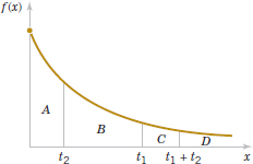
FIGURE 4-24 Lack of memory property of an exponential distribution.
The exponential distribution is often used in reliability studies as the model for the time until failure of a device. For example, the lifetime of a semiconductor chip might be modeled as an exponential random variable with a mean of 40,000 hours. The lack of memory property of the exponential distribution implies that the device does not wear out. That is, regardless of how long the device has been operating, the probability of a failure in the next 1000 hours is the same as the probability of a failure in the first 1000 hours of operation. The lifetime L of a device with failures caused by random shocks might be appropriately modeled as an exponential random variable.
However, the lifetime L of a device that suffers slow mechanical wear, such as bearing wear, is better modeled by a distribution such that P(L < t + Δt|L > t) increases with t. Distributions such as the Weibull distribution are often used in practice to model the failure time of this type of device. The Weibull distribution is presented in a later section.
Exercises FOR SECTION 4-8
![]() Problem available in WileyPLUS at instructor's discretion.
Problem available in WileyPLUS at instructor's discretion.
![]() Go Tutorial Tutoring problem available in WileyPLUS at instructor's discretion.
Go Tutorial Tutoring problem available in WileyPLUS at instructor's discretion.
4-112. ![]() Suppose that X has an exponential distribution with λ = 2. Determine the following:
Suppose that X has an exponential distribution with λ = 2. Determine the following:
(a) P(X ≤ 0)
(b) P(X ≥ 2)
(c) P(X ≤ 1)
(d) P(1 < X < 2)
(e) Find the value of x such that P(X < x) = 0.05.
4-113. ![]() Suppose that X has an exponential distribution with mean equal to 10. Determine the following:
Suppose that X has an exponential distribution with mean equal to 10. Determine the following:
(a) P(X > 10)
(b) P(X > 20)
(c) P(X < 30)
(d) Find the value of x such that P(X < x) = 0.95.
4-114. ![]() Suppose that X has an exponential distribution with a mean of 10. Determine the following:
Suppose that X has an exponential distribution with a mean of 10. Determine the following:
(a) P(X < 5)
(b) P(X < 15|X > 10)
(c) Compare the results in parts (a) and (b) and comment on the role of the lack of memory property.
4-115. ![]() Suppose that the counts recorded by a Geiger counter follow a Poisson process with an average of two counts per minute.
Suppose that the counts recorded by a Geiger counter follow a Poisson process with an average of two counts per minute.
(a) What is the probability that there are no counts in a 30-second interval?
(b) What is the probability that the first count occurs in less than 10 seconds?
(c) What is the probability that the first count occurs between one and two minutes after start-up?
4-116. ![]() Suppose that the log-ons to a computer network follow a Poisson process with an average of three counts per minute.
Suppose that the log-ons to a computer network follow a Poisson process with an average of three counts per minute.
(a) What is the mean time between counts?
(b) What is the standard deviation of the time between counts?
(c) Determine x such that the probability that at least one count occurs before time x minutes is 0.95.
4-117. ![]() The time between calls to a plumbing supply business is exponentially distributed with a mean time between calls of 15 minutes.
The time between calls to a plumbing supply business is exponentially distributed with a mean time between calls of 15 minutes.
(a) What is the probability that there are no calls within a 30-minute interval?
(b) What is the probability that at least one call arrives within a 10-minute interval?
(c) What is the probability that the first call arrives within 5 and 10 minutes after opening?
(d) Determine the length of an interval of time such that the probability of at least one call in the interval is 0.90.
4-118. ![]() The life of automobile voltage regulators has an exponential distribution with a mean life of six years. You purchase a six-year-old automobile, with a working voltage regulator and plan to own it for six years.
The life of automobile voltage regulators has an exponential distribution with a mean life of six years. You purchase a six-year-old automobile, with a working voltage regulator and plan to own it for six years.
(a) What is the probability that the voltage regulator fails during your ownership?
(b) If your regulator fails after you own the automobile three years and it is replaced, what is the mean time until the next failure?
4-119. ![]() Suppose that the time to failure (in hours) of fans in a personal computer can be modeled by an exponential distribution with λ = 0.0003.
Suppose that the time to failure (in hours) of fans in a personal computer can be modeled by an exponential distribution with λ = 0.0003.
(a) What proportion of the fans will last at least 10,000 hours?
(b) What proportion of the fans will last at most 7000 hours?
4-120. ![]() The time between the arrival of electronic messages at your computer is exponentially distributed with a mean of two hours.
The time between the arrival of electronic messages at your computer is exponentially distributed with a mean of two hours.
(a) What is the probability that you do not receive a message during a two-hour period?
(b) If you have not had a message in the last four hours, what is the probability that you do not receive a message in the next two hours?
(c) What is the expected time between your fifth and sixth messages?
4-121. ![]() The time between arrivals of taxis at a busy intersection is exponentially distributed with a mean of 10 minutes.
The time between arrivals of taxis at a busy intersection is exponentially distributed with a mean of 10 minutes.
(a) What is the probability that you wait longer than one hour for a taxi?
(b) Suppose that you have already been waiting for one hour for a taxi. What is the probability that one arrives within the next 10 minutes?
(c) Determine x such that the probability that you wait more than x minutes is 0.10.
(d) Determine x such that the probability that you wait less than x minutes is 0.90.
(e) Determine x such that the probability that you wait less than x minutes is 0.50.
4-122. The number of stork sightings on a route in South Carolina follows a Poisson process with a mean of 2.3 per year.
(a) What is the mean time between sightings?
(b) What is the probability that there are no sightings within three months (0.25 years)?
(c) What is the probability that the time until the first sighting exceeds six months?
(d) What is the probability of no sighting within three years?
4-123. According to results from the analysis of chocolate bars in Chapter 3, the mean number of insect fragments was 14.4 in 225 grams. Assume that the number of fragments follows a Poisson distribution.
(a) What is the mean number of grams of chocolate until a fragment is detected?
(b) What is the probability that there are no fragments in a 28.35-gram (one-ounce) chocolate bar?
(c) Suppose you consume seven one-ounce (28.35-gram) bars this week. What is the probability of no insect fragments?
4-124. ![]() The distance between major cracks in a highway follows an exponential distribution with a mean of five miles.
The distance between major cracks in a highway follows an exponential distribution with a mean of five miles.
(a) What is the probability that there are no major cracks in a 10-mile stretch of the highway?
(b) What is the probability that there are two major cracks in a 10-mile stretch of the highway?
(c) What is the standard deviation of the distance between major cracks?
(d) What is the probability that the first major crack occurs between 12 and 15 miles of the start of inspection?
(e) What is the probability that there are no major cracks in two separate five-mile stretches of the highway?
(f) Given that there are no cracks in the first five miles inspected, what is the probability that there are no major cracks in the next 10 miles inspected?
4-125. ![]() The lifetime of a mechanical assembly in a vibration test is exponentially distributed with a mean of 400 hours.
The lifetime of a mechanical assembly in a vibration test is exponentially distributed with a mean of 400 hours.
(a) What is the probability that an assembly on test fails in less than 100 hours?
(b) What is the probability that an assembly operates for more than 500 hours before failure?
(c) If an assembly has been on test for 400 hours without a failure, what is the probability of a failure in the next 100 hours?
(d) If 10 assemblies are tested, what is the probability that at least one fails in less than 100 hours? Assume that the assemblies fail independently.
(e) If 10 assemblies are tested, what is the probability that all have failed by 800 hours? Assume that the assemblies fail independently.
4-126. ![]() The time between arrivals of small aircraft at a county airport is exponentially distributed with a mean of one hour.
The time between arrivals of small aircraft at a county airport is exponentially distributed with a mean of one hour.
(a) What is the probability that more than three aircraft arrive within an hour?
(b) If 30 separate one-hour intervals are chosen, what is the probability that no interval contains more than three arrivals?
(c) Determine the length of an interval of time (in hours) such that the probability that no arrivals occur during the interval is 0.10.
4-127. The time between calls to a corporate office is exponentially distributed with a mean of 10 minutes.
(a) What is the probability that there are more than three calls in one-half hour?
(b) What is the probability that there are no calls within one-half hour?
(c) Determine x such that the probability that there are no calls within x hours is 0.01.
(d) What is the probability that there are no calls within a two-hour interval?
(e) If four nonoverlapping one-half-hour intervals are selected, what is the probability that none of these intervals contains any call?
(f) Explain the relationship between the results in part (a) and (b).
4-128. ![]() Assume that the flaws along a magnetic tape follow a Poisson distribution with a mean of 0.2 flaw per meter. Let X denote the distance between two successive flaws.
Assume that the flaws along a magnetic tape follow a Poisson distribution with a mean of 0.2 flaw per meter. Let X denote the distance between two successive flaws.
(a) What is the mean of X?
(b) What is the probability that there are no flaws in 10 consecutive meters of tape?
(c) Does your answer to part (b) change if the 10 meters are not consecutive?
(d) How many meters of tape need to be inspected so that the probability that at least one flaw is found is 90%?
(e) What is the probability that the first time the distance between two flaws exceeds eight meters is at the fifth flaw?
(f) What is the mean number of flaws before a distance between two flaws exceeds eight meters?
4-129. If the random variable X has an exponential distribution with mean θ, determine the following:
(a) P(X > θ)
(b) P(X > 2θ)
(c) P(X > 3θ)
(d) How do the results depend on θ?
4-130. ![]() Derive the formula for the mean and variance of an exponential random variable.
Derive the formula for the mean and variance of an exponential random variable.
4-131. Web crawlers need to estimate the frequency of changes to Web sites to maintain a current index for Web searches. Assume that the changes to a Web site follow a Poisson process with a mean of 3.5 days.
(a) What is the probability that the next change occurs in less than 2.0 days?
(b) What is the probability that the time until the next change is greater 7.0 days?
(c) What is the time of the next change that is exceeded with probability 90%?
(d) What is the probability that the next change occurs in less than 10.0 days, given that it has not yet occurred after 3.0 days?
4-132. The length of stay at a specific emergency department in a hospital in Phoenix, Arizona had a mean of 4.6 hours. Assume that the length of stay is exponentially distributed.
(a) What is the standard deviation of the length of stay?
(b) What is the probability of a length of stay of more than 10 hours?
(c) What length of stay is exceeded by 25% of the visits?
4-133. An article in Journal of National Cancer Institute [“Breast Cancer Screening Policies in Developing Countries: A Cost-Effectiveness Analysis for India” (2008, Vol. 100(18), pp. 1290–1300)] presented a screening analysis model of breast cancer based on data from India. In this analysis, the time that a breast cancer case stays in a preclinical state is modeled to be exponentially distributed with a mean depending on the state. For example, the time that a cancer case stays in the state of T1C (tumor size of 11–20 mm) is exponentially distributed with a mean of 1.48 years.
(a) What is the probability that a breast cancer case in India stays in the state of T1C for more than 2.0 years?
(b) What is the proportion of breast cancer cases in India that spend at least 1.0 year in the state of T1C?
(c) Assume that a person in India is diagnosed to be in the state of T1C. What is the probability that the patient is in the same state six months later?
4-134. Requests for service in a queuing model follow a Poisson distribution with a mean of five per unit time.
(a) What is the probability that the time until the first request is less than 4 minutes?
(b) What is the probability that the time between the second and third requests is greater than 7.5 time units?
(c) Determine the mean rate of requests such that the probability is 0.9 that there are no requests in 0.5 time units.
(d) If the service times are independent and exponentially distributed with a mean of 0.4 time units, what can you conclude about the long-term response of this system to requests?
4-135. An article in Vaccine [“Modeling the Effects of Influenza Vaccination of Health Care Workers in Hospital Departments” (2009, Vol. 27(44), pp. 6261–6267)] considered the immunization of healthcare workers to reduce the hazard rate of influenza virus infection for patients in regular hospital departments. In this analysis, each patient's length of stay in the department is taken as exponentially distributed with a mean of 7.0 days.
(a) What is the probability that a patient stays in hospital for less than 5.5 days?
(b) What is the probability that a patient stays in hospital for more than 10.0 days if the patient has currently stayed for 7.0 days?
(c) Determine the mean length of stay such that the probability is 0.9 that a patient stays in the hospital less than 6.0 days.
4-136. An article in Ad Hoc Networks [“Underwater Acoustic Sensor Networks: Target Size Detection and Performance Analysis” (2009, Vol. 7(4), pp. 803–808)] discussed an underwater acoustic sensor network to monitor a given area in an ocean. The network does not use cables and does not interfere with shipping activities. The arrival of clusters of signals generated by the same pulse is taken as a Poisson arrival process with a mean of λ per unit time. Suppose that for a specific underwater acoustic sensor network, this Poisson process has a rate of 2.5 arrivals per unit time.
(a) What is the mean time between 2.0 consecutive arrivals?
(b) What is the probability that there are no arrivals within 0.3 time units?
(c) What is the probability that the time until the first arrival exceeds 1.0 unit of time?
(d) Determine the mean arrival rate such that the probability is 0.9 that there are no arrivals in 0.3 time units.
4-9 Erlang and Gamma Distributions
An exponential random variable describes the length until the first count is obtained in a Poisson process. A generalization of the exponential distribution is the length until r events occur in a Poisson process. Consider Example 4-23.
Example 4-23 Processor Failure The failures of the central processor units of large computer systems are often modeled as a Poisson process. Typically, failures are not caused by components wearing out but by more random failures of the large number of semiconductor circuits in the units. Assume that the units that fail are immediately repaired, and assume that the mean number of failures per hour is 0.0001. Let X denote the time until four failures occur in a system. Determine the probability that X exceeds 40,000 hours.
Let the random variable N denote the number of failures in 40,000 hours of operation. The time until four failures occur exceeds 40,000 hours if and only if the number of failures in 40,000 hours is three or less. Therefore,
![]()
The assumption that the failures follow a Poisson process implies that N has a Poisson distribution with
![]()
Therefore,
![]()
The previous example can be generalized to show that if X is the time until the rth event in a Poisson process, then
![]()
Because P(X > x) = 1 − F(x), the probability density function of X equals the negative of the derivative of the right-hand side of the previous equation. After extensive algebraic simplification, the probability density function of X can be shown to equal
![]()
This probability density function defines an Erlang random variable. Clearly, an Erlang random variable with r = 1 is an exponential random variable.
It is convenient to generalize the Erlang distribution to allow r to assume any non-negative value. Then the Erlang and some other common distributions become special cases of this generalized distribution. To accomplish this step, the factorial function (r − 1)! is generalized to apply to any non-negative value of r, but the generalized function should still equal (r − 1)! when r is a positive integer.
Gamma Function
The gamma function is
![]()
It can be shown that the integral in the definition of Γ(r) is finite. Furthermore, by using integration by parts, it can be shown that
![]()
This result is left as an exercise. Therefore, if r is a positive integer (as in the Erlang distribution),
![]()
Also, Γ(1) = 0! = 1 and it can be shown that Γ(1/2) = π1/2. The gamma function can be interpreted as a generalization to noninteger values of r of the term that is used in the Erlang probability density function. Now the Erlang distribution can be generalized.
Gamma Distribution
The random variable X with probability density function

is a gamma random variable with parameters λ > 0 and r > 0. If r is an integer, X has an Erlang distribution.
The parameters λ and r are often called the scale and shape parameters, respectively. However, one should check the definitions used in software packages. For example, some statistical software defines the scale parameter as 1/λ. Sketches of the gamma distribution for several values of λ and r are shown in Fig. 4-25. Many different shapes can be generated from changes to the parameters. Also, the change of variable u = λx and the definition of the gamma function can be used to show that the probability density function integrates to 1.
For the special case when r is an integer and the value of r is not large, Equation (4-17) can be applied to calculate probabilities for a gamma random variable. However, in general, the integral of the gamma probability density function is difficult to evaluate so computer software is used to determine probabilities.
Recall that for an exponential distribution with parameter λ, the mean and variance are 1/λ and 1/λ2, respectively. An Erlang random variable is the time until the rth event in a Poisson process and the time between events are independent. Therefore, it is plausible that the mean and variance of a gamma random variable multiply the exponential results by r. This motivates the following conclusions. Repeated integration by parts can be used to derive these, but the details are lengthy and omitted.
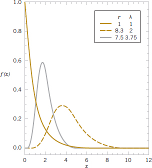
FIGURE 4-25 Gamma probability density functions for selected values of λ and r.
Mean and Variance
If X is a gamma random variable with parameters λ and r,
![]()
Example 4-24 The time to prepare a micro-array slide for high-throughput genomics is a Poisson process with a mean of two hours per slide. What is the probability that 10 slides require more than 25 hours to prepare?
Let X denote the time to prepare 10 slides. Because of the assumption of a Poisson process, X has a gamma distribution with λ = 1/2, r = 10, and the requested probability is P(X > 25). The probability can be obtained from software that provides cumulative Poisson probabilities or gamma probabilities. For the cumulative Poisson probabilities, we use the method in Example 4-23 to obtain
![]()
In software we set the mean = 12.5 and the input = 9 to obtain P(X > 25) = 0.2014.
As a check, we use the gamma cumulative probability function in Minitab. Set the shape parameter to 10, the scale parameter to 0.5, and the input to 25. The probability computed is P(X ≤ 25) = 0.7986, and when this is subtracted from one we match with the previous result that P(X > 25) = 0.2014.
What are the mean and standard deviation of the time to prepare 10 slides? The mean time is
![]()
The variance of time is
![]()
so that the standard deviation is 401/2 = 6.32 hours.
The slides will be completed by what length of time with probability equal to 0.95? The question asks for x such that
![]()
where X is gamma with λ = 0.5 and r = 10. In software, we use the gamma inverse cumulative probability function and set the shape parameter to 10, the scale parameter to 0.5, and the probability to 0.95. The solution is
![]()
Practical Interpretation: Based on this result, a schedule that allows 31.41 hours to prepare 10 slides should be met 95% of the time.
Furthermore, the chi-squared distribution is a special case of the gamma distribution in which λ = 1/2 and r equals one of the values 1/2,1, 3/2, 2, .... This distribution is used extensively in interval estimation and tests of hypotheses that are discussed in subsequent chapters. The chi-squared distribution is discussed in Chapter 7.
EXERCISES FOR SECTION 4-9
![]() Problem available in WileyPLUS at instructor's discretion.
Problem available in WileyPLUS at instructor's discretion.
![]() Go Tutorial Tutoring problem available in WileyPLUS at instructor's discretion.
Go Tutorial Tutoring problem available in WileyPLUS at instructor's discretion.
4-137. ![]() Use the properties of the gamma function to evaluate the following:
Use the properties of the gamma function to evaluate the following:
(a) Γ(6)
(b) Γ(5/2)
(c) Γ(9/2)
4-138. ![]() Given the probability density function f(x) = 0.013x2e−0.01x /Γ(3), determine the mean and variance of the distribution.
Given the probability density function f(x) = 0.013x2e−0.01x /Γ(3), determine the mean and variance of the distribution.
4-139. ![]() Calls to a telephone system follow a Poisson distribution with a mean of five calls per minute.
Calls to a telephone system follow a Poisson distribution with a mean of five calls per minute.
(a) What is the name applied to the distribution and parameter values of the time until the 10th call?
(b) What is the mean time until the 10th call?
(c) What is the mean time between the 9th and 10th calls?
(d) What is the probability that exactly four calls occur within one minute?
(e) If 10 separate one-minute intervals are chosen, what is the probability that all intervals contain more than two calls?
4-140. ![]() Raw materials are studied for contamination. Suppose that the number of particles of contamination per pound of material is a Poisson random variable with a mean of 0.01 particle per pound.
Raw materials are studied for contamination. Suppose that the number of particles of contamination per pound of material is a Poisson random variable with a mean of 0.01 particle per pound.
(a) What is the expected number of pounds of material required to obtain 15 particles of contamination?
(b) What is the standard deviation of the pounds of materials required to obtain 15 particles of contamination?
4-141. ![]() The time between failures of a laser in a cytogenics machine is exponentially distributed with a mean of 25,000 hours.
The time between failures of a laser in a cytogenics machine is exponentially distributed with a mean of 25,000 hours.
(a) What is the expected time until the second failure?
(b) What is the probability that the time until the third failure exceeds 50,000 hours?
4-142. ![]() In a data communication system, several messages that arrive at a node are bundled into a packet before they are transmitted over the network. Assume that the messages arrive at the node according to a Poisson process with τ = 30 messages per minute. Five messages are used to form a packet.
In a data communication system, several messages that arrive at a node are bundled into a packet before they are transmitted over the network. Assume that the messages arrive at the node according to a Poisson process with τ = 30 messages per minute. Five messages are used to form a packet.
(a) What is the mean time until a packet is formed, that is, until five messages have arrived at the node?
(b) What is the standard deviation of the time until a packet is formed?
(c) What is the probability that a packet is formed in less than 10 seconds?
(d) What is the probability that a packet is formed in less than five seconds?
4-143. ![]() Errors caused by contamination on optical disks occur at the rate of one error every 105 bits. Assume that the errors follow a Poisson distribution.
Errors caused by contamination on optical disks occur at the rate of one error every 105 bits. Assume that the errors follow a Poisson distribution.
(a) What is the mean number of bits until five errors occur?
(b) What is the standard deviation of the number of bits until five errors occur?
(c) The error-correcting code might be ineffective if there are three or more errors within 105 bits. What is the probability of this event?
4-144. ![]() Calls to the help line of a large computer distributor follow a Poisson distribution with a mean of 20 calls per minute. Determine the following:
Calls to the help line of a large computer distributor follow a Poisson distribution with a mean of 20 calls per minute. Determine the following:
(a) Mean time until the one-hundredth call
(b) Mean time between call numbers 50 and 80
(c) Probability that three or more calls occur within 15 seconds
4-145. ![]() The time between arrivals of customers at an automatic teller machine is an exponential random variable with a mean of five minutes.
The time between arrivals of customers at an automatic teller machine is an exponential random variable with a mean of five minutes.
(a) What is the probability that more than three customers arrive in 10 minutes?
(b) What is the probability that the time until the fifth customer arrives is less than 15 minutes?
4-146. Use integration by parts to show that Γ(r) = (r − 1)Γ(r − 1).
4-147. Show that the gamma density function f(x, λ, r) integrates to 1.
4-148. ![]() Use the result for the gamma distribution to determine the mean and variance of a chi-square distribution with r = 7/2.
Use the result for the gamma distribution to determine the mean and variance of a chi-square distribution with r = 7/2.
4-149. Patients arrive at a hospital emergency department according to a Poisson process with a mean of 6.5 per hour.
(a) What is the mean time until the 10th arrival?
(b) What is the probability that more than 20 minutes is required for the third arrival?
4-150. The total service time of a multistep manufacturing operation has a gamma distribution with mean 18 minutes and standard deviation 6.
(a) Determine the parameters λ and r of the distribution.
(b) Assume that each step has the same distribution for service time. What distribution for each step and how many steps produce this gamma distribution of total service time?
4-51. An article in Sensors and Actuators A: Physical [“Characterization and Simulation of Avalanche PhotoDiodes for Next-Generation Colliders” (2011, Vol. 172(1), pp. 181–188)] considered an avalanche photodiode (APD) to detect charged particles in a photo. The number of arrivals in each detection window was modeled with a Poisson distribution with a mean depending on the intensity of beam. For one beam intensity, the number of electrons arriving at an APD follows a Poisson distribution with a mean of 1.74 particles per detection window of 200 nanoseconds.
(a) What is the mean and variance of the time for 100 arrivals?
(b) What is the probability that the time until the fifth particle arrives is greater than 1.0 nanosecond?
4-52. An article in Mathematical Biosciences [“Influence of Delayed Viral Production on Viral Dynamics in HIV-1 Infected Patients” (1998, Vol. 152(2), pp. 143–163)] considered the time delay between the initial infection by immunodeficiency virus type 1 (HIV-1) and the formation of productively infected cells. In the simulation model, the time delay is approximated by a gamma distribution with parameters r = 4 and 1/λ = 0.25 days. Determine the following:
(a) Mean and variance of time delay
(b) Probability that a time delay is more than half a day
(c) Probability that a time delay is between one-half and one day
4-10 Weibull Distribution
As mentioned previously, the Weibull distribution is often used to model the time until failure of many different physical systems. The parameters in the distribution provide a great deal of flexibility to model systems in which the number of failures increases with time (bearing wear), decreases with time (some semiconductors), or remains constant with time (failures caused by external shocks to the system).
Weibull Distribution
The random variable X with probability density function
![]()
is a Weibull random variable with scale parameter δ > 0 and shape parameter β > 0.
The graphs of selected probability density functions in Fig. 4-26 illustrate the flexibility of the Weibull distribution. By inspecting the probability density function, we can see that when β = 1, the Weibull distribution is identical to the exponential distribution. Also, the Raleigh distribution is a special case when the shape parameter is 2.
The cumulative distribution function is often used to compute probabilities. The following result can be obtained.
Cumulative Distribution Function
If X has a Weibull distribution with parameters δ and β, then the cumulative distribution function of X is
![]()
Also, the following results can be obtained.
Mean and Variance
If X has a Weibull distribution with parameters δ and β,
![]()

FIGURE 4-26 Weibull probability density functions for selected values of δ and β.
Example 4-25 Bearing Wear The time to failure (in hours) of a bearing in a mechanical shaft is satisfactorily modeled as a Weibull random variable with β = 1/2 and δ = 5000 hours. Determine the mean time until failure.
From the expression for the mean,
![]()
Determine the probability that a bearing lasts at least 6000 hours. Now,
![]()
Practical Interpretation: Consequently, only 23.7% of all bearings last at least 6000 hours.
EXERCISES FOR SECTION 4-10
![]() Problem available in WileyPLUS at instructor's discretion.
Problem available in WileyPLUS at instructor's discretion.
![]() Go Tutorial Tutoring problem available in WileyPLUS at instructor's discretion.
Go Tutorial Tutoring problem available in WileyPLUS at instructor's discretion.
4-153. ![]() Suppose that X has a Weibull distribution with β = 0.2 and δ = 100 hours. Determine the mean and variance of X.
Suppose that X has a Weibull distribution with β = 0.2 and δ = 100 hours. Determine the mean and variance of X.
4-154. ![]() Suppose that X has a Weibull distribution with β = 0.2 and δ = 100 hours. Determine the following:
Suppose that X has a Weibull distribution with β = 0.2 and δ = 100 hours. Determine the following:
(a) P(X < 10,000)
(b) P(X > 5000)
4-155. ![]() If X is a Weibull random variable with β = 1 and δ = 1000, what is another name for the distribution of X, and what is the mean of X?
If X is a Weibull random variable with β = 1 and δ = 1000, what is another name for the distribution of X, and what is the mean of X?
4-156. ![]() Assume that the life of a roller bearing follows a Weibull distribution with parameters β = 2 and δ = 10,000 hours.
Assume that the life of a roller bearing follows a Weibull distribution with parameters β = 2 and δ = 10,000 hours.
(a) Determine the probability that a bearing lasts at least 8000 hours.
(b) Determine the mean time until failure of a bearing.
(c) If 10 bearings are in use and failures occur independently, what is the probability that all 10 bearings last at least 8000 hours?
4-157. ![]() The life (in hours) of a computer processing unit (CPU) is modeled by a Weibull distribution with parameters β = 3 and δ = 900 hours. Determine (a) and (b):
The life (in hours) of a computer processing unit (CPU) is modeled by a Weibull distribution with parameters β = 3 and δ = 900 hours. Determine (a) and (b):
(a) Mean life of the CPU.
(b) Variance of the life of the CPU.
(c) What is the probability that the CPU fails before 500 hours?
4-158. ![]() Assume that the life of a packaged magnetic disk exposed to corrosive gases has a Weibull distribution with β = 0.5 and the mean life is 600 hours. Determine the following:
Assume that the life of a packaged magnetic disk exposed to corrosive gases has a Weibull distribution with β = 0.5 and the mean life is 600 hours. Determine the following:
(a) Probability that a disk lasts at least 500 hours.
(b) Probability that a disk fails before 400 hours.
4-159. ![]() The life (in hours) of a magnetic resonance imaging machine (MRI) is modeled by a Weibull distribution with parameters β = 2 and δ = 500 hours. Determine the following:
The life (in hours) of a magnetic resonance imaging machine (MRI) is modeled by a Weibull distribution with parameters β = 2 and δ = 500 hours. Determine the following:
(a) Mean life of the MRI
(b) Variance of the life of the MRI
(c) Probability that the MRI fails before 250 hours.
4-160. ![]() An article in the Journal of the Indian Geophysical Union titled “Weibull and Gamma Distributions for Wave Parameter Predictions” (2005, Vol. 9, pp. 55–64) described the use of the Weibull distribution to model ocean wave heights. Assume that the mean wave height at the observation station is 2.5 m and the shape parameter equals 2. Determine the standard deviation of wave height.
An article in the Journal of the Indian Geophysical Union titled “Weibull and Gamma Distributions for Wave Parameter Predictions” (2005, Vol. 9, pp. 55–64) described the use of the Weibull distribution to model ocean wave heights. Assume that the mean wave height at the observation station is 2.5 m and the shape parameter equals 2. Determine the standard deviation of wave height.
4-161. An article in the Journal of Geophysical Research [“Spatial and Temporal Distributions of U.S. of Winds and Wind Power at 80 m Derived from Measurements” (2003, vol. 108)] considered wind speed at stations throughout the United States. A Weibull distribution can be used to model the distribution of wind speeds at a given location. Every location is characterized by a particular shape and scale parameter. For a station at Amarillo, Texas, the mean wind speed at 80 m (the hub height of large wind turbines) in 2000 was 10.3 m/s with a standard deviation of 4.9 m/s. Determine the shape and scale parameters of a Weibull distribution with these properties.
4-162. Suppose that X has a Weibull distribution with β = 2 and δ = 8.6. Determine the following:
(a) P(X < 10)
(b) P(X > 9)
(c) P(8 < X < 11)
(d) Value for x such that P(X > x) = 0.9
4-163. Suppose that the lifetime of a component (in hours) is modeled with a Weibull distribution with β = 2 and δ = 4000. Determine the following in parts (a) and (b):
(a) P(X > 3000)
(b) P(X > 6000|X > 3000)
(c) Comment on the probabilities in the previous parts compared to the results for an exponential distribution.
4-164. Suppose that the lifetime of a component (in hours), X is modeled with a Weibull distribution with β = 0.5 and δ = 4000.
Determine the following in parts (a) and (b):
(a) P(X > 3500)
(b) P(X > 6000|X > 3000)
(c) Comment on the probabilities in the previous parts compared to the results for an exponential distribution.
(d) Comment on the role of the parameter β in a lifetime model with the Weibull distribution.
4-165. Suppose that X has a Weibull distribution with β = 2 and δ = 2000. Determine the following in parts (a) and (b):
(a) P(X > 3500)
(b) P(X > 3500) for an exponential random variable with the same mean as the Weibull distribution
(c) Comment on the probability that the lifetime exceeds 3500 hours under the Weibull and exponential distributions.
4-166. An article in Electronic Journal of Applied Statistical Analysis [“Survival Analysis of Dialysis Patients Under Parametric and Non-Parametric Approaches” (2012, Vol. 5(2), pp. 271–288)] modeled the survival time of dialysis patients with chronic kidney disease with a Weibull distribution. The mean and standard deviation of survival time were 16.01 and 11.66 months, respectively. Determine the following:
(a) Shape and scale parameters of this Weibull distribution
(b) Probability that survival time is more than 48 months
(c) Survival time exceeded with 90% probability
4-167. An article in Proceeding of the 33rd International ACM SIGIR Conference on Research and Development in Information Retrieval [“Understanding Web Browsing Behaviors Through Weibull Analysis of Dwell Time” (2010, p. 379l–386)] proposed that a Weibull distribution can be used to model Web page dwell time (the length of time a Web visitor spends on a Web page). For a specific Web page, the shape and scale parameters are 1 and 300 seconds, respectively. Determine the following:
(a) Mean and variance of dwell time
(b) Probability that a Web user spends more than four minutes on this Web page
(c) Dwell time exceeded with probability 0.25
4-168. An article in Financial Markets Institutions and Instruments [“Pricing Reinsurance Contracts on FDIC Losses” (2008, Vol. 17(3)] modeled average annual losses (in billions of dollars) of the Federal Deposit Insurance Corporation (FDIC) with a Weibull distribution with parameters δ = 1.9317 and β = 0.8472. Determine the following:
(a) Probability of a loss greater than $2 billion
(b) Probability of a loss between $2 and $4 billion
(c) Value exceeded with probability 0.05
(d) Mean and standard deviation of loss
4-169. An article in IEEE Transactions on Dielectrics and Electrical Insulation [“Statistical Analysis of the AC Breakdown Voltages of Ester Based Transformer Oils” (2008, Vol. 15(4))] used Weibull distributions to model the breakdown voltage of insulators. The breakdown voltage is the minimum voltage at which the insulator conducts. For 1 mm of natural ester, the 1% probability of breakdown voltage is approximately 26 kV, and the 7% probability is approximately 31.6 kV. Determine the parameters δ and β of the Weibull distribution.
4-11 Lognormal Distribution
Variables in a system sometimes follow an exponential relationship as x = exp(w). If the exponent is a random variable W, then X = exp(W) is a random variable with a distribution of interest. An important special case occurs when W has a normal distribution. In that case, the distribution of X is called a lognormal distribution. The name follows from the transformation ln (X) = W. That is, the natural logarithm of X is normally distributed.
Probabilities for X are obtained from the transform of the normal distribution. The range of X is (0, ∞). Suppose that W is normally distributed with mean θ and variance ω2; then the cumulative distribution function for X is

for x > 0, where Z is a standard normal random variable and Φ(·) is the cumulative distribution function of the standard normal distribution. Therefore, Appendix Table III can be used to determine the probability. Also, F(x) = 0 for x ≤ 0.
The probability density function of X can be obtained from the derivative of F(x). This derivative is applied to the last term in the expression for F(x). Because Φ(·) is the integral of the standard normal density function, the fundamental theorem of calculus is used to calculate the derivative. Furthermore, from the probability density function, the mean and variance of X can be derived. The details are omitted, but a summary of results follows.
Lognormal Distribution
Let W have a normal distribution with mean θ and variance ω2; then X = exp(W) is a lognormal random variable with probability density function
![]()
The mean and variance of X are
![]()
The parameters of a lognormal distribution are θ and ω2, but these are the mean and variance of the normal random variable W. The mean and variance of X are the functions of these parameters shown in Equation (4-22). Figure 4-27 illustrates lognormal distributions for selected values of the parameters.
The lifetime of a product that degrades over time is often modeled by a lognormal random variable. For example, this is a common distribution for the lifetime of a semiconductor laser. A Weibull distribution can also be used in this type of application, and with an appropriate choice for parameters, it can approximate a selected lognormal distribution. However, a lognormal distribution is derived from a simple exponential function of a normal random variable, so it is easy to understand and easy to evaluate probabilities.

FIGURE 4-27 Lognormal probability density functions with θ = 0 for selected values of ω2.
Example 4-26 Semiconductor Laser The lifetime (in hours) of a semiconductor laser has a lognormal distribution with θ = 10 and ω = 1.5. What is the probability that the lifetime exceeds 10,000 hours?
From the cumulative distribution function for X,

What lifetime is exceeded by 99% of lasers? The question is to determine x such that P(X > x) = 0.99. Therefore,
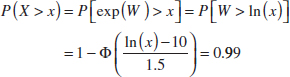
From Appendix Table III, 1 − Φ(z) = 0.99 when z = −2.33. Therefore,
![]()
Determine the mean and standard deviation of lifetime. Now

so the standard deviation of X is 197,661.5 hours.
Practical Interpretation: The standard deviation of a lognormal random variable can be large relative to the mean.
Exercises FOR SECTION 4-11
![]() Problem available in WileyPLUS at instructor's discretion.
Problem available in WileyPLUS at instructor's discretion.
![]() Go Tutorial Tutoring problem available in WileyPLUS at instructor's discretion.
Go Tutorial Tutoring problem available in WileyPLUS at instructor's discretion.
4-170. ![]() Suppose that X has a lognormal distribution with parameters θ = 5 and ω2 = 9. Determine the following:
Suppose that X has a lognormal distribution with parameters θ = 5 and ω2 = 9. Determine the following:
(a) P(X < 13,300)
(b) Value for x such that P(X ≤ x) = 0.95
(c) Mean and variance of X
4-171. ![]() Suppose that X has a lognormal distribution with parameters θ = −2 and ω2 = 9. Determine the following:
Suppose that X has a lognormal distribution with parameters θ = −2 and ω2 = 9. Determine the following:
(a) P(500 < X < 1000)
(b) Value for x such that P(X < x) = 0.1
(c) Mean and variance of X
4-172. ![]() Suppose that X has a lognormal distribution with parameters θ = 2 and ω2 = 4. Determine the following in parts (a) and (b):
Suppose that X has a lognormal distribution with parameters θ = 2 and ω2 = 4. Determine the following in parts (a) and (b):
(a) P(X < 500)
(b) Conditional probability that X < 1500 given that X > 1000
(c) What does the difference between the probabilities in parts (a) and (b) imply about lifetimes of lognormal random variables?
4-173. ![]() The length of time (in seconds) that a user views a page on a Web site before moving to another page is a lognormal random variable with parameters θ = 0.5 and ω2 = 1.
The length of time (in seconds) that a user views a page on a Web site before moving to another page is a lognormal random variable with parameters θ = 0.5 and ω2 = 1.
(a) What is the probability that a page is viewed for more than 10 seconds?
(b) By what length of time have 50% of the users moved to another page?
(c) What are the mean and standard deviation of the time until a user moves from the page?
4-174. ![]() Suppose that X has a lognormal distribution and that the mean and variance of X are 100 and 85,000, respectively. Determine the parameters θ and ω2 of the lognormal distribution. [Hint: define x = exp(θ) and y = exp(ω2) and write two equations in terms of x and y.]
Suppose that X has a lognormal distribution and that the mean and variance of X are 100 and 85,000, respectively. Determine the parameters θ and ω2 of the lognormal distribution. [Hint: define x = exp(θ) and y = exp(ω2) and write two equations in terms of x and y.]
4-175. ![]() The lifetime of a semiconductor laser has a lognormal distribution, and it is known that the mean and standard deviation of lifetime are 10,000 and 20,000, respectively.
The lifetime of a semiconductor laser has a lognormal distribution, and it is known that the mean and standard deviation of lifetime are 10,000 and 20,000, respectively.
(a) Calculate the parameters of the lognormal distribution.
(b) Determine the probability that a lifetime exceeds 10,000 hours.
(c) Determine the lifetime that is exceeded by 90% of lasers.
4-176. ![]() An article in Health and Population: Perspectives and Issues (2000, Vol. 23, pp. 28–36) used the lognormal distribution to model blood pressure in humans. The mean systolic blood pressure (SBP) in males age 17 was 120.87 mm Hg. If the co-efficient of variation (100% × Standard deviation/mean) is 9%, what are the parameter values of the lognormal distribution?
An article in Health and Population: Perspectives and Issues (2000, Vol. 23, pp. 28–36) used the lognormal distribution to model blood pressure in humans. The mean systolic blood pressure (SBP) in males age 17 was 120.87 mm Hg. If the co-efficient of variation (100% × Standard deviation/mean) is 9%, what are the parameter values of the lognormal distribution?
4-177. Derive the probability density function of a lognormal random variable from the derivative of the cumulative distribution function.
4-178. Suppose that X has a lognormal distribution with parameters θ = 10 and ω2 = 16. Determine the following:
(a) P(X < 2000)
(b) P(X > 1500)
(c) Value exceeded with probability 0.7
4-179. Suppose that the length of stay (in hours) at a hospital emergency department is modeled with a lognormal random variable X with θ = 1.5 and ω = 0.4. Determine the following in parts (a) and (b):
(a) Mean and variance
(b) P(X < 8)
(c) Comment on the difference between the probability P(X < 0) calculated from this lognormal distribution and a normal distribution with the same mean and variance.
4-180. An article in Journal of Hydrology [“Use of a Lognormal Distribution Model for Estimating Soil Water Retention Curves from Particle-Size Distribution Data” (2006, Vol. 323(1), pp. 325–334)] considered a lognormal distribution model to estimate water retention curves for a range of soil textures. The particle-size distribution (in centimeters) was modeled as a lognormal random variable X with θ = −3.8 and ω = 0.7. Determine the following:
(a) P(X < 0.02)
(b) Value for x such that P(X ≤ x) = 0.95.
(c) Mean and variance of X
4-181. An article in Applied Mathematics and Computation [“Confidence Intervals for Steady State Availability of a System with Exponential Operating Time and Lognormal Repair Time” (2003, Vol. 137(2), pp. 499-509)] considered the long-run availability of a system with an assumed lognormal distribution for repair time. In a given example, repair time follows a lognormal distribution with θ = ω = 1. Determine the following:
(a) Probability that repair time is more than five time units
(b) Conditional probability that a repair time is less than eight time units given that it is more than five time units
(c) Mean and variance of repair time
4-182. An article in Chemosphere [“Statistical Evaluations Reflecting the Skewness in the Distribution of TCDD Levels in Human Adipose Tissue” (1987, Vol. 16(8), pp. 2135-2140)] concluded that the levels of 2,3,7,8-TCDD (colorless persistent environmental contaminants with no distinguishable odor at room temperature) in human adipose tissue has a lognormal distribution (based on empirical evidence from North America). The mean and variance of this lognormal distribution in the USA are 8 and 21, respectively. Let X denote this lognormal random variable. Determine the following:
(a) P(2000 < X < 2500)
(b) Value exceeded with probability 10%
(c) Mean and variance of X
4-183. Consider the lifetime of a laser in Example 4-26. Determine the following in parts (a) and (b):
(a) Probability the lifetime is less than 1000 hours
(b) Probability the lifetime is less than 11,000 hours given that it is more than 10,000 hours
(c) Compare the answers to parts (a) and (b) and comment on any differences between the lognormal and exponential distributions.
4-12 Beta Distribution
A continuous distribution that is flexble but bounded over a finite range is useful for probability models. The proportion of solar radiation absorbed by a material or the proportion (of the maximum time) required to complete a task in a project are examples of continuous random variables over the interval [0, 1].
The random variable X with probability density function
![]()
is a beta random variable with parameters α > 0 and β > 0.
The shape parameters α and β allow the probability density function to assume many different shapes. Figure 4-28 provides some examples. If α = β, the distribution is symmetric about x = 0.5, and if α = β = 1, the beta distribution equals a continuous uniform distribution. Figure 4-28 illustrates that other parameter choices generate nonsymmetric distributions.
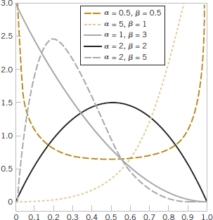
FIGURE 4-28 Beta probability density functions for selected values of the parameters α and β.
In general, there is a not a closed-form expression for the cumulative distribution function, and probabilities for beta random variables need to be computed numerically. The exercises provide some special cases in which the probability density function is more easily handled.
Example 4-27 Consider the completion time of a large commercial development. The proportion of the maximum allowed time to complete a task is modeled as a beta random variable with α = 2.5 and β = 1. What is the probability that the proportion of the maximum time exceeds 0.7?
Suppose that X denotes the proportion of the maximum time required to complete the task. The probability is

If α > 1 and β > 1, the mode (peak of the density) is in the interior of [0, 1] and equals
![]()
This expression is useful to relate the peak of the density to the parameters. Suppose that the proportion of time to complete one task among several follows a beta distribution with α = 2.5 and β = 1. The mode of this distribution is (2.5 − 1)/(3.5 − 2) = 1. The mean and variance of a beta distribution can be obtained from the integrals, but the details are left to a Mind-Expanding exercise.
Also, although a beta random variable X is defined over the interval [0, 1], a random variable W defined over the finite interval [a, b] can be constructed from W = a + (b − a)X.
Mean and Variance
If X has a beta distribution with parameters α and β,
![]()
Example 4-28 The time to complete a task in a large project is modeled as a generalized beta distribution with minimum and maximum times a = 8 and b = 20 days, respectively, along with mode of m = 16 days. Also, assume that the mean completion time is μ = (a + 4m + b)/6. Determine the parameters α and β of the generalized beta distribution with these properties.
The values (a, m, b) specify the minimum, mode, and maximum times, but the mode value alone does not uniquely determine the two parameters α and β. Consequently, the mean completion time, μ, is assumed to equal μ = (a + 4m + b)/6.
Here the generalized beta random variable is W = a + (b − a)X, where X is a beta random variable. Because the minimum and maximum values for W are 8 and 20, respectively, a = 8 and b = 20. The mean of W is
![]()
The assumed mean is μ = (8 + 4(16) + 20)/6 = 15.333. The mode of W is
![]()
with m = 16. These equations can be solved for α and β to obtain

Therefore,

Practical Interpretation: The program evaluation and review technique (PERT) widely uses the distribution of W to model the duration of tasks. Therefore, W is said to have a PERT distribution. Notice that we need only specify the minimum, maximum, and mode (most likely time) for a task to specify the distribution. The model assumes that the mean is the function of these three values and allows the α and β parameters to be computed.
Exercises FOR SECTION 4-12
![]() Problem available in WileyPLUS at instructor's discretion.
Problem available in WileyPLUS at instructor's discretion.
![]() Go Tutorial Tutoring problem available in WileyPLUS at instructor's discretion.
Go Tutorial Tutoring problem available in WileyPLUS at instructor's discretion.
4-184. Suppose that x has a beta distribution with parameters α = 2.5 and β = 2.5. Sketch an approximate graph of the probability density function. Is the density symmetric?
4-185. Suppose that x has a beta distribution with parameters α = 2.5 and β = 1. Determine the following:
(a) P(X < 0.25)
(b) P(0.25 < X < 0.75)
(c) Mean and variance
4-186. Suppose that X has a beta distribution with parameters α = 1 and β = 4.2. Determine the following:
(a) P(X < 0.25)
(b) P(0.5 < X)
(c) Mean and variance
4-187. A European standard value for a low-emission window glazing uses 0.59 as the proportion of solar energy that enters a room. Suppose that the distribution of the proportion of solar energy that enters a room is a beta random variable.
(a) Calculate the mode, mean, and variance of the distribution for α = 3 and β = 1.4.
(b) Calculate the mode, mean, and variance of the distribution for α = 10 and β = 6.25.
(c) Comment on the difference in dispersion in the distribution from parts (a) and (b).
4-188. The length of stay at a hospital emergency department is the sum of the waiting and service times. Let X denote the proportion of time spent waiting and assume a beta distribution with α = 10 and β = 1. Determine the following:
(a) P(X > 0.9)
(b) P(X < 0.5)
(c) Mean and variance
4-189. The maximum time to complete a task in a project is 2.5 days. Suppose that the completion time as a proportion of this maximum is a beta random variable with α = 2 and β = 3. What is the probability that the task requires more than two days to complete?
4-190. An allele is an alternate form of a gene, and the proportion of alleles in a population is of interest in genetics. An article in BMC Genetics [“Calculating Expected DNA Remnants From Ancient Founding Events in Human Population Genetics” (2008, Vol. 9:66)] used a beta distribution with mean 0.3 and standard deviation 0.17 to model initial allele proportions in a genetic simulation. Determine the parameters α and β for this beta distribution.
4-191. Suppose that the construction of a solar power station is initiated. The project's completion time has not been set due to uncertainties in financial resources. The completion time for the first phase is modeled with a beta distribution and the minimum, most likely (mode), and maximum completion times for the first phase are 1.0, 1.25, and 2.0 years, respectively. Also, the mean time is assumed to equal μ = 1 + 4(1.25) + 2)/6 = 1.333. Determine the following in parts (a) and (b):
(a) Parameters α and β of the beta distribution.
(b) Standard deviation of the distribution.
(c) Sketch the probability density function.
Supplemental Exercises
![]() Problem available in WileyPLUS at instructor's discretion.
Problem available in WileyPLUS at instructor's discretion.
![]() Go Tutorial Tutoring problem available in WileyPLUS at instructor's discretion.
Go Tutorial Tutoring problem available in WileyPLUS at instructor's discretion.
4-192. ![]() The probability density function of the time it takes a hematology cell counter to complete a test on a blood sample is f(x) = 0.04 for 50 < x < 75 seconds.
The probability density function of the time it takes a hematology cell counter to complete a test on a blood sample is f(x) = 0.04 for 50 < x < 75 seconds.
(a) What percentage of tests requires more than 70 seconds to complete?
(b) What percentage of tests requires less than one minute to complete?
(c) Determine the mean and variance of the time to complete a test on a sample.
4-193. ![]() The tensile strength of paper is modeled by a normal distribution with a mean of 35 pounds per square inch and a standard deviation of 2 pounds per square inch.
The tensile strength of paper is modeled by a normal distribution with a mean of 35 pounds per square inch and a standard deviation of 2 pounds per square inch.
(a) What is the probability that the strength of a sample is less than 40 lb/in2?
(b) If the specifications require the tensile strength to exceed 30 lb/in2, what proportion of the samples is scrapped?
4-194. ![]() The time it takes a cell to divide (called mitosis) is normally distributed with an average time of one hour and a standard deviation of five minutes.
The time it takes a cell to divide (called mitosis) is normally distributed with an average time of one hour and a standard deviation of five minutes.
(a) What is the probability that a cell divides in less than 45 minutes?
(b) What is the probability that it takes a cell more than 65 minutes to divide?
(c) By what time have approximately 99% of all cells completed mitosis?
4-195. ![]() The length of an injection-molded plastic case that holds magnetic tape is normally distributed with a length of 90.2 millimeters and a standard deviation of 0.1 millimeter.
The length of an injection-molded plastic case that holds magnetic tape is normally distributed with a length of 90.2 millimeters and a standard deviation of 0.1 millimeter.
(a) What is the probability that a part is longer than 90.3 millimeters or shorter than 89.7 millimeters?
(b) What should the process mean be set at to obtain the highest number of parts between 89.7 and 90.3 millimeters?
(c) If parts that are not between 89.7 and 90.3 millimeters are scrapped, what is the yield for the process mean that you selected in part (b)?
Assume that the process is centered so that the mean is 90 millimeters and the standard deviation is 0.1 millimeter. Suppose that 10 cases are measured, and they are assumed to be independent.
(d) What is the probability that all 10 cases are between 89.7 and 90.3 millimeters?
(e) What is the expected number of the 10 cases that are between 89.7 and 90.3 millimeters?
4-196. ![]() The sick-leave time of employees in a firm in a month is normally distributed with a mean of 100 hours and a standard deviation of 20 hours.
The sick-leave time of employees in a firm in a month is normally distributed with a mean of 100 hours and a standard deviation of 20 hours.
(a) What is the probability that the sick-leave time for next month will be between 50 and 80 hours?
(b) How much time should be budgeted for sick leave if the budgeted amount should be exceeded with a probability of only 10%?
4-197. The percentage of people exposed to a bacteria who become ill is 20%. Assume that people are independent. Assume that 1000 people are exposed to the bacteria. Approximate each of the following:
(a) Probability that more than 225 become ill
(b) Probability that between 175 and 225 become ill
(c) Value such that the probability that the number of people who become ill exceeds the value is 0.01
4-198. ![]() The time to failure (in hours) for a laser in a cytometry machine is modeled by an exponential distribution with λ = 0.00004. What is the probability that the time until failure is
The time to failure (in hours) for a laser in a cytometry machine is modeled by an exponential distribution with λ = 0.00004. What is the probability that the time until failure is
(a) At least 20,000 hours?
(b) At most 30,000 hours?
(c) Between 20,000 and 30,000 hours?
4-199. ![]() When a bus service reduces fares, a particular trip from New York City to Albany, New York, is very popular. A small bus can carry four passengers. The time between calls for tickets is exponentially distributed with a mean of 30 minutes. Assume that each caller orders one ticket. What is the probability that the bus is filled in less than three hours from the time of the fare reduction?
When a bus service reduces fares, a particular trip from New York City to Albany, New York, is very popular. A small bus can carry four passengers. The time between calls for tickets is exponentially distributed with a mean of 30 minutes. Assume that each caller orders one ticket. What is the probability that the bus is filled in less than three hours from the time of the fare reduction?
4-200. ![]() The time between process problems in a manufacturing line is exponentially distributed with a mean of 30 days.
The time between process problems in a manufacturing line is exponentially distributed with a mean of 30 days.
(a) What is the expected time until the fourth problem?
(b) What is the probability that the time until the fourth problem exceeds 120 days?
4-201. The life of a recirculating pump follows a Weibull distribution with parameters β = 2 and δ = 700 hours. Determine for parts (a) and (b):
(a) Mean life of a pump
(b) Variance of the life of a pump
(c) What is the probability that a pump will last longer than its mean?
4-202. The size of silver particles in a photographic emulsion is known to have a log normal distribution with a mean of 0.001 mm and a standard deviation of 0.002 mm.
(a) Determine the parameter values for the lognormal distribution.
(b) What is the probability of a particle size greater than 0.005 mm?
4-203. Suppose that f(x) = 0.5x − 1 for 2 < x < 4. Determine the following:
(a) P(X < 2.5)
(b) P(X > 3)
(c) P(2.5 < X < 3.5)
(d) Determine the cumulative distribution function of the random variable.
(e) Determine the mean and variance of the random variable.
4-204. ![]() The time between calls is exponentially distributed with a mean time between calls of 10 minutes.
The time between calls is exponentially distributed with a mean time between calls of 10 minutes.
(a) What is the probability that the time until the first call is less than five minutes?
(b) What is the probability that the time until the first call is between 5 and 15 minutes?
(c) Determine the length of an interval of time such that the probability of at least one call in the interval is 0.90.
(d) If there has not been a call in 10 minutes, what is the probability that the time until the next call is less than 5 minutes?
(e) What is the probability that there are no calls in the intervals from 10:00 to 10:05, from 11:30 to 11:35, and from 2:00 to 2:05?
(f) What is the probability that the time until the third call is greater than 30 minutes?
(g) What is the mean time until the fifth call?
4-205. ![]() The CPU of a personal computer has a lifetime that is exponentially distributed with a mean lifetime of six years. You have owned this CPU for three years.
The CPU of a personal computer has a lifetime that is exponentially distributed with a mean lifetime of six years. You have owned this CPU for three years.
(a) What is the probability that the CPU fails in the next three years?
(b) Assume that your corporation has owned 10 CPUs for three years, and assume that the CPUs fail independently. What is the probability that at least one fails within the next three years?
4-206. ![]() Suppose that X has a lognormal distribution with parameters θ = 0 and ω2 = 4. Determine the following:
Suppose that X has a lognormal distribution with parameters θ = 0 and ω2 = 4. Determine the following:
(a) P(10 < X < 50)
(b) Value for x such that P(X < x) = 0.05
(c) Mean and variance of X
4-207. ![]() Suppose that X has a lognormal distribution and that the mean and variance of X are 50 and 4000, respectively. Determine the following:
Suppose that X has a lognormal distribution and that the mean and variance of X are 50 and 4000, respectively. Determine the following:
(a) Parameters θ and ω2 of the lognormal distribution
(b) Probability that X is less than 150
4-208. Asbestos fibers in a dust sample are identified by an electron microscope after sample preparation. Suppose that the number of fibers is a Poisson random variable and the mean number of fibers per square centimeter of surface dust is 100. A sample of 800 square centimeters of dust is analyzed. Assume that a particular grid cell under the microscope represents 1/160,000 of the sample.
(a) What is the probability that at least one fiber is visible in the grid cell?
(b) What is the mean of the number of grid cells that need to be viewed to observe 10 that contain fibers?
(c) What is the standard deviation of the number of grid cells that need to be viewed to observe 10 that contain fibers?
4-209. ![]() Without an automated irrigation system, the height of plants two weeks after germination is normally distributed with a mean of 2.5 centimeters and a standard deviation of 0.5 centimeter.
Without an automated irrigation system, the height of plants two weeks after germination is normally distributed with a mean of 2.5 centimeters and a standard deviation of 0.5 centimeter.
(a) What is the probability that a plant's height is greater than 2.25 centimeters?
(b) What is the probability that a plant's height is between 2.0 and 3.0 centimeters?
(c) What height is exceeded by 90% of the plants?
4-210. With an automated irrigation system, a plant grows to a height of 3.5 centimeters two weeks after germination. Without an automated system, the height is normally distributed with mean and standard deviation 2.5 and 0.5 centimeters, respectively.
(a) What is the probability of obtaining a plant of this height or greater without an automated system?
(b) Do you think the automated irrigation system increases the plant height at two weeks after germination?
4-211. ![]() The thickness of a laminated covering for a wood surface is normally distributed with a mean of five millimeters and a standard deviation of 0.2 millimeter.
The thickness of a laminated covering for a wood surface is normally distributed with a mean of five millimeters and a standard deviation of 0.2 millimeter.
(a) What is the probability that a covering thickness is more than 5.5 millimeters?
(b) If the specifications require the thickness to be between 4.5 and 5.5 millimeters, what proportion of coverings does not meet specifications?
(c) The covering thickness of 95% of samples is below what value?
4-212. ![]() The diameter of the dot produced by a printer is normally distributed with a mean diameter of 0.002 inch.
The diameter of the dot produced by a printer is normally distributed with a mean diameter of 0.002 inch.
(a) Suppose that the specifications require the dot diameter to be between 0.0014 and 0.0026 inch. If the probability that a dot meets specifications is to be 0.9973, what standard deviation is needed?
(b) Assume that the standard deviation of the size of a dot is 0.0004 inch. If the probability that a dot meets specifications is to be 0.9973, what specifications are needed? Assume that the specifications are to be chosen symmetrically around the mean of 0.002.
4-213. The waiting time for service at a hospital emergency department follows an exponential distribution with a mean of three hours. Determine the following:
(a) Waiting time is greater than four hours
(b) Waiting time is greater than six hours given that you have already waited two hours
(c) Value x (in hours) exceeded with probability 0.25
4-214. The life of a semiconductor laser at a constant power is normally distributed with a mean of 7000 hours and a standard deviation of 600 hours.
(a) What is the probability that a laser fails before 5800 hours?
(b) What is the life in hours that 90% of the lasers exceed?
(c) What should the mean life equal for 99% of the lasers to exceed 10,000 hours before failure?
(d) A product contains three lasers, and the product fails if any of the lasers fails. Assume that the lasers fail independently. What should the mean life equal for 99% of the products to exceed 10,000 hours before failure?
4-215. Continuation of Exercise 4-214. Rework parts (a) and (b). Assume that the lifetime is an exponential random variable with the same mean.
4-216. Continuation of Exercise 4-214. Rework parts (a) and (b). Assume that the lifetime is a lognormal random variable with the same mean and standard deviation.
4-217. ![]() A square inch of carpeting contains 50 carpet fibers. The probability of a damaged fiber is 0.0001. Assume that the damaged fibers occur independently.
A square inch of carpeting contains 50 carpet fibers. The probability of a damaged fiber is 0.0001. Assume that the damaged fibers occur independently.
(a) Approximate the probability of one or more damaged fibers in one square yard of carpeting.
(b) Approximate the probability of four or more damaged fibers in one square yard of carpeting.
4-218. An airline makes 200 reservations for a flight that holds 185 passengers. The probability that a passenger arrives for the flight is 0.9, and the passengers are assumed to be independent.
(a) Approximate the probability that all the passengers who arrive can be seated.
(b) Approximate the probability that the flight has empty seats.
(c) Approximate the number of reservations that the airline should allow so that the probability that everyone who arrives can be seated is 0.95. [Hint: Successively try values for the number of reservations.]
4-219. Suppose that the construction of a solar power station is initiated. The project's completion time has not been set due to uncertainties in financial resources. The proportion of completion within one year has a beta distribution with parameters α = 1 and β = 5. Determine the following:
(a) Mean and variance of the proportion completed within one year
(b) Probability that more than half of the project is completed within one year
(c) Proportion of the project that is completed within one year with probability 0.9
4-220. An article in IEEE Journal on Selected Areas in Communications [“Impulse Response Modeling of Indoor Radio Propagation Channels” (1993, Vol. 11(7), pp. 967–978)] indicated that the successful design of indoor communication systems requires characterization of radio propagation. The distribution of the amplitude of individual multipath components was well modeled with a lognormal distribution. For one test configuration (with 100 ns delays), the mean amplitude was −24 dB (from the peak) with a standard deviation of 4.1 dB. The amplitude decreased nearly linearly with increased excess delay. Determine the following:
(a) Probability the amplitude exceeds −20 dB
(b) Amplitude exceeded with probability 0.05
4-221. Consider the regional right ventricle transverse wall motion in patients with pulmonary hypertension (PH). The right ventricle ejection fraction (EF) is approximately normally distributed with standard deviation of 12 for PH subjects, and with mean and standard deviation of 56 and 8, respectively, for control subjects.
(a) What is the EF for control subjects exceeded with 99% probability?
(b) What is the mean for PH subjects such that the probability is 1% that the EF of a PH subject is greater than the value in part (a)?
(c) Comment on how well the control and PH subjects [with the mean determined in part (b)] can be distinguished by EF measurements.
4-222. Provide approximate sketches for beta probability density functions with the following parameters. Comment on any symmetries and show any peaks in the probability density functions in the sketches.
(a) α = β < 1
(b) α = β = 1.
(c) α = β > 1.
4-223. Among homeowners in a metropolitan area, 25% recycle paper each week. A waste management company services 10,000 homeowners (assumed independent). Approximate the following probabilities:
(a) More than 2600 recycle paper in a week
(b) Between 2400 and 2600 recycle paper in a week
(c) Number of customers who recycle paper in a week that is exceeded with probability approximately 0.05
4-224. An article in Journal of Theoretical Biology [“Computer Model of Growth Cone Behavior and Neuronal Morphogenesis” (1995, Vol. 174(4), pp. 381–389)] developed a model for neuronal morphogenesis in which neuronal growth cones have a significant function in the development of the nervous system. This model assumes that the time interval between filopodium formation (a process in growth cone behavior) is exponentially distributed with a mean of 6 time units. Determine the following:
(a) Probability formation requires more than nine time units
(b) Probability formation occurs within six to seven time units
(c) Formation time exceeded with probability 0.9
4-225. An article in Electric Power Systems Research [“On the Self-Scheduling of a Power Producer in Uncertain Trading Environments” (2008, Vol. 78(3), pp. 311–317)] considered a self-scheduling approach for a power producer. In addition to price and forced outages, another uncertainty was due to generation reallocations to manage congestions. Generation reallocation was modeled as 110X − 60 (with range [−60,50] MW/h) where X has a beta distribution with parameters α = 3.2 and β = 2.8. Determine the mean and variance of generation reallocation.
4-226. An article in Electronic Journal of Applied Statistical Analysis [“Survival Analysis of Acute Myocardial Infarction Patients Using Non-Parametric and Parametric Approaches” (2009, Vol. 2(1), pp. 22–36)] described the use of a Weibull distribution to model the survival time of acute myocardial infarction (AMI) patients in a hospital-based retrospective study. The shape and scale parameters for the Weibull distribution in the model were 1.16 and 0.25 years, respectively. Determine the following:
(a) Mean and standard deviation of survival time
(b) Probability that a patient survives more than a year
(c) Survival time exceeded with probability 0.9
Mind-Expanding Exercises
4-227. The steps in this exercise lead to the probability density function of an Erlang random variable X with parameters λ and r, f(x) = λrxr−1e−λx/(r − 1)!, x > 0, and r = 1, 2, ....
(a) Use the Poisson distribution to express P(X > x).
(b) Use the result from part (a) to determine the cumulative distribution function of X.
(c) Differentiate the cumulative distribution function in part (b) and simplify to obtain the probability density function of X.
4-228. A bearing assembly contains 10 bearings. The bearing diameters are assumed to be independent and normally distributed with a mean of 1.5 millimeters and a standard deviation of 0.025 millimeter. What is the probability that the maximum diameter bearing in the assembly exceeds 1.6 millimeters?
4-229. Let the random variable X denote a measurement from a manufactured product. Suppose that the target value for the measurement is m. For example, X could denote a dimensional length, and the target might be 10 millimeters. The quality loss of the process producing the product is defined to be the expected value of k(X − m)2, where k is a constant that relates a deviation from target to a loss measured in dollars.
(a) Suppose that X is a continuous random variable with E(X) = m and V(X) = σ2. What is the quality loss of the process?
(b) Suppose that X is a continuous random variable with E(X) = μ and V(X) = σ2. What is the quality loss of the process?
4-230. The lifetime of an electronic amplifier is modeled as an exponential random variable. If 10% of the amplifiers have a mean of 20,000 hours and the remaining amplifiers have a mean of 50,000 hours, what proportion of the amplifiers will fail before 60,000 hours?
4-231. Lack of Memory Property. Show that for an exponential random variable X, P(X < t1 + t2|X > t1) = P(X < t2).
4-232. Determine the mean and variance of a beta random variable. Use the result that the probability density function integrates to 1. That is,
![]()
4-233. The two-parameter exponential distribution uses a different range for the random variable X, namely, 0 ≤ γ ≤ x for a constant γ (and this equals the usual exponential distribution in the special case that γ = 0). The probability density function for X is f(x) = λ exp[− λ (x − γ)] for 0 ≤ γ ≤ x and 0 < λ. Determine the following in terms of the parameters λ and γ:
(a) Mean and variance of X.
(b) P(X < γ + 1/λ)
4-234. A process is said to be of six-sigma quality if the process mean is at least six standard deviations from the nearest specification. Assume a normally distributed measurement.
(a) If a process mean is centered between upper and lower specifications at a distance of six standard deviations from each, what is the probability that a product does not meet specifications? Using the result that 0.000001 equals one part per million, express the answer in parts per million.
(b) Because it is difficult to maintain a process mean centered between the specifications, the probability of a product not meeting specifications is often calculated after assuming that the process shifts. If the process mean positioned as in part (a) shifts upward by 1.5 standard deviations, what is the probability that a product does not meet specifications? Express the answer in parts per million.
(c) Rework part (a). Assume that the process mean is at a distance of three standard deviations.
(d) Rework part (b). Assume that the process mean is at a distance of three standard deviations and then shifts upward by 1.5 standard deviations.
(e) Compare the results in parts (b) and (d) and comment.
Important Terms and Concepts
Beta random variable
Chi-squared distribution
Continuity correction
Continuous uniform distribution
Continuous random variable
Continuous uniform random variable
Cumulative distribution function
Erlang random variable
Exponential random variable
Gamma function
Gamma random variable
Gaussian distribution
Lack of memory property-continuous random variable
Lognormal random variable
Mean-continuous random variable
Mean-function of a continuous random variable
Normal approximation to binomial and Poisson probabilities
Normal random variable
Poisson process
Probability density function
Probability distribution-continuous random variable
Standard deviation-continuous random variable
Standardizing
Standard normal random variable
Variance-continuous random variable
Weibull random variable