Dimensional modeling is best suited for business intelligence (BI) and data warehousing. It depicts business processes throughout an enterprise and organizes that data and its structure in a logical way. The purpose of dimensional modeling is to enable BI reporting, query, and analysis. The aspects of BI dimensional modeling include: hierarchies, slowly changing dimensions, rapidly changing dimensions, causal dimensions, multivalue dimensions, and junk dimensions. This chapter takes a closer look at concepts such as value band reporting, heterogeneous products, and hot swappable dimensions. The goal is to arm you with a strong understanding of how to develop a dimensional model and how dimensional modeling fits in your enterprise.
Keywords
Causal dimensions; Dimensional modeling; Heterogeneous products; Hierarchies; Hot swappable dimensions; Junk dimensions; Multi-value dimensions; Rapidly changing dimensions; Slowly changing dimensions; Value band reporting
Information in This Chapter:
• Hierarchies (balanced, ragged, unbalanced and variable-depth)
• Outrigger tables
• Slowly changing dimensions
• Causal dimensions
• Multivalued dimensions
• Junk dimensions
• Value band reporting
• Heterogeneous products
• Hot swappable and custom dimension groups
Introduction
This chapter on advanced dimensional modeling is based on pragmatic experience, covering various aspects of data modeling that have evolved over the years as it has been used in various industries for a wide range of business processes. Best practices have emerged in response to what business intelligence (BI) practitioners have learned along the way about the best way to meet the enterprise’s need for information.
The terms covered here may seem more and more obscure, but keep in mind these are actual concepts and approaches that anyone who is going to be involved in data modeling or dimensional modeling is going to use when building applications.
The aspects of dimensional modeling will include: hierarchies, slowly changing dimensions (SCD), rapidly changing dimensions, causal dimensions, multivalue dimensions, and junk dimensions. The chapter will also take a closer look at snowflakes as well as concepts such as value band reporting, heterogeneous products, and hot swappable dimensions. The goal is to arm you with a strong understanding of how to develop a dimensional model and how dimensional modeling fits in your enterprise.
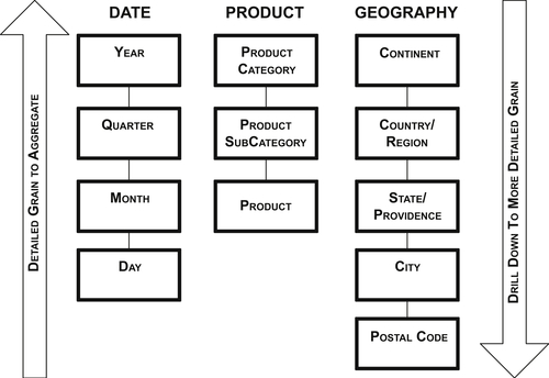
Many dimensions are hierarchical. Figure 10.1 shows some examples:
• Calendar date, which goes from year to a quarter, to month, and ending with day.
• Product, which goes from product category, breaking out into product subcategory, and ending with product.
• Geography, which goes from continent, to country, state, city, and ending with postal code.
FIGURE 10.1Hierarchies.
As the figure illustrates, data is aggregated from the most detailed level of data (i.e., the lowest level in the hierarchy up to the highest level). Typically, dashboards and reports initially display aggregated data, and business people drill down to greater levels of detail. Drilling up and down is moving along the hierarchies to examine the level of detail needed for the business analysis.
From a data modeling perspective, hierarchies are cascading series of many-to-one relationships at different levels. Each level corresponds to a dimension attribute. The hierarchies document relationships across levels. In an entity relationship (ER) model, each of these attributes would be an entity unto itself.
Dimensional models have three types of hierarchies: balanced, ragged, and unbalanced. It’s important to understand the differences and how to approach them in a dimensional model.
Balanced Hierarchies
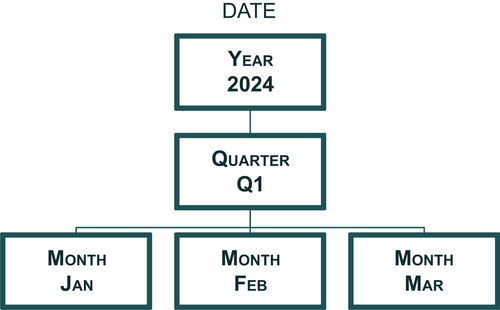
The balanced hierarchy is the simplest of these three hierarchies. (It is sometimes called a fixed hierarchy.) In it, all dimensional branches have the same number of levels—the same consistent depth with a consistent parent–child relationship. Enterprises create a balanced hierarchy to group and aggregate data within dimensions. It’s not unusual to have more than one balanced hierarchy within a dimension.
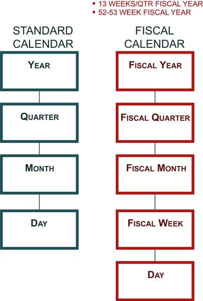
Figure 10.2 illustrates a balanced hierarchy. In this example, a year breaks down to a quarter, breaking down to months. An actual date would be the highest level of detail and lowest level in the hierarchy. The date dimension in Figure 10.3 illustrates a dimension with multiple hierarchies. In this example, an enterprise has a fiscal calendar that begins on July 1 and has a 4-4-5-quarter (4weeks for fiscal months 1 and 2, and 5weeks assigned to fiscal month 3.) This type of fiscal calendar enables an enterprise such as a retailer to analyze current versus previous periods in a more meaningful way for its business. Because the fiscal weeks are aligned with fiscal months, the fiscal hierarchy will include the fiscal week level that cannot be included in the standard calendar hierarchy because weeks do not align with standard weeks. Both of these hierarchies could be represented in the same dimension (as covered in the section on calendar dimensions in Chapter 9) with the lowest grain for both being a date.
FIGURE 10.2Date dimension.
FIGURE 10.3Standard and fiscal calendar hierarchies.
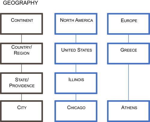
Ragged Hierarchies
A ragged hierarchy has the parent member of at least one member in the hierarchy that is not in the level immediately above it. In short, levels are skipped in the hierarchy. Both ragged and unbalanced hierarchies have branches with varying depths.
A typical example, as shown in Figure 10.4, is a geography or sales territory dimension. In the example, one branch has the continent of North America, country of United States, state of Illinois, and city of Chicago. The other branch has Europe as the continent, Greece as the country, and Athens as the city, but there is no state that is applicable to this dimension. In this example, each branch has a different depth and one branch has a gap, making this a ragged hierarchy.
If there is a limited number of levels and gaps in a hierarchy, then the pragmatic approach to handling aggregating data is to treat it as a balanced hierarchy. Depending on how the business wishes to handle the missing values, there are two options for what to populate in the missing attributes, just be sure to not use NULL in either case:
• An agreed-upon default value. In this example, that could be “not applicable” or “no state.”
• The value of the level above the gap. In this example, “Greece” would be used as the State attribute.
FIGURE 10.4Ragged hierarchies.
Both approaches allow the business to perform analyses with the same hierarchy for all the data examined. It’s the classic and easiest way to handle it.
If the hierarchy has many levels and gaps then use the approach discussed in handling variable depth hierarchies.
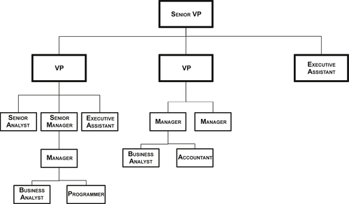
Unbalanced Hierarchies
Unbalanced hierarchies occur when the dimensional branches have varying numbers of levels—inconsistent depths while still having a consistent parent-child relationship.
The classic example, as shown in Figure 10.5, is an organizational chart. In the example, as we traverse through a senior vice president’s organization, the reporting relationships among employees vary widely. The organizational structure is unbalanced, with some branches in the hierarchy having more levels than others, the number of employees at each level varies, and employee titles are not uniform across a level. But there is always a parent–child relationship until the branch encounters a leaf node, such as an employee without anyone reporting to him or her. Obviously, an enterprise organizational chart would be much bigger than this, but it would still show a large amount of variation in the levels of the organization.
FIGURE 10.5Unbalanced hierarchies.
Working with Variable-Depth Hierarchies
The term variable-depth hierarchy refers to both unbalanced and ragged hierarchies. From a visual point of view, it is easy to see that the hierarchy is unbalanced or ragged. But it’s a little more complicated from the data modeling and processing points of view, either with SQL, ETL, or a BI tool. For accurate results, you need to understand and implement your approach to handling these various levels and not simply leave it up to the BI tool to aggregate and drill down by using the hierarchy levels.
The two approaches to handling unbalanced and ragged hierarchies are recursive pointer and bridge table.
Recursive Pointer
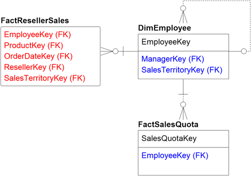
A recursive pointer is frequently used for handling a variable-depth hierarchy in dimensional modeling, but it has some serious drawbacks. This approach embeds a parent–child relationship in the dimension itself. The example in Figure 10.6 shows the dimension DimEmployee. The EmployeeKey is the primary key and child in the parent–child relationship, whereas the ManagerKey is the parent in the relationship and links back to the dimensional key itself. In a business context, the employee EmployeeKey points to the manager ManagerKey. The intent of this parent–child relationship is to recreate the organization chart in Figure 10.5.
A big drawback of the recursive pointer approach is that without custom coding, neither BI tools nor standard SQL can navigate from the top to bottom or vice versa in the hierarchy. And, if a ragged hierarchy is combined with an unbalanced hierarchy, which is common in financial charts of accounts, the added complexity of dealing with missing levels overwhelms these tools.
Figure 10.6 also illustrates how the fact tables, FactRellerSales and FactSalesQuota, are linked to the employee dimension table DimEmployee by using the foreign key EmployeeKey. The intent of the relationship is to determine which employee was responsible for a sale along with his or her sales quota, and then use the recursive relationship to aggregate the measures up to the top person in the organizational chart. You would only be able to perform the aggregation with custom coding and not with BI tools or standard SQL.
FIGURE 10.6Employee recursive example.
Bridge Table
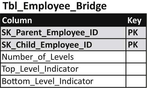
The second approach to handling variable depth hierarchies, which happens to be the best practice, is to create a bridge table that enables the relationships between the dimension and facts. A bridge table template design is depicted in Figure 10.7. The bridge table’s columns are:
• SK_Parent_Employee_ID—This is the parent identifier. It is paired with SK_Child_Employee_ID as a combination primary key.
• SK_Child_Employee_ID—This is the child identifier. It is paired with SK_Parent_Employee_ID as a combination primary key.
• Number_of_Levels—This is the number of levels from the parent (top level)
• Top_Level_Indicator—This is a flag indicating if this is the top level.
• Bottom_Level_Indicator—This is a flag indicating if this is the bottom level.
The issue with this approach is that it adds complexity to the model; it’s generally too complex for business people to manipulate directly. But the reality is that complexity is added because it’s needed. Sometimes dimensional modeling constructs are not easily completed using Microsoft Excel or some other business end-user tool. That’s why BI and online analytical processing (OLAP) tools, which understand relationships, are used in these more complex cases.
FIGURE 10.7Bridge table example.
When implementing a bridge table for an unbalanced hierarchy, it’s important to look at how to use it to navigate between the fact and the dimension. There are two ways to navigate:
• Traversing down from the top level numbers to the detailed numbers.
• Traversing up from the detailed data to more summarized data.
Traversing down using the example in Figure 10.8, would look like this:
• Start with FactResellerSales.
• Record SalesEmployeeKey, which is the salesperson’s employee identification.
• Next is the dimension DimEmployee, which lists all the employees in the company, their first name, last name, title, department number, and all their attributes as well as the sales territory key and the salesperson flag indicating they are salespeople.
• In the middle is the sales hierarchy bridge, which gives the parent employee key SK_Parent_Employee_ID, and the child employee key, SK_Child_Employee_ID, along with the total number of levels. There is a top level indicator, typically yes or no, and a bottom level indicator, also typically yes or no.
FIGURE 10.8Bridge table navigation.
• When you’re going down in aggregation, the fact joins the parent key level (remember, the data has already been aggregated). Then the dimension joins the child key row; then you move down into the lower level of detail.
Traversing up in the detailed data using the same example would look like this:
• The level of grain is the sale transaction, which includes the employee who made the sale.
• FactResellerSales joins the hierarchy of the child key row with foreign key SK_Child_Employee_ID.
• Then the dimension Dim_Employee joins the parent key SK_Parent_Employee_ID of the sales hierarchy bridge.
• That gets us the salesperson’s manager.
• So, the salesperson is the child, the manager is the parent. Then you can do a tree walk up the employee levels.
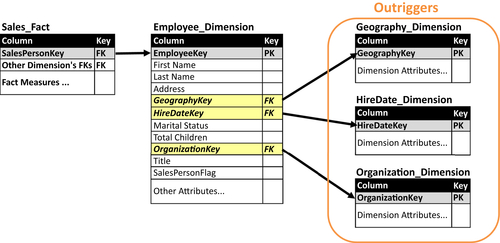
Outrigger Tables
The classic star schema has facts linked to dimensions without any relationship between dimensions themselves. Modeling an enterprise, however, is never that clear-cut and there are several conditions when dimensions link to other dimensions. We have discussed two of these conditions: snowflakes and bridges; the third condition is outriggers.
Outriggers are used when a dimension is referenced within another dimension. When a dimension is being designed, often all the attributes that are related to each other are gathered into that dimension. Further inspection reveals groups of attributes that are populated by different sources, at different times and for different purposes. In an ER model, they would be different entities.
Figure 10.9 depicts an employee dimension that is linked to three outriggers: geography, hire date, and organization dimensions. In the initial design of the employee dimension, some of the outriggers’ attributes may have been part of that dimension until more detailed review uncovered that these attributes should remain in their respective dimensions to be referenced by the employee dimension.
Using outriggers eliminates the need to redundantly store and update dimensional attributes in multiple locations. An example of this would have occurred if the attributes, such as a department’s name, manager, and size, were placed in the employee dimension rather accessing them in the organization dimension via a foreign key.
FIGURE 10.9Dimension outriggers.
Slowly Changing Dimensions
Dimensions have attributes that change over time. Products change price, cost, and composition. Employees are promoted, fired, change departments, and get new titles. Customers change addresses and names, get married or divorced, and move into different income brackets. These changes occur infrequently and unpredictably.
A business’s operational and transaction processing applications keep dimensional tables updated to the most current values to support ongoing business processes. Operational applications do not track changes to dimensional values because transactions only need the most current values. In addition, operational reporting uses data from the point in time that the transaction occurred, which is referred to as either “as was” or “as transacted.”
As you shift from operational to management analysis, however, the business needs to examine the facts (transactions and business events), not only in the context of the dimensional values at that point in time (“as was”), but also in the context of what the fact would look like if it occurred now with the current values of dimensions (“as is”). The capability to use either the “as was” or “as is” context is critical in business analysis such as examining trends, comparing period-versus-period performance and creating predictive models.
In the past, without formal techniques to track dimensional value changes, enterprises either ignored tracking (and lost any possibility to perform “as is” analysis) or they restated their facts by overwriting “as was” dimensional values with current values creating an “as is” state. Restating numbers was a time-consuming and messy technique that made it impossible to analyze facts “as was.” Losing the visibility to examine “as was” values made this approach a nonstarter.
Based on the need for a business to analyze both “as was” and “as is” states, several techniques referred to as types were created in dimensional modeling to record these changes and manage SCD:
• SCD type 0: Keep original
• SCD type 1: Overwrite existing data (row) with new data
• SCD type 2: Create a new row for new values
• SCD type 3: Track changes using separate columns but overwrite rest
• SCD type 4: Add mini-dimension
• SCD type 5: Combine types 4+1
• SCD type 6: Combines types 1+2+3 (=6)
• SCD type 7: Use both types 1+2
The type you choose depends on business analytic needs. Consider if and how you capture the dimensional changes to help decide what approach will work best.
There are several implementation considerations you need to make when selecting SCD techniques that you will use:
• First, will you apply the SCD techniques to all your dimensions equally or just to some of the dimensions? If you choose to treat certain dimensions differently, then you need to make sure that data integration developers, BI developers and business BI consumers are aware of and handle the difference when performing their work.
• Second, although it is often convenient to handle all dimensions in the same way, you typically can’t do this with individual dimensional attributes because they are definitely not created equally. For example, you might need to track historical values of the attributes for people (customer, prospect, or employee) or business demographics despite the current value being sufficient for many other attributes. No matter what SCD type you have chosen for the dimensions themselves, you should only apply those techniques to the attributes where there is business value in doing so; the remaining attributes only need to be updated as their value changes, and don’t need historical tracking.
• Finally, if you are tracking historical changes, you should only deploy those historical values to the business analytical processes that need it; the remaining analytical processes should get only the current view of the dimensions. This rule of thumb avoids adding complexity, confusion and processing overhead to the analytical processes that don’t need historical tracking.
SCD Type 0: Keep Original
The type 0 technique writes the original dimension record but then never updates it, regardless of any changes to dimensional attributes. This is the least likely technique to be used because businesses require, at a minimum, the most current dimension values, such as data about their customers, products, and employees.
SCD Type 1: Overwrite Existing Data
The type 1 technique is to overwrite historical values of dimensional attributes with the most current values. This technique keeps the dimensional values current, but disregards previous values. It is relatively straightforward to implement.
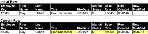
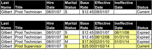
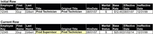
The example in Figure 10.10 shows the initial and current states of a row in the employee dimension listing the attributes for Guy Gilbert: his hire date of August 1, 2007, his title, base pay rate, and marital status. When the row was initially entered, Gilbert was a production technician, single, and paid $12.45 per hour. The current values in the row show that he is still single, paid $25.00 per hour, and is a production supervisor.
FIGURE 10.10Employee dimension—SCD type 1.
FIGURE 10.11SCD type 1 schema template.
There are two shortcomings to this technique:
• First, although we get the latest version of the dimensions, we lose the ability to track the history of the attributes. So we have no idea when the employee was promoted, when he was married or divorced, or when his base rate pay increased. In fact, his salary could easily have gone up multiple times, maybe even annually, but with this technique we don’t see any of that information.
• Second, if we have aggregated the data in summary tables or in OLAP cubes, we will have to reaggregate it because the underlying detailed data of the aggregation has changed.
This technique, particularly in the early years of data warehousing, was the most common way to deploy SCD. Reporting was limited to “as is” analysis, but at that time that was sufficient for many businesses because data warehousing was giving them the first effective approach to analyze their enterprise’s data outside application silos.
Type 1 Schema
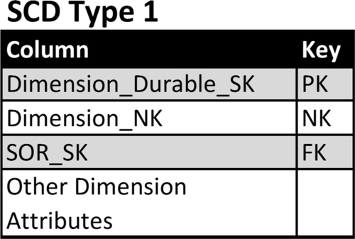
Figure 10.11 depicts a template schema supporting the SCD type 1 technique. The template columns show:
• Dimension_Durable_SK: This is the surrogate key used as the primary key for this dimension. This column is referred to as the durable, supernatural, or durable supernatural key. The term durable is used because the key values that are assigned to a dimension will continue to be used regardless of any changes in the values in the systems of record (SOR). The term supernatural is used to distinguish the key as independent from the SOR natural key.
• Dimension_NK: This is the natural key from the SOR. This column has the data type of the SOR if there is only one SOR or if all the SORs have the same data type. If there are multiple source systems with different data types, then use a data type such as a character string that can store all the natural keys’ values.
• SOR_SK: If the dimension has multiple SORs, such as a product dimension obtaining product lists from multiple source systems, then the SOR_SK is the foreign key linking to the SOR dimension depicted in Figure 10.11.
• Dimension attributes: There are one or more columns providing the values of all the attributes that the business needs to track.
Although we have differentiated dimensions’ surrogate keys from the source systems’ natural keys, there is an exception to this rule. This exception occurs when there is a single SOR for the dimension and that SOR generates a surrogate key as its primary key for that dimension. In this instance, the Dimension_Durable_SK should be the same as the Dimension_NK, eliminating the need to have the three key columns from the template in the dimension.
A word of caution: if the enterprise adds more SORs in the future (e.g., if a merger or acquisition occurs), then use the dimension template in Figure 10.10.
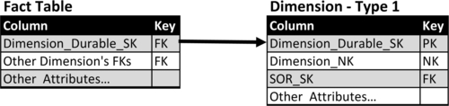
In the type 1 technique, fact tables linked to a dimension table use the foreign key. For example, see Dimension_Durable_SK in Figure 10.12.
SOR Dimension
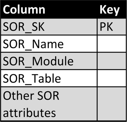
Figure 10.13 depicts a template for a system of record dimension that lists information regarding the source systems used to populate dimensions. The template columns show:
• SOR_SK: The surrogate key identifying the source system.
• SOR_Name: A name identifying the source system, typically an application name.
FIGURE 10.12Fact table links to SCD type 1 dimension.
FIGURE 10.13SOR dimension.
• SOR_Module and SOR_Table: If there is a need to identify SOR granularity greater than SOR_Name, then add these two columns to the dimension. For example, the SOR_Name identifies an application, the SOR_Module identifies a module within the application, and the SOR_Table lists the table the data is obtained from.
• SOR_Attributes: There are one or more columns providing the values of all the attributes that the enterprise needs to track.
SCD Type 2: Create New Row
The type 2 technique creates a new row in the dimension table every time a change occurs in an attribute that we wish to track. Unlike type 1, it enables you to track history accurately, so you see every time an attribute changes in that row and for that employee, as shown in Figure 10.14. It enables both “as is” and “as was” analysis.
This technique keeps track of all the historical changes in the dimension, allowing you to use the values of the dimension attributes at any point in time and examine the impact of those changes on the relevant fact tables. For example, if you’re looking at sales of specific products, you can look at what their retail price or production cost was at the point of sale and examine the impact of price or cost changes that occurred since.
This “as is” and “as was” analysis allows you to support trending analysis and period-over-period analysis. The only way you can look at trends, or be able to do year-over-year or quarter-over-quarter analysis, is to really look at apples versus apples, not apples versus oranges.
For example, suppose that the sales organization has reorganized, or a product has been regrouped into different categories and you then need to project sales trends of product sales by sale group. You would want to use the sales organization and product dimensions with their current values “as is” rather than what they were at the point of sale (“as was”). If you’re examining sales for financial performance analysis, however, you would keep the dimensional values at the time of sale “as was.” The type 2 technique enables the business to switch the dimensional values based on the type of analysis being performed.
Choosing whether or not to recast history (meaning, do you want to reshape the way you look at history based on as it is now or not?) will be a business decision. Often, if you keep the details in the type 2 dimension, this applies to your aggregations, so you need to decide if you want to recast your aggregations the way things are now or leave them the way they were before.
FIGURE 10.14Create new row.
Type 2 Schema
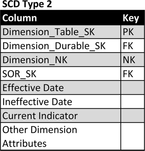
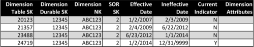
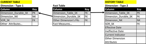
Figure 10.15 depicts a template schema supporting the SCD type 1 technique and Figure 10.16 provides example values. The template columns show:
• Dimension_Table_SK: This is the surrogate key used as the primary key for this dimension. Create a new row every time any of the dimensions have attributes that change. This key cannot be used to identify a specific dimension, such as a particular product or customer.
• Dimension_Durable_SK: This is the durable key for the dimension, such as a product or customer that uniquely identifies that dimension but does not provide uniqueness in this type 2 table if there have been changes to the dimension’s attribute.
• Dimension_NK: As with SCD type 1, this is the natural key from the SOR. This column has the data type of the SOR if there is only one SOR or if all the SORs have the same data type. If there are multiple source systems with different data types, then use a data type such as a character string that can store all the natural keys’ values.
• SOR_SK: As with SCD type 1, if the dimension has multiple SORs, such as a product dimension obtaining product lists from multiple source systems, then the SOR_SK is the foreign key linking to the SOR dimension depicted in Figure 10.11.
• Effective Date: This is the date that this row became effective and is used as the attribute value.
• Ineffective Date: This is the date this row’s attribute values become ineffective. If this is the row that contains the current attribute values but the ineffective date is unknown (i.e., this row is active until an attribute values changes), then some people use a NULL in this column; however, the best practice is to input a specific date far in the future, such as 12/31/9999, to avoid queries using a NULL in the selection criteria.
FIGURE 10.15SCD type 2 template.
FIGURE 10.16SCD type 2 schema template example.
• Current Indicator: This is a flag indicating this is the current version of the attribute values for a particular dimension. Typically, the current flag is the first value from one of these Boolean pairs: Y/N, 1/0, or T/F. Although some people use NULL for the values that are not current, it is best practice to use the second value in the Boolean pair examples to avoid queries using a NULL in the selection criteria.
• Dimension Attributes: As with SCD type 1, there are one or more columns providing the values of all the attributes that the business needs to track.
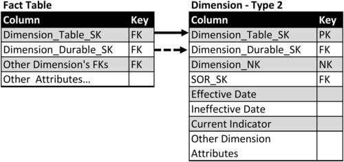
In the type 2 technique, fact tables linked to a dimension table include two foreign keys: Dimension_Table_SK and Dimension_Durable_SK as depicted in Figure 10.17. This enables business analysis to select the dimensional values for the following different timeframes:
• To get the values at the point of time that the fact occurred “as was,” select the row based on Dimension_Table_SK.
• To get the current values, select the row based on Dimension_Durable_SK and where the Currrent_Indicator=“Y” (or whatever flag was used to indicate it is the current row).
• To get the value at any particular point in time, select the row based on Dimension_Table_SK with the date of interest being between the effective date and ineffective date.
FIGURE 10.17Fact table links to SCD type 2 dimension.
Another useful analysis that can be performed regarding timeframes is the future or “what will be.” There are instances when an enterprise may know future costs they will incur because of contracts they have negotiated with suppliers or create product prices that will take effect in the future. In those circumstances, the attributes can be input into their respective dimensions with future effective date, and the business can perform what-if analysis using the future dates.
SCD Type 3: Track Changes Using Separate Columns but Overwrite the Rest
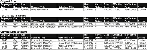
With the SCD type 3 technique, you continue to overwrite the rows as in type 1, but you add a new attribute in the row for a particular attribute that’s important for the business to track. Generally, you keep track of the new or current value of that particular attribute as well as the original or the previous value in separate fields at the time of change.
The example in Figure 10.18 shows the same employee as previous examples. We want to track the employee’s current title and his original title when hired. The initial row shows the employee attributes at the time of hire. The current row has the current values of the employee attributes but, just as with type 1, we have no visibility to what attributes have changed with the exception of the attributes that were added to support type 3. In our example, we selected the title as the attribute we’re tracking, so we have both the current title, production supervisor, as well as the original title, production technician.
FIGURE 10.18Employee dimension—SCD type 3.
Although type 3 is not as commonly used as other SCD techniques, it is very useful in specific business conditions such as health care and financial services:
In health care, the contracts between providers and insurance companies reflect annual changes to prices insurers will pay for procedures. There’s often a significant lag, however, in processing and paying claims in health care, resulting in payments being made on the previous year’s contract. So, payment processes may need to look at either current or previous prices because of the late-arriving facts—claims that come in for past year that need to use the past year’s prices. In that particular case, the attribute that we’re tracking is price; we keep track of both the current and previous year’s contract prices in type 3 attributes.
In financial services, it is sometimes important to track the original bank branch or account representative that a customer engaged with when opening an account, getting a mortgage or securing a loan rather than the current branch or account representative.
When comparing the SCD type 2 and 3 techniques, consider what happens if the intermediate values are lost and you cannot accurately track history. You can look at some attributes and do some comparisons, but in general, you’re in the same position as you are with type 1: you can’t perform both “as is” or “as was” analysis.
Type 3 Schema
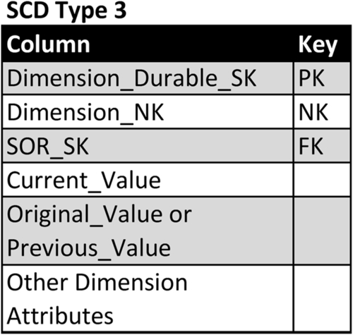
Figure 10.19 depicts a template schema supporting the SCD type 3. The template columns:
• Dimension_Durable_SK: as with type 1, this is the surrogate key used as the primary key for this dimension. This column is referred to as the durable, supernatural, or durable supernatural key. The term durable is used because the key values that are assigned to a dimension will continue to be used regardless of any changes in the values in the SOR. The term supernatural is used to distinguish the key as independent from the SOR natural key.
• Dimension_NK: as with SCD type 1, this is the natural key from the SOR. This column has the data type of the SOR if there is only one SOR or if all the SORs have the same data type. If there are multiple source systems with different data types, then use a data type such as a character string that can store all the natural keys’ values.
• SOR_SK: as with SCD type 1, if the dimension has multiple SORs, such as a product dimension obtaining product lists from multiple source systems, then the SOR_SK is the foreign key linking to the SOR dimension depicted in Figure 10.11.
• Current_Value: The current values of the attribute using the type 3 technique.
• Original_Value or Previous_Value: Either the original or previous value of the attribute using the type 3 technique.
• Other Dimension Attributes: as with SCD type 1, there are one or more columns providing the values of all the attributes that the business needs to track.
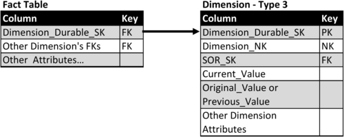
With the type 3 technique, fact tables linked to a dimension table use the foreign key. For example see Dimension_Durable_SK in Figure 10.20.
FIGURE 10.19SCD type 3 template.
FIGURE 10.20Fact table links to SCD type 3 dimension.
SCD Type 4: Add Mini-Dimension
Although we characterize dimensional attributes as changing slowly over time, there are instances when they change more frequently. These attributes are referred to as rapidly- or volatile changing dimensions. When rapidly changing dimensions are encountered and dimensional tables are relatively large in respect to the total number of rows, then these attributes may adversely affect both loading data and BI query performance.
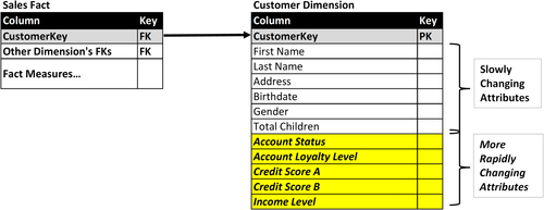
The example in Figure 10.21 shows a customer dimension that has both slowly and rapidly changing attributes. The slowly changing attributes are:
• First and last name
• Address
• Marital status
• Birthday (should not change but may be corrected or filled in when initially NULL)
• Number of children
The more rapidly changing attributes are:
• Account status
• Account loyalty level
• Various credit scores
• Income level
FIGURE 10.21Customer dimension with both slowly and rapidly changing attributes.
With the SCD type 4 technique, the approach is to divide the slowly and rapidly changing attributes into two groups. The first group contains the SCD and is regarded as the primary or base dimension. The second group, referred to as a profile, contains the more rapidly changing dimensions that are put into a mini-dimension.
Multiple Mini-Dimension Approaches
As with many dimensional modeling techniques, there are mini-dimension variations used to address specific business processes or analytical scenarios. These approaches are split, multiple, and banded-value, as described below:
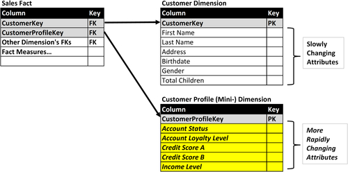
Split approach—single mini-dimension. The most common approach is to simply put the dimensions into primary and mini-dimension tables. Any fact tables that link to the split dimension would have foreign keys linked to these two tables.
Figure 10.22 depicts the customer dimension shown in Figure 10.21 split into two tables: Customer dimension and Customer profile dimension (mini-dimension.) We have retained the original foreign key, CustomerKey, in the Sales Fact, but now have the primary key from the mini-dimension, CustomerProfileKey, as an additional foreign key.
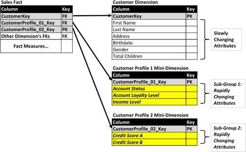
Multiple approach—multiple mini-dimensions. There are circumstances in which there are subgroups of rapidly changing attributes that behave in a similar manner. The subgroups may be updated at similar frequencies and times, or by common business processes. Under these circumstances, it is often beneficial from a processing perspective to split each subgroup into its own mini-dimension as portrayed in Figure 10.23. The relevant fact tables have foreign keys to the primary dimension table and all the mini-dimensions.
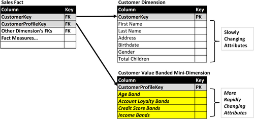
Banded-value approach. This technique with mini-dimensions is useful when the rapidly changing attributes in the customer dimension are numeric values such as credit scores, account loyalty levels and income levels. Under these conditions, you define segmentation bands that group a range of values together. This reduces the amount and frequency of changes in the segmentation bands. Figure 10.24 depicts our customer mini-dimension example that has been altered to store banded values, such as age, account loyalty, credit score, and income rather than the underlying numeric values. This is a way to avoid frequent changes because, for example, you have an income range instead of specific income numbers. You only have to update the record if the person goes above or below the threshold for that band. The primary risk with this approach is that once you lose the detail you are forced to stay with this segmentation even if business conditions or analytical needs change. There is a discussion of value-band dimensions later in this chapter.
FIGURE 10.22Customer dimension example split into primary and mini-dimensions.
FIGURE 10.23Customer dimension example with multiple mini-dimensions.
FIGURE 10.24Customer dimension example with value-banded mini-dimensions.
Mini-Dimensions Need Outrigger
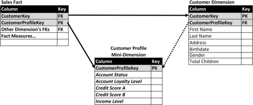
The classic design for SCD type 4 with a mini-dimension has the fact table storing the foreign keys to the primary and mini-dimensions, but no relationship between the dimensions themselves. That reminds me of the phrase, stereotypically attributed to the state of Maine, where the traveler asks a local resident for directions and is told “You can’t get there from here.” (Or, with a Maine accent: “You can’t get theyah from heah.”) That answer is no more helpful to the traveler than it is to the BI consumers. With the classic design, your only way to relate the primary and mini-dimensions is through a fact table as an intermediary, which has the following drawbacks:
• Slow query performance both in updating dimensions and BI queries.
• Redundant combinations are returned in join queries based on how many times the dimension tables are referenced in the fact table.
• Gaps will exist where a primary dimension will not be able to connect with its associated mini-dimension because neither is referenced in a fact table.
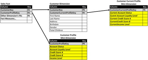
The best practice is to place a foreign key to the mini-dimension in the primary dimension as depicted in Figure 10.25 where CustomerProfileKey links the customer dimension to the customer profile mini-dimension.
FIGURE 10.25Mini-dimension as outrigger.
SCD Type 5: Combine Types 4+1
The SCD type 5 technique builds upon the type 4 technique by splitting the dimension into a primary dimension with the slowly changing attributes and a mini-dimension with the rapidly changing attributes. It then grafts the type 1 technique of storing a current copy of the mini-dimension attributes. The technique is referred to as type 5 because it is the combination of types 4+1.
There are several approaches to implementing type 5:
• Create a separate mini-dimension that contains the current values of the rapidly changing attributes as depicted in Figure 10.26. The primary dimension, Customer Dimension, contains the foreign key, CustomerCurrentProfileKey, to the second mini-dimension, Customer Current Profile Mini-Dimension.
• The second mini-dimension, Customer Current Profile Mini-Dimension in our example, is actually a view created from the first mini-dimension, Customer Profile Mini-Dimension using a Current_Indicator attribute that is present in type 2 dimensions (which both the primary and first mini-dimensions are.)
FIGURE 10.26Customer example type 5 with second mini-dimension.
FIGURE 10.27Customer dimension example with hybrid mini-dimensions.
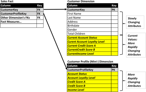
• In the third approach, place the current values of each of the rapidly changing attributes in the primary dimension table. Figure 10.27 depicts the customer dimension with each attribute in the mini-dimension (account status, account loyalty level, etc.) having corresponding attributes in the primary dimension with the current values (current account status, current account loyalty level, etc.).
Use this approach when most of the business analysis with this dimension is going to use the current value in “as is” reporting. The primary dimension contains all the current values of the attributes supporting “as is” queries, whereas “as was” queries, assumed to be infrequent, use the mini-dimension that tracks the historical values.
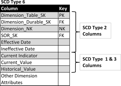
SCD Type 6: Combine Types 1+2+3 (=6)
The SCD type 6 technique blends portions of SCD types 2, 1, and 3. Similar to type 2, a type 6 schema creates a new record with every change in attribute values that are being tracked. The current value (type 1) of a specific attribute is added as a column (type 3) onto every row. This allows rows to be filtered or grouped by either the current or historical value of the type 3 column. The type 2 portion of this technique enables “as is” and “as was” analysis.
Figure 10.28 depicts an employee dimension using the type 6 technique. The example shows three different states of the dimension’s rows for a specific employee: original row when the employee is hired, the first time the employee’s attributes are changed—he or she got married, received a promotion and salary increase, and the current state of his or her employee records listing all the changes in title, marital status and salary. As with the type 2 technique, the effective and ineffective dates of each row are recorded along with a current status indicator. The Historical Title column lists his or her title during the effective time period, whereas the Current Title is always updated to reflect the current title.
FIGURE 10.28Employee example SCD type 6.
Type 6 Schema
Figure 10.29 depicts a template schema supporting the SCD type 6 technique. See the descriptions for the SCD type 2 columns in the section “Type 2 schema” earlier in this chapter, as they are the same in this schema:
• Dimension_Table_SK
• Dimension_Durable_SK
• Dimension_NK
• SOR_SK
• Effective Date
• Ineffective Date
• Current Indicator
• Dimension Attributes
FIGURE 10.29SCD type 6 schema.
The blended SCD types 3 and 1 techniques are provided by the following columns:
• Current_Value: The current value of the attribute being tracked. This value is applied to this column in all rows associated with the durable key.
• Historical_Value: The value of the attribute being tracked at the point in time that the row was initially created. This value does not change once it has been input into its row.
SCD Type 7: Use both Types 1+2
SCD type 7 technique creates both type 1 and type 2 versions of a dimension. From a data perspective, with this technique you accurately track all the historical changes to dimensional attributes that the business requires. From a business analysis perspective, you have the option to either expose the historical values in the type 2 dimension for both “as was” and “as is” analysis or provide current values from the type 1 dimension for “as is” analysis. The benefit of offering both is that when only “as is” is needed query performance and business productivity are greatly increased. Because a considerable portion of business analysis will be “as is,” these benefits will occur often.
Most businesses need to have historically accurate dimensional data. They want to be able to track history, perform “as is” and “as was” reporting, and meet industry and governmental regulatory requirements. Most common business queries, analytics, and reports, however, only require current values. The vast majority of reports that people create on a daily basis are just looking at “as is” conditions. How many customers do I have? What are my sales? What are my costs related to the state of the dimensions at that particular time? This is type 1 data, and query performance is fast because you only have one unique row in each dimension.
It gets more complicated, however, when you have type 2 data. Rather than one row for an employee or product in a dimension, you have many rows tracking all the changes over time. Now the queries are very complex, and it’s time-consuming to actually select the rows within the dimensions because you have to specify time periods, the durable keys, and any other attributes by which you need to filter. And, you may have dozens of dimensions that you want to select and join with the fact table. Each of these queries has to use ineffective and effective dates in order to accomplish and pick out the right dates.
This problem required a solution that would let you get the best of both worlds: track historical data in type 2 processing and get type 1 query performance. The hybrid approach tracks the dimensions in type 2, slowly changing dimension processes within the data warehouse, and then exposes a type 1 view of that as a source of most queries, reports, and analysis. That view is available in data marts and OLAP cubes. You can also implement it either as a table that just has the type 1 version of the type 2 dimension or you can use some database constructs like materialized views, indexed partitions, or simple database views in order to create the type 1 view of the type 2 data—in which case, any queries that just need “as is” reporting would not have to look at the effective and ineffective dates for the current flags.
I recommend the SCD type 7 technique as the best pragmatic approach to capturing historical values and then matching the appropriate schema for the business analysis that is going to be performed. You only need to provide current values (type 1). It greatly simplifies querying, lessens the chance for errors, and improves understanding. As an aside, this technique is used by some of the Master Data Management vendors.
The SCD type 7 technique goes by many other names:
• SCD type 4—this was its first name until the numbers were shuffled around
• SCD hybrid approach
• Current and history table approach
Type 7 Schema
Figure 10.30 depicts a schema supporting the SCD type 7 technique. There are three types of tables involved: fact, current (type 1), and history (type 2).
FIGURE 10.30SCD type 7 schema.
The history table includes the SCD type 2 columns (see “Type 2 Schema” earlier in this chapter) and contains all the entire history of attribute changes for the dimension. As with type 2, the schema has these columns:
• Dimension_Table_SK
• Dimension_Durable_SK
• Dimension_NK
• SOR_SK
• Effective Date
• Ineffective Date
• Current Indicator
• Dimension Attributes
The current table also includes the SCD type 1 columns (see “Type 1 schema” earlier in this chapter) and only contains the most current rows of the dimension’s attributes. The standard convention is to prefix the names of the attribute columns from the history table with the string of “current_” to differentiate the current and history attributes. The schema includes:
• Dimension_Durable_SK
• Dimension_NK
• SOR_SK
• Dimension Attributes
Some people will add the SCD type 2 attributes—Dimension_Table_SK, Effective_Date, and Ineffective_Date—but if it is not needed for the business analysis, then that goes against the reason why the current table is being used.
There are two alternatives: (1) creating and updating two tables—history and current—by using data integration, or (2) using the database to create a view or a materialized view.
Causal Dimension
Facts have obvious attributes such as product, customer, geography, and time. This is the “who, what, where” of the fact. But facts also have a “why” component. This is the causal dimension. (Not to be confused with “casual.”) The causal dimension tells you why a customer bought or returned a product. Examples of causal relationships include promotions, campaigns, and the reason for sales and returns.
This can be very important information, but often these relationships are overlooked in the initial design of a dimensional model; they are looked at as degenerate dimensions, meaning they’re just some piece of information about the fact that we don’t need to store. They tend to be overlooked when promotion or campaign data is being stored somewhere outside of the enterprise application that is the primary source system feeding the dimensional model, such as in a campaign tool or a separate database. This, in effect, hides the attributes and dimensions from the source system you’re actually pulling data from.
Likewise, reason codes—reasons why people buy, exchange or return products—typically aren’t in the initial source system either, causing them to be overlooked. These reason codes can be essential for sales and marketing analytics on customers behavior, so bringing this data into view is very important.
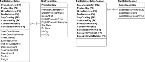
Figure 10.31 shows two casual dimensions: DimPromotion and DimSalesReason.
On the left side, the fact table FactInternetSales with the foreign key PromotionKey, links to the casual dimension DimPromotion, which has attributes such as promotion name, item discount amount, promotion type, category, start and end dates, and quantities for that promotion. With this promotion dimension, the business can track the effectiveness of the promotion, view trends for different types of promotions, and undertake related analytics.
FIGURE 10.31Causal dimension examples.
The fact table FactSalesReason has the foreign key SalesReasonKey that links to the casual dimension DimSalesReason, which has the attributes for why somebody bought or returned a product. These reasons might be captured by a call center worker, by a salesperson, or online in a survey. The information provided by the causal dimensions is invaluable to the marketing and sales analytics.
Multivalued Dimensions
When you start to encounter more complicated data situations that require advanced data modeling techniques, you may need to use a multivalued dimension situation. These kinds of situations arise when a fact measurement is associated with multiple values in a dimensional table. This is opposed to the more typical scenario, in which a fact measurement is associated with one value in a dimension, allowing a normal fact and dimensional star schema.
Health care is a common real-world example of multivalued dimensions. A patient arrives at the emergency room after a vertigo episode caused him to fall and break his arm. He will have at least two diagnoses—vertigo and broken arm—and will require several types of treatments for the vertigo and setting the broken bone. The hospital has diagnostic codes for each ailment and procedure codes for each treatment. The hospital must track all of the codes for this patient’s visit and any subsequent visits.
Insurance and financial accounts provide another example. It is common for financial accounts and certain types of insurance policies to be associated with two account owners or policy holders. One account will have multiple types of products or accounts associated with the owners, such as checking, savings, a mortgage, and a credit card. It’s a many-to-many relationship between the account owners and the products in their account.
There are three typical approaches to handling these complicated data situations:
• Pick one value, ignore others
• Extend the attributes
• Create a bridge table
Pick One Value, Ignore Others
Picking one specific value and ignoring the other values is the quick and dirty approach. With this, our normal relationships between dimensions and facts stay intact and our BI tools can handle that kind of construct.
The problem, of course, is that if you pick one specific value and ignore the others, you lose all the other details. If the details aren’t needed, such as if you’re just looking to get an insurance claim paid, you might have a business rule that you only need one value upon which to get paid. This would be a viable situation. But a hospital, on the other hand, would need to track all the different diagnostic and procedure codes that went along with a patient’s medical condition, whether the claim is paid for one value or not.
Extend the Attributes
The second approach, which I’ve seen many times, is to actually extend the dimension attributes to include a fixed number of multivalue dimensions. In essence, this creates a list within the dimensional row. For example, the hospital could assume no one will have more than 10 diagnoses, so you would put in 10 columns, one for each code (or make it 20 to add a buffer). It’s a quick way to solve the problem when you can assume that there is an upper bound to the number of times that an attribute can occur.
The problem with this approach is that it’s limited by the context of the upper bound, and, more importantly, that you’re imposing a repeating group into your dimensional row. That causes problems when you want to look at the total number of diagnostic codes, for example, and how many instances there are of a particular diagnostic code.
Bridge Table
The third solution, building a bridge table, is the most sophisticated approach for multivalued dimensions and produces the most complete results. As the name implies, it bridges the gap between the fact and dimension tables.
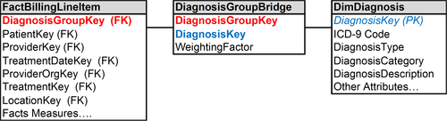
The bridge table needs to support the many-to-many relationships between a fact table and associated dimensions. The example in Figure 10.32 depicts:
• Fact table:FactBillingLineItem with information about the patient, about the provider (doctor), treatment date, what organization the doctor is from, other key information such as treatment and location. It contains the foreign key DiagnosisGroupKey that links to the bridge table.
FIGURE 10.32Bridge table approach.
• Bridge table:DiagnosisGroupBridge with the DiagnosisGroupKey that is used to group the set of diagnoses that a patient encountered in a visit to a provider (i.e., a row in the fact table), the foreign key DiagnosisKey linking to the dimension table, and a weighting factor (discussed in the following section).
• Dimension table:DimDiagnosis with a primary key of DiagnosisKey and several types of medical terms or categorizations that are applicable to that diagnosis.
A bridge table has a weighting factor if all the members of the DiagnosisGroupKey are not considered equal and are determined by a predefined weighting. The weighting factor allocates numeric additive facts. In this example, the weighting factor is the method to sum up the additive attributes associated with specific diagnosis. Typically the weighting factor adds up to one. In the example, this relates to one visit to the doctor. There is a certain percentage weighting factor adding up to one for one to N number of rows for the different diagnostic keys. Sometimes these weighting factors will be described in medical health care provider situations, there are formulas they use for other cases where this is marketing or sales, when they come up with the weighting or allocations.
There are two types of queries with a bridge table:
• Queries with a weighting factor to allocate the values. For example, based on a health care insurers’ contract, a health care provider, such as the doctor, will use the weighting factors when “scoring” (i.e., aggregating attributes from the diagnosis dimension).
• Queries without a weighting factor to allocate the values. In this scenario, the health care provider treats each diagnosis equally and aggregates the diagnosis dimension’s attributes without applying any weighting factor. There is no weighting factor to determine the total number of occurrences of a diagnosis regardless of how many diagnoses for the patient. Suppose you want to know how many times, for example, swine flu was diagnosed. That would be one occurrence in multiple group keys. So you ignore the weighting factor; in this case, you’re just trying to get the total number of diagnosis keys.
Using the bridge allows you to perform analysis of facts and dimensions with a many-to-many relationship. It also enables the ability to treat the relationships equally or, as so often happens because the relationships are not all equal, to use a weighting factor based on business rules.
Junk Dimensions
Perhaps you have a junk drawer in your kitchen where you put miscellaneous things that you know you’ll need some day, but you’re not sure where else to put them. Dimensional modeling has a junk drawer too, and it also manages clutter and helps make things more productive. Junk dimensions are a way to handle the multitude of low-cardinality transactions, system codes, flags, identifiers, and text attributes by putting them into one table so you can better manage them.
It is typical for these miscellaneous flags to have 2–10 possible values. Sometimes they are yes or no attributes, whereas other times they are a short list of options to complete a business transaction.
JUNK, GARBAGE, CROSS-REFERENCE
Many information technology people hate the name junk (or garbage) dimension because they do not want to tell their business people that they are creating junk. These are also called “cross-reference dimensions”—this is the term I prefer to use with clients. The term junk dimension, however, is well-recognized in the industry, so we use it here to avoid confusion.
Table 10.1
Junk Dimension Alternatives That Don’t Work Well
Alternatives
Results
Put them into an existing dimension
Does not fit because attributes have different grain. Creates Cartesian product
Leave them in the fact table
Too cluttered, row size too large, affects speed, cannot be conformed
Make them into separate dimensions
Overly complex with too many tables, affects speed and maintenance
Eliminate them
Cannot eliminate if used by business group and needed in analytics
Misguided Attempts
As shown in Table 10.1, there are four misguided ways people attempt to approach the problem of these miscellaneous flags:
• First, they put them into an existing dimension. Force-fitting doesn’t work when the attributes are different grains or if it creates a Cartesian product and makes the dimension too large.
• Second, leave them in a fact table. This common, misguided approach makes the fact table cluttered and the row sizes very large; it also slows down performance and makes it so the dimensions cannot be conformed.
• Third is to make them into separate dimensions. It takes out code fields and puts the attributes into their own dimension tables. Although this is much better than the first two approaches, it creates many, many tables with a small number of rows, 10 rows for example. This negatively affects speed because you’re always doing queries and joins to these many small tables. It increases maintenance because there are so many tables to maintain. It is much better, however, than hand-coding the flags in your applications because it makes them visible and documented.
• Fourth, is to just eliminate them. Then they can’t be used by the business, which is a problem if they are needed for analytics.
Recommended Solution
The solution to these numerous miscellaneous flags, codes, or indicator fields from the transactional systems is to create a junk dimension, and then to use views similar to role-playing dimensions when necessary. In essence, it takes the third option mentioned previously, which is generating numerous tables to have these values, and putting together or collapsing them into one junk dimension.
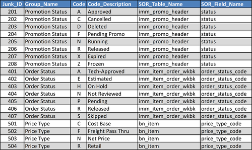
FIGURE 10.33Junk dimension example.
The dimension consists of low-cardinality columns, such as flags, codes, indicators, and text attributes, meaning there are not too many values. These values rarely change, but there may be no correlation between the groups of these attributes within the junk dimension.
This is a pragmatic approach because it takes the best attributes of the large number of tables and puts them into one location to be managed, updated, and queried upon. The primary function of this junk table is to enable filtering reporting. It prevents these attributes from being embedded in the report code, and it enables a much better documentation of the system.
In the example in Figure 10.33, code fields and their descriptions are grouped together based on common usage and input into a junk dimension. The columns in this example are:
• Junk_ID—surrogate key
• Group_Name—a set of common code fields
• Code—list of code fields
• Code_Descriptions—textual description displayed for the codes
• SOR_Table_Name—table from source system from which these codes are obtained
• SOR_Field_Name—field in table from which these codes are obtained
These code fields are often used for filtering and grouping data in reporting. A BI application such as a dashboard or interactive report might provide pick lists or pull-down menus using the groupings and codes as the options presented. Creating a junk dimension replaces hard-coded options in applications, makes it easier to maintain and change these codes, and increases the ability to reuse and share because these codes are in tables rather than embedded in code or personal spreadsheets.
Value Band Reporting
It is common in reporting and analytics to group data together. You group the facts by a particular dimension or fact measurement. When grouping by a dimension, you may have a hierarchy, which is a natural group. When grouping a product that has a subcategory and a category together, you could aggregate on each of those levels.
But grouping fact measures, especially numbers, is not so easy or efficient. Often the range of numbers is hard-coded into a report, making it impossible to make changes to that band or even document what that band is. So the best practice is to create value band groupings for particular fact measures.
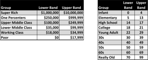
The two examples in Figure 10.34 are for income and age. The income column includes bands from the US Census Bureau: super rich, rich, upper middle class, lower middle class, working class, and poor. (That is the Census Bureau’s wording, not mine!) The age column has bands for age groups: infant, elementary, high school, college, young adult, 30s, 40s, 60s, and really old. Both have a lower and upper band.
The examples show that two different groups or kinds of analysis might need to group income levels differently. They might have more groups of income levels, smaller groups of income levels, and based on international settings, have different numbers based on whether it’s Canada, the United States, or Europe. The same applies to the age groupings. If you’re selling toys, you might have a fine-grained age band for younger people and may not care about anyone over the age of 12.
If you’re looking at social security and retirement benefits, you might have everybody grouped under 30 in one band, and more do fine-grained tuning of people over 60. There is a lot of room for variation in these group bands, so it’s best practice to put these bands into tables, rather than hard coding them into reports.
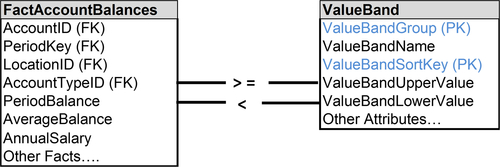
Rather than hard-code value bands in reports, you should use a value band table for analysis. Figure 10.35 depicts an example where a fact table, Fact_Account_Balances, uses the value band dimension, Value_Band_Dimension, to group accounts by ranges of account balances. The value band dimension contains the following:
• ValueBandGroup: Primary key
• ValueBandName: Name used to describe the band, such as super rich and poor in the previous example. This column would be used for filtering, sorting, and grouping accounts in reports.
FIGURE 10.34Value band reporting.
FIGURE 10.35Value band reporting approaches.
• ValueBandSortKey: Often the ValueBandName does not sort in the order that business people prefer, so this numeric column would be used to obtain the preferred order.
• ValueBandUpperValue: The upper bound of the range in this value band.
• ValueBandLowerValue: The lower bound of the range in this value band.
When assigning accounts to value bands, the account’s PeriodBalance, for example, is compared with the value band upper and lower values.
This example allows numerous value bands for age and income depending on who wants to look at the numbers. It lets you change the bands without having to change the fact table.
It’s also possible to take a hybrid approach, where you follow the first approach, which is to create the value band table and put the foreign key in the fact table, but then keep the original fact measure in the balance table so you can do numeric calculations directly on the detail. You can do either direct numeric analysis or the value band analysis in your dimensional model.
Heterogeneous Products
Heterogeneous products and services can present some challenges with dimensional models. When you have diverse sets of products and customers, you can simply have multiple facts and dimensions. For example, General Electric sells light bulbs to customers, jet engines to the airline industry, and gas turbines to utilities. It’s not a common set of customers; it’s a diverse set of customers and diverse products.
It’s more complicated, however, when a company sells diverse products to a common set of customers. How do you represent these diverse products and services as one fact in situations like the following:
• Multiline insurance companies sell distinct products—life, auto, property, and casualty insurance to the same customer.
• Financial services companies have retail banks, commercial banking, credit cards, mutual funds, 401k plans, and many other financial instruments, all targeted to the same customer. These products have facts and dimensions that are very different from one another.
• High-tech companies sell hardware, software, training, maintenance, and services to a common customer base, but they have different facts with very different measures and attributes.
Enterprises can take various approaches to handle heterogeneous products sold to a common set of customers. The first one, however, is something you should avoid:
• Merge attributes into a single fact table. This results in large fact tables with rows that have many empty values. It gets to be a very complex fact table that’s being updated by multiple lines of business and usually there are many coordination problems. This approach is not recommended.
• Create separate dimensions in fact tables representing the diverse businesses. This is viable if they are totally separate businesses. That, however, is typically not the case if they are trying to sell to a common base of customers. Even if you have separate dimensions in the fact tables, you still need some set of financial consolidation in the company because you have to report to the government, and you need to look at your overall enterprise financials. This approach may not be applicable.
• Create a single dimension and a single fact table representing a set of core attributes or measures. This approach works when there are common measures such as financial data used in corporate finance, regulatory reporting, and senior management looking at the performance metrics of the enterprise. It uses fact and dimension tables that are specific to the diverse products or businesses that can then be linked to the core tables. This recommended approach is a hybrid solution that, from a pragmatic point of view, has been highly effective in representing heterogeneous products.
Alternate Dimensions
The classic assumption is that facts are connected to a set of conformed dimensions, meaning that all business analysis uses the same definition and hierarchy of a specific dimension. That implies that there is only one way to group customers or products, for example. But this attempt to create conformity inhibits the ability to create customized views of dimensions to match the analytical requirements of business functions and processes. Finance, marketing, sales, and manufacturing may have legitimate business needs to group customers and products differently.
When one standard dimension is available for business analysis, then the burden is shifted to business people to create the alternative views of the dimensions. This is typically done by extracting data to spreadsheets to enable analysis using alternative versions of dimensions that were created manually by business people. Not only is this a productivity drain, but there is no documentation, sharing is haphazard, and the potential for inconsistency is high.
Dimensional models need to accommodate alternative views of dimensions to support business needs, improve productivity, and provide consistency. There are two basic approaches:
• Hot swappable dimensions (also called profile tables)
• Custom dimension groups
Hot Swappable Dimension
Hot swappable dimensions are switched at query-time based on business needs. They got their name because someone thought it was analogous to hot swappable hardware components that are switched in real time.
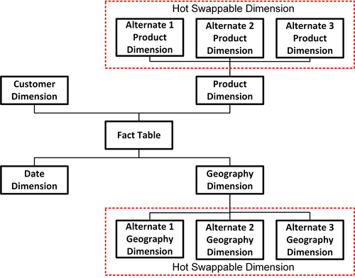
Hot swappable dimensions are implemented by connecting a fact table with alternate versions of a dimension, then using one alternative for analysis at query time. The alternative is either selected by the business person explicitly or automatically by the BI application based on specific business rules. Figure 10.36 depicts an example of hot swappable dimensions used for both the product and geography dimensions. The product and geography dimensions in this example are each considered to be conformed dimensions. Each of the alternatives is a variation based on:
• Having a subset of the conformed dimension attributes
• Filtering the rows from the conformed dimensions
• Creating a different hierarchy or grouping of the dimensions
FIGURE 10.36Hot swappable dimension example.
If hot swappable dimensions are a subset of the rows and columns in the conformed dimensions but do not provide alternate hierarchies, then they can be implemented as either tables or views. However, with alternate hierarchies, physical tables are required.
Custom Dimension Groups
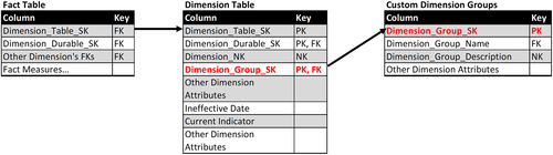
The second approach to creating alternative dimensions is to enhance the dimension’s schema to accommodate different dimensional groups.
As depicted in Figure 10.37, an additional dimension is created, Custom_Dimension_Groups that has a row for each alternate grouping with descriptive attributes. The new dimension could be used as a filter to select alternates during query time or to create views that would be made available to specific groups of business people. The foreign key Dimension_Group_SK is added to the dimension table. The primary key for the dimension table is a combination of Dimension_Table_SK, Dimension_Durable_SK, and Dimension_Group_SK.
FIGURE 10.37Alternate dimension groups.
Fact tables are not modified, however, and continue to be linked to the dimension table using the Dimension_Table_SK as the foreign key.
Too Few or Too Many Dimensions
When you complete your first iteration of a dimensional model, you might find that you have too few or too many dimensions. It is common to have 6–18 dimensions to model a business process. Although there will be common or conformed dimensions across business processes, it is likely that as the number of processes modeled grows, so too will the number of dimensions.
If you have too few, consider if any of these are missing:
• Outriggers
• Role-playing dimensions
• Causal dimensions
• Multivalued dimensions and bridge tables
• Value band tables
It’s possible to add any of these after you enter into the production phase of your dimensional model because they don’t affect the existing primary and foreign keys in your dimensional model. Keep in mind, however, that striving to develop a comprehensive a model early will improve productivity and analytical capabilities.
If you end up with far too many dimensions, such as hundreds, for example, then you need to determine if you have any of these issues:
• Some of the dimensions are dependent on each other and need to be combined. If there is a one-to-one mapping they definitely need to be combined.
• There are degenerate dimensions, which need to be collapsed as talked about in Chapter 9.
• Many of the dimensions are really an accumulation of junk dimensions that could be put into one table to improve management and productivity.