6. Special Numbers

Some sequences of numbers arise so often in mathematics that we recognize them instantly and give them special names. For example, everybody who learns arithmetic knows the sequence of square numbers 1, 4, 9, 16, . . .. In Chapter 1 we encountered the triangular numbers 1, 3, 6, 10, . . .; in Chapter 4 we studied the prime numbers 2, 3, 5, 7, . . .; in Chapter 5 we looked briefly at the Catalan numbers 1, 2, 5, 14, . . ..

In the present chapter we’ll get to know a few other important sequences. First on our agenda will be the Stirling numbers and , and the Eulerian numbers ; these form triangular patterns of coefficients analogous to the binomial coefficients in Pascal’s triangle. Then we’ll take a good look at the harmonic numbers H_n, and the Bernoulli numbers B_n; these differ from the other sequences we’ve been studying because they’re fractions, not integers. Finally, we’ll examine the fascinating Fibonacci numbers F_n and some of their important generalizations.

6.1 Stirling Numbers

We begin with some close relatives of the binomial coefficients, the Stirling numbers, named after James Stirling (1692–1770). These numbers come in two flavors, traditionally called by the no-frills names “Stirling numbers of the first and second kind.” Although they have a venerable history and numerous applications, they still lack a standard notation. Following Jovan Karamata, we will write for Stirling numbers of the second kind and for Stirling numbers of the first kind; these symbols turn out to be more user-friendly than the many other notations that people have tried.

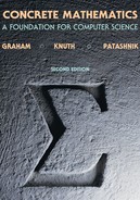
Tables 258 and 259 show what and look like when n and k are small. A problem that involves the numbers “1, 7, 6, 1” is likely to be related to , and a problem that involves “6, 11, 6, 1” is likely to be related to , just as we assume that a problem involving “1, 4, 6, 4, 1” is likely to be related to ; these are the trademark sequences that appear when n = 4.

“. . . par cette notation, les formules deviennent plus symétriques.”

—J. Karamata [199]

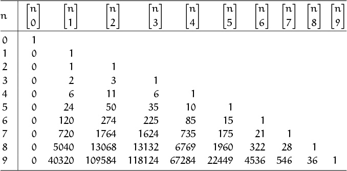
Stirling numbers of the second kind show up more often than those of the other variety, so let’s consider last things first. The symbol stands for the number of ways to partition a set of n things into k nonempty subsets. For example, there are seven ways to split a four-element set into two parts:

(Stirling himself considered this kind first in his book [343].)

thus . Notice that curly braces are used to denote sets as well as the numbers . This notational kinship helps us remember the meaning of , which can be read “n subset k.”

Let’s look at small k. There’s just one way to put n elements into a single nonempty set; hence , for all n > 0. On the other hand , because a 0-element set is empty.

The case k = 0 is a bit tricky. Things work out best if we agree that there’s just one way to partition an empty set into zero nonempty parts; hence . But a nonempty set needs at least one part, so for n > 0.

What happens when k = 2? Certainly . If a set of n > 0 objects is divided into two nonempty parts, one of those parts contains the last object and some subset of the first n – 1 objects. There are 2^n–1 ways to choose the latter subset, since each of the first n – 1 objects is either in it or out of it; but we mustn’t put all of those objects in it, because we want to end up with two nonempty parts. Therefore we subtract 1:

(This tallies with our enumeration of ways above.)

A modification of this argument leads to a recurrence by which we can compute for all k: Given a set of n > 0 objects to be partitioned into k nonempty parts, we either put the last object into a class by itself (in ways), or we put it together with some nonempty subset of the first n – 1 objects. There are possibilities in the latter case, because each of the ways to distribute the first n – 1 objects into k nonempty parts gives subsets that the nth object can join. Hence

This is the law that generates Table 258; without the factor of k it would reduce to the addition formula (5.8) that generates Pascal’s triangle.

And now, Stirling numbers of the first kind. These are somewhat like the others, but counts the number of ways to arrange n objects into k cycles instead of subsets. We verbalize ‘’ by saying “n cycle k.”

Cycles are cyclic arrangements, like the necklaces we considered in Chapter 4. The cycle

can be written more compactly as ‘[A, B, C, D]’, with the understanding that

[A, B, C, D] = [B, C, D, A] = [C, D, A, B] = [D, A, B, C];

a cycle “wraps around” because its end is joined to its beginning. On the other hand, the cycle [A, B, C, D] is not the same as [A, B, D, C] or [D, C, B, A].

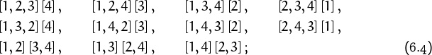
There are eleven different ways to make two cycles from four elements:

“There are nine and sixty ways of constructing tribal lays, And-every-single-one-of-them-is-right.”

—Rudyard Kipling

hence .

A singleton cycle (that is, a cycle with only one element) is essentially the same as a singleton set (a set with only one element). Similarly, a 2-cycle is like a 2-set, because we have [A, B] = [B, A] just as {A, B} = {B, A}. But there are two different 3-cycles, [A, B, C] and [A, C, B]. Notice, for example, that the eleven cycle pairs in (6.4) can be obtained from the seven set pairs in (6.1) by making two cycles from each of the 3-element sets.

In general, n!/n = (n – 1)! different n-cycles can be made from any n-element set, whenever n > 0. (There are n! permutations, and each n-cycle corresponds to n of them because any one of its elements can be listed first.) Therefore we have

This is much larger than the value we had for Stirling subset numbers. In fact, it is easy to see that the cycle numbers must be at least as large as the subset numbers,

because every partition into nonempty subsets leads to at least one arrangement of cycles.

Equality holds in (6.6) when all the cycles are necessarily singletons or doubletons, because cycles are equivalent to subsets in such cases. This happens when k = n and when k = n – 1; hence

In fact, it is easy to see that

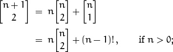
(The number of ways to arrange n objects into n – 1 cycles or subsets is the number of ways to choose the two objects that will be in the same cycle or subset.) The triangular numbers = 1, 3, 6, 10, . . . are conspicuously present in both Table 258 and Table 259.

We can derive a recurrence for by modifying the argument we used for . Every arrangement of n objects in k cycles either puts the last object into a cycle by itself (in ways) or inserts that object into one of the cycle arrangements of the first n – 1 objects. In the latter case, there are n – 1 different ways to do the insertion. (This takes some thought, but it’s not hard to verify that there are j ways to put a new element into a j-cycle in order to make a (j + 1)-cycle. When j = 3, for example, the cycle [A, B, C] leads to

[A, B, C, D],     [A, B, D, C],     or     [A, D, B, C]

when we insert a new element D, and there are no other possibilities. Summing over all j gives a total of n – 1 ways to insert an nth object into a cycle decomposition of n – 1 objects.) The desired recurrence is therefore

This is the addition-formula analog that generates Table 259.

Comparison of (6.8) and (6.3) shows that the first term on the right side is multiplied by its upper index (n–1) in the case of Stirling cycle numbers, but by its lower index k in the case of Stirling subset numbers. We can therefore perform “absorption” in terms like and , when we do proofs by mathematical induction.

Every permutation is equivalent to a set of cycles. For example, consider the permutation that takes 123456789 into 384729156. We can conveniently represent it in two rows,

1 2 3 4 5 6 7 8 9
3 8 4 7 2 9 1 5 6,

showing that 1 becomes 3 and 2 becomes 8, etc. The cycle structure comes about because 1 becomes 3, which becomes 4, which becomes 7, which becomes the original element 1; that’s the cycle [1, 3, 4, 7]. Another cycle in this permutation is [2, 8, 5]; still another is [6, 9]. Therefore the permutation 384729156 is equivalent to the cycle arrangement

[1, 3, 4, 7] [2, 8, 5] [6, 9].

If we have any permutation π₁π₂ . . . π_n of {1, 2, . . . , n}, every element is in a unique cycle. For if we start with m₀ = m and look at m₁ = π_m0, m₂ = π_m1, etc., we must eventually come back to m_k = m₀. (The numbers must repeat sooner or later, and the first number to reappear must be m₀ because we know the unique predecessors of the other numbers m₁, m₂, . . . , m_k–1.) Therefore every permutation defines a cycle arrangement. Conversely, every cycle arrangement obviously defines a permutation if we reverse the construction, and this one-to-one correspondence shows that permutations and cycle arrangements are essentially the same thing.

Therefore is the number of permutations of n objects that contain exactly k cycles. If we sum over all k, we must get the total number of permutations:

For example, 6 + 11 + 6 + 1 = 24 = 4!.

Stirling numbers are useful because the recurrence relations (6.3) and (6.8) arise in a variety of problems. For example, if we want to represent ordinary powers xⁿ by falling powers xⁿ, we find that the first few cases are

x⁰ = x⁰;
x¹ = x¹;
x² = x² + x¹;
x³ = x³ + 3x² + x¹;
x⁴ = x⁴ + 6x³ + 7x² + x¹.

These coefficients look suspiciously like the numbers in Table 258, reflected between left and right; therefore we can be pretty confident that the general formula is

We’d better define when k < 0 and n ≥ 0.

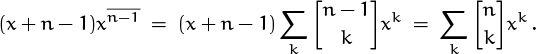
And sure enough, a simple proof by induction clinches the argument: We have x·x^k = x^k+1 + kx^k, because x^k+1 = x^k(x – k); hence x·x^n–1 is

In other words, Stirling subset numbers are the coefficients of factorial powers that yield ordinary powers.

We can go the other way too, because Stirling cycle numbers are the coefficients of ordinary powers that yield factorial powers:

We have (x + n – 1)·x^k = x^k+1 + (n – 1)x^k, so a proof like the one just given shows that

This leads to a proof by induction of the general formula

(Setting x = 1 gives (6.9) again.)

But wait, you say. This equation involves rising factorial powers , while (6.10) involves falling factorials . What if we want to express in terms of ordinary powers, or if we want to express xⁿ in terms of rising powers? Easy; we just throw in some minus signs and get

This works because, for example, the formula

x⁴ = x(x – 1)(x – 2)(x – 3) = x⁴ – 6x³ + 11x² – 6x

is just like the formula

= x(x + 1)(x + 2)(x + 3) = x⁴ + 6x³ + 11x² + 6x

but with alternating signs. The general identity

of exercise 2.17 converts (6.10) to (6.12) and (6.11) to (6.13) if we negate x.

Also, , a generalization of (6.9).

We can remember when to stick the (–1)^n–k factor into a formula like (6.12) because there’s a natural ordering of powers when x is large:

The Stirling numbers and are nonnegative, so we have to use minus signs when expanding a “small” power in terms of “large” ones.

We can plug (6.11) into (6.12) and get a double sum:

This holds for all x, so the coefficients of x⁰, x¹, . . . , x^n–1, xⁿ⁺¹, xⁿ⁺², . . . on the right must all be zero and we must have the identity

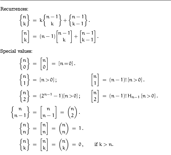
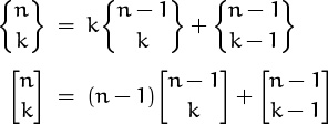
Stirling numbers, like binomial coefficients, satisfy many surprising identities. But these identities aren’t as versatile as the ones we had in Chapter 5, so they aren’t applied nearly as often. Therefore it’s best for us just to list the simplest ones, for future reference when a tough Stirling nut needs to be cracked. Tables 264 and 265 contain the formulas that are most frequently useful; the principal identities we have already derived are repeated there.

When we studied binomial coefficients in Chapter 5, we found that it was advantageous to define for negative n in such a way that the identity is valid without any restrictions. Using that identity to extend the ’s beyond those with combinatorial significance, we discovered (in Table 164) that Pascal’s triangle essentially reproduces itself in a rotated form when we extend it upward. Let’s try the same thing with Stirling’s triangles: What happens if we decide that the basic recurrences

are valid for all integers n and k? The solution becomes unique if we make the reasonable additional stipulations that

In fact, a surprisingly pretty pattern emerges: Stirling’s triangle for cycles appears above Stirling’s triangle for subsets, and vice versa! The two kinds of Stirling numbers are related by an extremely simple law [220, 221]:

We have “duality,” something like the relations between min and max, between x and x, between and , between gcd and lcm. It’s easy to check that both of the recurrences and amount to the same thing, under this correspondence.

6.2 Eulerian Numbers

Another triangle of values pops up now and again, this one due to Euler [104, §13; 110, page 485], and we denote its elements by . The angle brackets in this case suggest “less than” and “greater than” signs; is the number of permutations π₁π₂ . . . π_n of {1, 2, . . . , n} that have k ascents, namely, k places where π_j < π_j+1. (Caution: This notation is less standard than our notations , for Stirling numbers. But we’ll see that it makes good sense.)

(Knuth [209, first edition] used for .)

For example, eleven permutations of {1, 2, 3, 4} have two ascents:

1324,     1423,     2314,     2413,     3412;
1243,     1342,     2341;         2134,     3124,     4123.

(The first row lists the permutations with π₁ < π₂ > π₃ < π₄; the second row lists those with π₁ < π₂ < π₃ > π₄ and π₁ > π₂ < π₃ < π₄.) Hence .

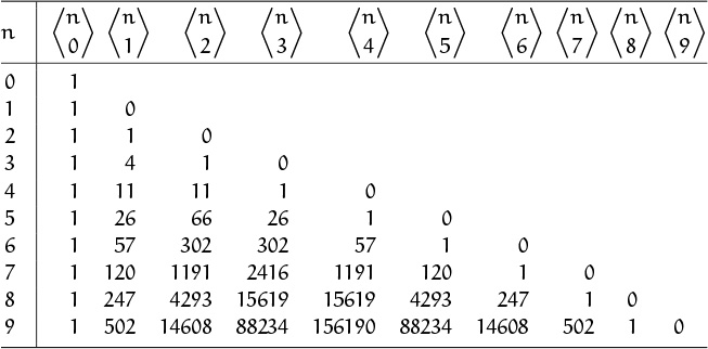
Table 268 lists the smallest Eulerian numbers; notice that the trademark sequence is 1, 11, 11, 1 this time. There can be at most n – 1 ascents, when n > 0, so we have on the diagonal of the triangle.

Euler’s triangle, like Pascal’s, is symmetric between left and right. But in this case the symmetry law is slightly different:

The permutation π₁π₂ . . . π_n has n–1–k ascents if and only if its “reflection” π_n . . . π₂π₁ has k ascents.

Let’s try to find a recurrence for . Each permutation ρ = ρ₁ . . . ρ_n–1 of {1, . . . , n – 1} leads to n permutations of {1, 2, . . . , n} if we insert the new element n in all possible ways. Suppose we put n in position j, obtaining the permutation π = ρ₁ . . . ρ_j–1 n ρ_j . . . ρ_n–1. The number of ascents in π is the same as the number in ρ, if j = 1 or if ρ_j–1 < ρ_j; it’s one greater than the number in ρ, if ρ_j–1 > ρ_j or if j = n. Therefore π has k ascents in a total of ways from permutations ρ that have k ascents, plus a total of ways from permutations ρ that have k – 1 ascents. The desired recurrence is

Once again we start the recurrence off by setting

and we will assume that when k < 0.

Eulerian numbers are useful primarily because they provide an unusual connection between ordinary powers and consecutive binomial coefficients:

(This is called “Worpitzky’s identity” [378].) For example, we have

Western scholars have recently learned of a significant Chinese book by Li ShanLan [249; 265, pages 320–325], published in 1867, which contains the first known appearance of formula (6.37).

and so on. It’s easy to prove (6.37) by induction (exercise 14).

Incidentally, (6.37) gives us yet another way to obtain the sum of the first n squares: We have , hence

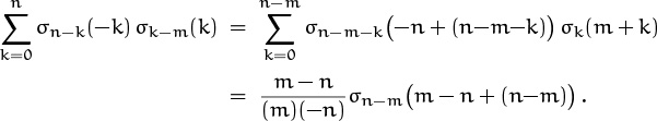
The Eulerian recurrence (6.35) is a bit more complicated than the Stirling recurrences (6.3) and (6.8), so we don’t expect the numbers to satisfy as many simple identities. Still, there are a few:

If we multiply (6.39) by z^n–m and sum on m, we get . Replacing z by z – 1 and equating coefficients of z^k gives (6.40). Thus the last two of these identities are essentially equivalent. The first identity, (6.38), gives us special values when m is small:

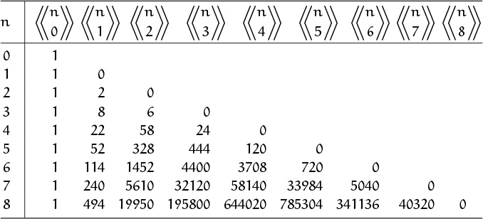
We needn’t dwell further on Eulerian numbers here; it’s usually sufficient simply to know that they exist, and to have a list of basic identities to fall back on when the need arises. However, before we leave this topic, we should take note of yet another triangular pattern of coefficients, shown in Table 270. We call these “second-order Eulerian numbers” , because they satisfy a recurrence similar to (6.35) but with n replaced by 2n – 1 in one place:

These numbers have a curious combinatorial interpretation, first noticed by Gessel and Stanley [147]: If we form permutations of the multiset {1, 1, 2, 2, . . . , n, n} with the special property that all numbers between the two occurrences of m are greater than m, for 1 ≤ m ≤ n, then is the number of such permutations that have k ascents. For example, there are eight suitable single-ascent permutations of {1, 1, 2, 2, 3, 3}:

113322, 133221, 221331, 221133, 223311, 233211, 331122, 331221.

Thus . The multiset {1, 1, 2, 2, . . . , n, n} has a total of

suitable permutations, because the two appearances of n must be adjacent and there are 2n – 1 places to insert them within a permutation for n – 1. For example, when n = 3 the permutation 1221 has five insertion points, yielding 331221, 133221, 123321, 122331, and 122133. Recurrence (6.41) can be proved by extending the argument we used for ordinary Eulerian numbers.

Second-order Eulerian numbers are important chiefly because of their connection with Stirling numbers [148]: We have, by induction on n,

For example,

(We already encountered the case n = 1 in (6.7).) These identities hold whenever x is an integer and n is a nonnegative integer. Since the right-hand sides are polynomials in x, we can use (6.43) and (6.44) to define Stirling numbers and for arbitrary real (or complex) values of x.

If n > 0, these polynomials and are zero when x = 0, x = 1, . . . , and x = n; therefore they are divisible by (x–0), (x–1), . . . , and (x–n). It’s interesting to look at what’s left after these known factors are divided out. We define the Stirling polynomials σ_n(x) by the rule

(The degree of σ_n(x) is n – 1.) The first few cases are

σ₀(x)   =   1/x ;
σ₁(x)   =   1/2 ;
σ₂(x)   =   (3x – 1)/24 ;
σ₃(x)   =   (x² – x)/48 ;
σ₄(x)   =   (15x³ – 30x² + 5x + 2)/5760 .

So 1/x is a polynomial?

(Sorry about that.)

They can be computed via the second-order Eulerian numbers; for example,

σ₃(x) = ((x–4)(x–5) + 8(x–4)(x+1) + 6(x+2)(x+1)) /6!.

It turns out that these polynomials satisfy two very pretty identities:

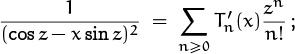
And in general, if S_t(z) is the power series that satisfies

then

Therefore we can obtain general convolution formulas for Stirling numbers, as we did for binomial coefficients in Table 202; the results appear in Table 272. When a sum of Stirling numbers doesn’t fit the identities of Table 264 or 265, Table 272 may be just the ticket. (An example appears later in this chapter, following equation (6.100). Exercise 7.19 discusses the general principles of convolutions based on identities like (6.50) and (6.53).)

6.3 Harmonic Numbers

It’s time now to take a closer look at harmonic numbers, which we first met back in Chapter 2:

These numbers appear so often in the analysis of algorithms that computer scientists need a special notation for them. We use H_n, the ‘H’ standing for “harmonic,” since a tone of wavelength 1/n is called the nth harmonic of a tone whose wavelength is 1. The first few values look like this:

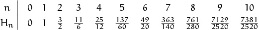
Exercise 21 shows that H_n is never an integer when n > 1.

Here’s a card trick, based on an idea by R. T. Sharp [325], that illustrates how the harmonic numbers arise naturally in simple situations. Given n cards and a table, we’d like to create the largest possible overhang by stacking the cards up over the table’s edge, subject to the laws of gravity:

This must be Table 273.

To define the problem a bit more, we assume that card k rests on card k + 1, for 1 ≤ k < n. We also require the right edge of each card to be parallel to the edge of the table; otherwise we could increase the overhang by rotating the cards so that their corners stick out a little farther. And to make the answer simpler, we assume that each card is 2 units long.

With one card, we get maximum overhang when its center of gravity is just above the edge of the table. The center of gravity is in the middle of the card, so we can create half a cardlength, or 1 unit, of overhang.

With two cards, it’s not hard to convince ourselves that we get maximum overhang when the center of gravity of the top card is just above the edge of the second card, and the center of gravity of both cards combined is just above the edge of the table. The joint center of gravity of two cards will be in the middle of their common part, so we are able to achieve an additional half unit of overhang.

This pattern suggests a general method, where we place cards so that the center of gravity of the top k cards lies just above the edge of the k + 1st card (which supports those top k). The table plays the role of the n + 1st card. To express this condition algebraically, we can let d_k be the distance from the extreme edge of the top card to the corresponding edge of the kth card from the top. Then d₁ = 0, and we want to make d_k+1 the center of gravity of the first k cards:

(The center of gravity of k objects, having respective weights w₁, . . . , w_k and having respective centers of gravity at positions p₁, . . . , p_k, is at position (w₁p₁ + · · · + w_kp_k)/(w₁ + · · · + w_k).) We can rewrite this recurrence in two equivalent forms

kdk+1	= k + d1 + · · · + dk–1 + dk ,          k ≥ 0 ;
(k – 1)dk	= k – 1 + d1 + · · · + dk–1 ,             k ≥ 1.

Subtracting these equations tells us that

kd_k+1 – (k – 1)d_k = 1 + d_k ,               k ≥ 1;

hence d_k+1 = d_k + 1/k. The second card will be offset half a unit past the third, which is a third of a unit past the fourth, and so on. The general formula

follows by induction, and if we set k = n we get d_n+1 = H_n as the total overhang when n cards are stacked as described.

Could we achieve greater overhang by holding back, not pushing each card to an extreme position but storing up “potential gravitational energy” for a later advance? No; any well-balanced card placement has

Furthermore d₁ = 0. It follows by induction that d_k+1 ≤ H_k.

Notice that it doesn’t take too many cards for the top one to be completely past the edge of the table. We need an overhang of more than one cardlength, which is 2 units. The first harmonic number to exceed 2 is , so we need only four cards.

Anyone who actually tries to achieve this maximum overhang with 52 cards is probably not dealing with a full deck—or maybe he’s a real joker.

And with 52 cards we have an H₅₂-unit overhang, which turns out to be H₅₂/2 ≈ 2.27 cardlengths. (We will soon learn a formula that tells us how to compute an approximate value of H_n for large n without adding up a whole bunch of fractions.)

An amusing problem called the “worm on the rubber band” shows harmonic numbers in another guise. A slow but persistent worm, W, starts at one end of a meter-long rubber band and crawls one centimeter per minute toward the other end. At the end of each minute, an equally persistent keeper of the band, K, whose sole purpose in life is to frustrate W, stretches it one meter. Thus after one minute of crawling, W is 1 centimeter from the start and 99 from the finish; then K stretches it one meter. During the stretching operation W maintains his relative position, 1% from the start and 99% from the finish; so W is now 2 cm from the starting point and 198 cm from the goal. After W crawls for another minute the score is 3 cm traveled and 197 to go; but K stretches, and the distances become 4.5 and 295.5. And so on. Does the worm ever reach the finish? He keeps moving, but the goal seems to move away even faster. (We’re assuming an infinite longevity for K and W, an infinite elasticity of the band, and an infinitely tiny worm.)

Metric units make this problem more scientific.

Let’s write down some formulas. When K stretches the rubber band, the fraction of it that W has crawled stays the same. Thus he crawls 1/100th of it the first minute, 1/200th the second, 1/300th the third, and so on. After n minutes the fraction of the band that he’s crawled is

So he reaches the finish if H_n ever surpasses 100.

We’ll see how to estimate H_n for large n soon; for now, let’s simply check our analysis by considering how “Superworm” would perform in the same situation. Superworm, unlike W, can crawl 50 cm per minute; so she will crawl H_n/2 of the band length after n minutes, according to the argument we just gave. If our reasoning is correct, Superworm should finish before n reaches 4, since H₄ > 2. And yes, a simple calculation shows that Superworm has only cm left to travel after three minutes have elapsed. She finishes in 3 minutes and 40 seconds flat.

A flatworm, eh?

Harmonic numbers appear also in Stirling’s triangle. Let’s try to find a closed form for , the number of permutations of n objects that have exactly two cycles. Recurrence (6.8) tells us that

and this recurrence is a natural candidate for the summation factor technique of Chapter 2:

Unfolding this recurrence tells us that ; hence

We proved in Chapter 2 that the harmonic series ∑_k1/k diverges, which means that H_n gets arbitrarily large as n → ∞. But our proof was indirect; we found that a certain infinite sum (2.58) gave different answers when it was rearranged, hence ∑_k 1/k could not be bounded. The fact that H_n → ∞ seems counter-intuitive, because it implies among other things that a large enough stack of cards will overhang a table by a mile or more, and that the worm W will eventually reach the end of his rope. Let us therefore take a closer look at the size of H_n when n is large.

The simplest way to see that H_n → ∞ is probably to group its terms according to powers of 2. We put one term into group 1, two terms into group 2, four into group 3, eight into group 4, and so on:

Both terms in group 2 are between and , so the sum of that group is between and . All four terms in group 3 are between and , so their sum is also between and 1. In fact, each of the 2^k–1 terms in group k is between 2^–k and 2^1–k; hence the sum of each individual group is between and 1.

This grouping procedure tells us that if 1/n is in group k, we must have H_n > k/2 and H_n ≤ k (by induction on k). Thus H_n → ∞, and in fact

We now know H_n within a factor of 2. Although the harmonic numbers approach infinity, they approach it only logarithmically—that is, quite slowly.

We should call them the worm numbers, they’re so slow.

Better bounds can be found with just a little more work and a dose of calculus. We learned in Chapter 2 that H_n is the discrete analog of the continuous function ln n. The natural logarithm is defined as the area under a curve, so a geometric comparison is suggested:

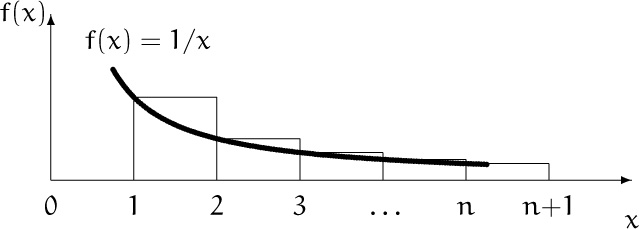
The area under the curve between 1 and n, which is , is less than the area of the n rectangles, which is . Thus ln n < H_n; this is a sharper result than we had in (6.59). And by placing the rectangles a little differently, we get a similar upper bound:

“I now see a way too how y^e aggregate of y^e termes of Musicall progressions may bee found (much after y^e same manner) by Logarithms, but y^e calculations for finding out those rules would bee still more troublesom.”

—I. Newton [280]

This time the area of the n rectangles, H_n, is less than the area of the first rectangle plus the area under the curve. We have proved that

We now know the value of H_n with an error of at most 1.

“Second order” harmonic numbers arise when we sum the squares of the reciprocals, instead of summing simply the reciprocals:

Similarly, we define harmonic numbers of order r by summing (–r)th powers:

If r > 1, these numbers approach a limit as n → ∞; we noted in exercise 2.31 that this limit is conventionally called Riemann’s zeta function:

Euler [103] discovered a neat way to use generalized harmonic numbers to approximate the ordinary ones, . Let’s consider the infinite series

which converges when k > 1. The left-hand side is ln k – ln(k – 1); therefore if we sum both sides for 2 ≤ k ≤ n the left-hand sum telescopes and we get

Rearranging, we have an expression for the difference between H_n and ln n:

When n → ∞, the right-hand side approaches the limiting value

which is now known as Euler’s constant and conventionally denoted by the Greek letter γ. In fact, ζ(r) – 1 is approximately 1/2^r, so this infinite series converges rather rapidly and we can compute the decimal value

“Huius igitur quantitatis constantis C valorem deteximus, quippe est C = 0, 577218.”

—L. Euler [103]

Euler’s argument establishes the limiting relation

thus H_n lies about 58% of the way between the two extremes in (6.60). We are gradually homing in on its value.

Further refinements are possible, as we will see in Chapter 9. We will prove, for example, that

This formula allows us to conclude that the millionth harmonic number is

H_1000000 ≈ 14.3927267228657236313811275 ,

without adding up a million fractions. Among other things, this implies that a stack of a million cards can overhang the edge of a table by more than seven cardlengths.

What does (6.66) tell us about the worm on the rubber band? Since H_n is unbounded, the worm will definitely reach the end, when H_n first exceeds 100. Our approximation to H_n says that this will happen when n is approximately

e^100–γ ≈ e^99.423 .

In fact, exercise 9.49 proves that the critical value of n is either e^100–γ or e^100–γ. We can imagine W’s triumph when he crosses the finish line at last, much to K’s chagrin, some 287 decillion centuries after his long crawl began. (The rubber band will have stretched to more than 10²⁷ light years long; its molecules will be pretty far apart.)

Well, they can’t really go at it this long; the world will have ended much earlier, when the Tower of Brahma is fully transferred.

6.4 Harmonic Summation

Now let’s look at some sums involving harmonic numbers, starting with a review of a few ideas we learned in Chapter 2. We proved in (2.36) and (2.57) that

Let’s be bold and take on a more general sum, which includes both of these as special cases: What is the value of

when m is a nonnegative integer?

The approach that worked best for (6.67) and (6.68) in Chapter 2 was called summation by parts. We wrote the summand in the form u(k)Δv(k), and we applied the general identity

Remember? The sum that faces us now, , is a natural for this method because we can let

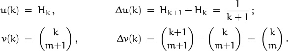
(In other words, harmonic numbers have a simple Δ and binomial coefficients have a simple Δ^–1, so we’re in business.) Plugging into (6.69) yields

The remaining sum is easy, since we can absorb the (k + 1)^–1 using our old standby, equation (5.5):

Thus we have the answer we seek:

(This checks nicely with (6.67) and (6.68) when m = 0 and m = 1.)

The next example sum uses division instead of multiplication: Let us try to evaluate

If we expand H_k by its definition, we obtain a double sum,

Now another method from Chapter 2 comes to our aid; equation (2.33) tells us that

It turns out that we could also have obtained this answer in another way if we had tried to sum by parts (see exercise 26).

Now let’s try our hands at a more difficult problem [354], which doesn’t submit to summation by parts:

(This sum doesn’t explicitly mention harmonic numbers either; but who knows when they might turn up?)

(Not to give the answer away or anything.)

We will solve this problem in two ways, one by grinding out the answer and the other by being clever and/or lucky. First, the grinder’s approach. We expand (n – k)ⁿ by the binomial theorem, so that the troublesome k in the denominator will combine with the numerator:

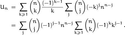
This isn’t quite the mess it seems, because the k^j–1 in the inner sum is a polynomial in k, and identity (5.40) tells us that we are simply taking the nth difference of this polynomial. Almost; first we must clean up a few things. For one, k^j–1 isn’t a polynomial if j = 0; so we will need to split off that term and handle it separately. For another, we’re missing the term k = 0 from the formula for nth difference; that term is nonzero when j = 1, so we had better restore it (and subtract it out again). The result is

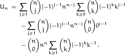
OK, now the top line (the only remaining double sum) is zero: It’s the sum of multiples of nth differences of polynomials of degree less than n, and such nth differences are zero. The second line is zero except when j = 1, when it equals –nⁿ. So the third line is the only residual difficulty; we have reduced the original problem to a much simpler sum:

For example, ; hence U₃ = 27(T₃ – 1) as claimed.

How can we evaluate T_n? One way is to replace by , obtaining a simple recurrence for T_n in terms of T_n–1. But there’s a more instructive way: We had a similar formula in (5.41), namely

If we subtract out the term for k = 0 and set x = 0, we get –T_n. So let’s do it:

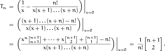
(We have used the expansion (6.11) of ; we can divide x out of the numerator because .) But we know from (6.58) that ; hence T_n = H_n, and we have the answer:

That’s one approach. The other approach will be to try to evaluate a much more general sum,

the value of the original U_n will drop out as the special case U_n(n, –1). (We are encouraged to try for more generality because the previous derivation “threw away” most of the details of the given problem; somehow those details must be irrelevant, because the nth difference wiped them away.)

We could replay the previous derivation with small changes and discover the value of U_n(x, y). Or we could replace (x + ky)ⁿ by (x + ky)^n–1(x + ky) and then replace by , leading to the recurrence

this can readily be solved with a summation factor (exercise 5).

But it’s easiest to use another trick that worked to our advantage in Chapter 2: differentiation. The derivative of U_n(x, y) with respect to y brings out a k that cancels with the k in the denominator, and the resulting sum is trivial:

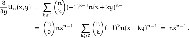
(Once again, the nth difference of a polynomial of degree < n has vanished.)

We’ve proved that the derivative of U_n(x, y) with respect to y is nx^n–1, independent of y. In general, if f′(y) = c then f(y) = f(0) + cy; therefore we must have U_n(x, y) = U_n(x, 0) + nx^n–1y.

The remaining task is to determine U_n(x, 0). But U_n(x, 0) is just xⁿ times the sum T_n = H_n we’ve already considered in (6.72); therefore the general sum in (6.74) has the closed form

In particular, the solution to the original problem is U_n(n,–1) = nⁿ(H_n–1).

6.5 Bernoulli Numbers

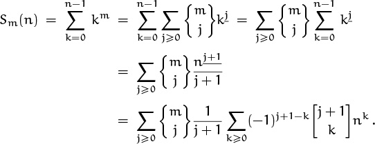
The next important sequence of numbers on our agenda is named after Jakob Bernoulli (1654–1705), who discovered curious relationships while working out the formulas for sums of mth powers [26]. Let’s write

(Thus, when m > 0 we have in the notation of generalized harmonic numbers.) Bernoulli looked at the following sequence of formulas and spotted a pattern:

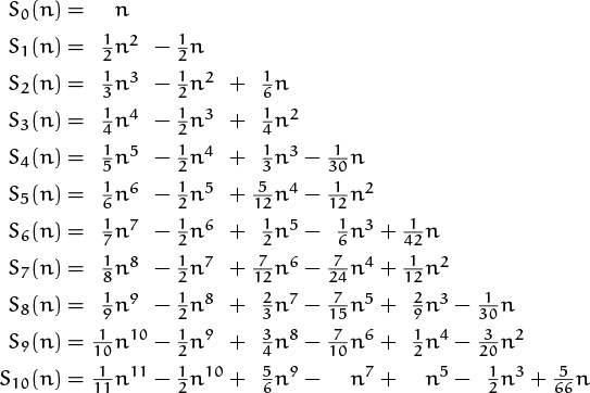
Can you see it too? The coefficient of n^m+1 in S_m(n) is always 1/(m + 1). The coefficient of n^m is always –1/2. The coefficient of n^m–1 is always . . . let’s see . . . m/12. The coefficient of n^m–2 is always zero. The coefficient of n^m–3 is always . . . let’s see . . . hmmm . . . yes, it’s –m(m–1)(m–2)/720. The coefficient of n^m–4 is always zero. And it looks as if the pattern will continue, with the coefficient of n^m–k always being some constant times m^k.

That was Bernoulli’s empirical discovery. (He did not give a proof.) In modern notation we write the coefficients in the form

Bernoulli numbers are defined by an implicit recurrence relation,

For example, . The first few values turn out to be

(All conjectures about a simple closed form for B_n are wiped out by the appearance of the strange fraction –691/2730.)

We can prove Bernoulli’s formula (6.78) by induction on m, using the perturbation method (one of the ways we found S₂(n) = _n in Chapter 2):

Let Ŝ_m(n) be the right-hand side of (6.78); we wish to show that S_m(n) = Ŝ_m(n), assuming that S_j(n) = Ŝ_j(n) for 0 ≤ j < m. We begin as we did for m = 2 in Chapter 2, subtracting S_m+1(n) from both sides of (6.80). Then we expand each S_j(n) using (6.78), and regroup so that the coefficients of powers of n on the right-hand side are brought together and simplified:

(This derivation is a good review of the standard manipulations we learned in Chapter 5.) Thus Δ = 0 and S_m(n) = Ŝ_m(n), QED.

In Chapter 7 we’ll use generating functions to obtain a much simpler proof of (6.78). The key idea will be to show that the Bernoulli numbers are the coefficients of the power series

Here’s some more neat stuff that you’ll probably want to skim through the first time.

—Friendly TA

Let’s simply assume for now that equation (6.81) holds, so that we can derive some of its amazing consequences. If we add z to both sides, thereby cancelling the term B₁z/1! = – z from the right, we get

Here coth is the “hyperbolic cotangent” function, otherwise known in calculus books as cosh z/sinh z; we have

Changing z to –z gives coth coth ; hence every odd-numbered coefficient of coth must be zero, and we have

Furthermore (6.82) leads to a closed form for the coefficients of coth:

But there isn’t much of a market for hyperbolic functions; people are more interested in the “real” functions of trigonometry. We can express ordinary trigonometric functions in terms of their hyperbolic cousins by using the rules

the corresponding power series are

Hence cot z = cos z/sin z = i cosh iz/ sinh iz = i coth iz, and we have

I see, we get “real” functions by using imaginary numbers.

Another remarkable formula for z cot z was found by Euler (exercise 73):

We can expand Euler’s formula in powers of z², obtaining

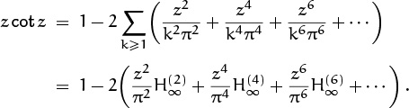
Equating coefficients of z²ⁿ with those in our other formula, (6.87), gives us an almost miraculous closed form for infinitely many infinite sums:

For example,

Formula (6.89) is not only a closed form for , it also tells us the approximate size of B_2n, since is very near 1 when n is large. And it tells us that (–1)^n–1B_2n > 0 for all n > 0; thus the nonzero Bernoulli numbers alternate in sign.

And that’s not all. Bernoulli numbers also appear in the coefficients of the tangent function,

as well as other trigonometric functions (exercise 72). Formula (6.92) leads to another important fact about the Bernoulli numbers, namely that

We have, for example:

(The T’s are called tangent numbers.)

One way to prove (6.93), following an idea of B. F. Logan, is to consider the power series

where T_n(x) is a polynomial in x; setting x = 0 gives T_n(0) = T_n, the nth tangent number. If we differentiate (6.94) with respect to x, we get

When x = tan w, this is tan(z + w). Hence, by Taylor’s theorem, the nth derivative of tan w is T_n(tan w).

but if we differentiate with respect to z, we get

(Try it—the cancellation is very pretty.) Therefore we have

a simple recurrence from which it follows that the coefficients of T_n(x) are nonnegative integers. Moreover, we can easily prove that T_n(x) has degree n + 1, and that its coefficients are alternately zero and positive. Therefore T_2n+1(0) = T_2n+1 is a positive integer, as claimed in (6.93).

Recurrence (6.95) gives us a simple way to calculate Bernoulli numbers, via tangent numbers, using only simple operations on integers; by contrast, the defining recurrence (6.79) involves difficult arithmetic with fractions.

If we want to compute the sum of mth powers from a to b – 1 instead of from 0 to n – 1, the theory of Chapter 2 tells us that

This identity has interesting consequences when we consider negative values of k: We have

hence

S_m(0) – S_m(–n + 1) = (–1)^m (S_m(n) – S_m(0)).

But S_m(0) = 0, so we have the identity

Therefore S_m(1) = 0. If we write the polynomial S_m(n) in factored form, it will always have the factors n and (n –1), because it has the roots 0 and 1. In general, S_m(n) is a polynomial of degree m + 1 with leading term . Moreover, we can set in (6.97) to deduce that ; if m is even, this makes , so will be an additional factor. These observations explain why we found the simple factorization

(Johann Faulhaber implicitly used (6.97) in 1631 [119] to find simple formulas for S_m(n) as polynomials in n(n + 1)/2 when m ≤ 17; see [222].)

in Chapter 2; we could have used such reasoning to deduce the value of S₂(n) without calculating it! Furthermore, (6.97) implies that the polynomial with the remaining factors, Ŝ_m(n) = S_m(n)/, always satisfies

Ŝ_m(1 – n) = Ŝ_m(n),          m even,     m > 0.

It follows that S_m(n) can always be written in the factored form

Here , and α₂, . . . , α_m/2 are appropriate complex numbers whose values depend on m. For example,

If m is odd and greater than 1, we have B_m = 0; hence S_m(n) is divisible by n² (and by (n – 1)²). Otherwise the roots of S_m(n) don’t seem to obey a simple law.

Let’s conclude our study of Bernoulli numbers by looking at how they relate to Stirling numbers. One way to compute S_m(n) is to change ordinary powers to falling powers, since the falling powers have easy sums. After doing those easy sums we can convert back to ordinary powers:

Therefore, equating coefficients with those in (6.78), we must have the identity

It would be nice to prove this relation directly, thereby discovering Bernoulli numbers in a new way. But the identities in Tables 264 or 265 don’t give us any obvious handle on a proof by induction that the left-hand sum in (6.99) is a constant times m^k–1. If k = m + 1, the left-hand sum is just , so that case is easy. And if k = m, the left-hand side sums to ; so that case is pretty easy too. But if k < m, the left-hand sum looks hairy. Bernoulli would probably not have discovered his numbers if he had taken this route.

One thing we can do is replace by . The (j + 1) nicely cancels with the awkward denominator, and the left-hand side becomes

The second sum is zero, when k < m, by (6.31). That leaves us with the first sum, which cries out for a change in notation; let’s rename all variables so that the index of summation is k, and so that the other parameters are m and n. Then identity (6.99) is equivalent to

Good, we have something that looks more pleasant—although Table 265 still doesn’t suggest any obvious next step.

The convolution formulas in Table 272 now come to the rescue. We can use (6.49) and (6.48) to rewrite the summand in terms of Stirling polynomials:

Things are looking up; the convolution in (6.46), with t = 1, yields

Formula (6.100) is now verified, and we find that Bernoulli numbers are related to the constant terms in the Stirling polynomials:

6.6 Fibonacci Numbers

Now we come to a special sequence of numbers that is perhaps the most pleasant of all, the Fibonacci sequence F_n:

Unlike the harmonic numbers and the Bernoulli numbers, the Fibonacci numbers are nice simple integers. They are defined by the recurrence

The simplicity of this rule—the simplest possible recurrence in which each number depends on the previous two—accounts for the fact that Fibonacci numbers occur in a wide variety of situations.

“Bee trees” provide a good example of how Fibonacci numbers can arise naturally. Let’s consider the pedigree of a male bee. Each male (also known as a drone) is produced asexually from a female (also known as a queen); each female, however, has two parents, a male and a female. Here are the first few levels of the tree:

The back-to-nature nature of this example is shocking. This book should be banned.

The drone has one grandfather and one grandmother; he has one greatgrandfather and two great-grandmothers; he has two great-great-grandfathers and three great-great-grandmothers. In general, it is easy to see by induction that he has exactly F_n+1 greatⁿ-grandpas and F_n+2 greatⁿ-grandmas.

Fibonacci numbers are often found in nature, perhaps for reasons similar to the bee-tree law. For example, a typical sunflower has a large head that contains spirals of tightly packed florets, usually with 34 winding in one direction and 55 in another. Smaller heads will have 21 and 34, or 13 and 21; a gigantic sunflower with 89 and 144 spirals was once exhibited in England. Similar patterns are found in some species of pine cones.

Phyllotaxis, n. The love of taxis.

And here’s an example of a different nature [277]: Suppose we put two panes of glass back-to-back. How many ways a_n are there for light rays to pass through or be reflected after changing direction n times? The first few cases are:

When n is even, we have an even number of bounces and the ray passes through; when n is odd, the ray is reflected and it re-emerges on the same side it entered. The a_n’s seem to be Fibonacci numbers, and a little staring at the figure tells us why: For n ≥ 2, the n-bounce rays either take their first bounce off the opposite surface and continue in a_n–1 ways, or they begin by bouncing off the middle surface and then bouncing back again to finish in a_n–2 ways. Thus we have the Fibonacci recurrence a_n = a_n–1 + a_n–2. The initial conditions are different, but not very different, because we have a₀ = 1 = F₂ and a₁ = 2 = F₃; therefore everything is simply shifted two places, and a_n = F_n+2.

Leonardo Fibonacci introduced these numbers in 1202, and mathematicians gradually began to discover more and more interesting things about them. Edouard Lucas, the perpetrator of the Tower of Hanoi puzzle discussed in Chapter 1, worked with them extensively in the last half of the nineteenth century (in fact it was Lucas who popularized the name “Fibonacci numbers”). One of his amazing results was to use properties of Fibonacci numbers to prove that the 39-digit Mersenne number 2¹²⁷ – 1 is prime.

“La suite de Fibonacci possède des propriétés nombreuses fort intéressantes.”

—E. Lucas [259]

One of the oldest theorems about Fibonacci numbers, first published by the Italian astronomer Gian Domenico Cassini in 1680 [51], is the identity

When n = 6, for example, Cassini’s identity correctly claims that 13·5 – 8² equals 1. (Johannes Kepler knew this law already in 1608 [202].)

A polynomial formula that involves Fibonacci numbers of the form F_n±k for small values of k can be transformed into a formula that involves only F_n and F_n+1, because we can use the rule

to express F_m in terms of higher Fibonacci numbers when m < n, and we can use

to replace F_m by lower Fibonacci numbers when m > n+1. Thus, for example, we can replace F_n–1 by F_n+1 – F_n in (6.103) to get Cassini’s identity in the form

Moreover, Cassini’s identity reads

F_n+2 F_n – = (–1)ⁿ⁺¹

when n is replaced by n + 1; this is the same as (F_n+1 + F_n)F_n – = (–1)ⁿ⁺¹, which is the same as (6.106). Thus Cassini(n) is true if and only if Cassini(n+1) is true; equation (6.103) holds for all n by induction.

Cassini’s identity is the basis of a geometrical paradox that was one of Lewis Carroll’s favorite puzzles [63], [319], [364]. The idea is to take a chessboard and cut it into four pieces as shown here, then to reassemble the pieces into a rectangle:

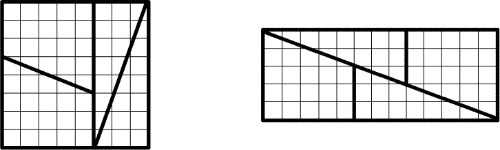
Presto: The original area of 8 × 8 = 64 squares has been rearranged to yield 5 × 13 = 65 squares! A similar construction dissects any F_n × F_n square into four pieces, using F_n+1, F_n, F_n–1, and F_n–2 as dimensions wherever the illustration has 13, 8, 5, and 3 respectively. The result is an F_n–1 × F_n+1 rectangle; by (6.103), one square has therefore been gained or lost, depending on whether n is even or odd.

The paradox is explained because . . . well, magic tricks aren’t supposed to be explained.

Strictly speaking, we can’t apply the reduction (6.105) unless m ≥ 2, because we haven’t defined F_n for negative n. A lot of maneuvering becomes easier if we eliminate this boundary condition and use (6.104) and (6.105) to define Fibonacci numbers with negative indices. For example, F_–1 turns out to be F₁ – F₀ = 1; then F_–2 is F₀ – F_–1 = –1. In this way we deduce the values

and it quickly becomes clear (by induction) that

Cassini’s identity (6.103) is true for all integers n, not just for n > 0, when we extend the Fibonacci sequence in this way.

The process of reducing F_n±k to a combination of F_n and F_n+1 by using (6.105) and (6.104) leads to the sequence of formulas

Fn+2    =      Fn+1 +   Fn		Fn–1   =     Fn+1   –     Fn
Fn+3    =    2Fn+1 +   Fn		Fn–2   =   –Fn+1   +  2Fn
Fn+4    =    3Fn+1 + 2Fn		Fn–3   =     2Fn+1  –  3Fn
Fn+5    =    5Fn+1 + 3Fn		Fn–4   =   –3Fn+1  +  5Fn

in which another pattern becomes obvious:

This identity, easily proved by induction, holds for all integers k and n (positive, negative, or zero).

If we set k = n in (6.108), we find that

hence F_2n is a multiple of F_n. Similarly,

F_3n = F_2nF_n+1 + F_2n–1F_n ,

and we may conclude that F_3n is also a multiple of F_n. By induction,

for all integers k and n. This explains, for example, why F₁₅ (which equals 610) is a multiple of both F₃ and F₅ (which are equal to 2 and 5). Even more is true, in fact; exercise 27 proves that

For example, gcd(F₁₂, F₁₈) = gcd(144, 2584) = 8 = F₆.

We can now prove a converse of (6.110): If n > 2 and if F_m is a multiple of F_n, then m is a multiple of n. For if F_nF_m then F_ngcd(F_m, F_n) = F_gcd(m,n) ≤ F_n. This is possible only if F_gcd(m,n) = F_n; and our assumption that n > 2 makes it mandatory that gcd(m, n) = n. Hence nm.

An extension of these divisibility ideas was used by Yuri Matijasevich in his famous proof [266] that there is no algorithm to decide if a given multivariate polynomial equation with integer coefficients has a solution in integers. Matijasevich’s lemma states that, if n > 2, the Fibonacci number F_m is a multiple of if and only if m is a multiple of nF_n.

Let’s prove this by looking at the sequence F_kn mod for k = 1, 2, 3, . . . , and seeing when F_kn mod = 0. (We know that m must have the form kn if F_m mod F_n = 0.) First we have F_n mod = F_n; that’s not zero. Next we have

F_2n = F_nF_n+1 + F_n–1F_n ≡ 2F_nF_n+1          (mod ),

by (6.108), since F_n+1 ≡ F_n–1 (mod F_n). Similarly

This congruence allows us to compute

F3n	= F2n+1Fn + F2nFn–1
	≡ Fn + (2FnFn+1)Fn+1 = 3Fn          (mod );
F3n+1	= F2n+1Fn+1 + F2nFn
	≡ + (2FnFn+1)Fn ≡                           (mod ) .

In general, we find by induction on k that

Now F_n+1 is relatively prime to F_n, so

Fkn ≡ 0 (mod )		kFn ≡ 0 (mod )
		k ≡ 0 (mod Fn) .

We have proved Matijasevich’s lemma.

One of the most important properties of the Fibonacci numbers is the special way in which they can be used to represent integers. Let’s write

Then every positive integer has a unique representation of the form

[The anonymous author of a classic Sanskrit work, Prākṛta Paiṅgala (c. 1320), actually knew this representation many centuries ago.]

(This is “Zeckendorf’s theorem” [246], [381].) For example, the representation of one million turns out to be

1000000	= 832040 + 121393 + 46368 + 144 + 55
	=    F30     +    F26     +    F24   +  F12 + F10 .

We can always find such a representation by using a “greedy” approach, choosing F_k1 to be the largest Fibonacci number ≤ n, then choosing F_k2 to be the largest that is ≤ n – F_k1, and so on. (More precisely, suppose that F_k ≤ n < F_k+1; then we have 0 ≤ n – F_k < F_k+1 – F_k = F_k–1. If n is a Fibonacci number, (6.113) holds with r = 1 and k₁ = k. Otherwise n – F_k has a Fibonacci representation F_k2 + · · · + F_kr, by induction on n; and (6.113) holds if we set k₁ = k, because the inequalities F_k2 ≤ n – F_k < F_k–1 imply that k ≫ k₂.) Conversely, any representation of the form (6.113) implies that

F_k1 ≤ n < F_k1+1 ,

because the largest possible value of F_k2 + · · · + F_kr when k ≫ k₂ ≫ · · · ≫ k_r ≫ 0 is

(This formula is easy to prove by induction on k; the left-hand side is zero when k is 2 or 3.) Therefore k₁ is the greedily chosen value described earlier, and the representation must be unique.

Any system of unique representation is a number system; therefore Zeckendorf’s theorem leads to the Fibonacci number system. We can represent any nonnegative integer n as a sequence of 0’s and 1’s, writing

This number system is something like binary (radix 2) notation, except that there never are two adjacent 1’s. For example, here are the numbers from 1 to 20, expressed Fibonacci-wise:

1 = (000001)F	6 = (001001)F	11 = (010100)F	16 = (100100)F
2 = (000010)F	7 = (001010)F	12 = (010101)F	17 = (100101)F
3 = (000100)F	8 = (010000)F	13 = (100000)F	18 = (101000)F
4 = (000101)F	9 = (010001)F	14 = (100001)F	19 = (101001)F
5 = (001000)F	10 = (010010)F	15 = (100010)F	20 = (101010)F

The Fibonacci representation of a million, shown a minute ago, can be contrasted with its binary representation 2¹⁹ + 2¹⁸ + 2¹⁷ + 2¹⁶ + 2¹⁴ + 2⁹ + 2⁶:

(1000000)₁₀ = (10001010000000000010100000000)_F

       = (11110100001001000000)₂ .

The Fibonacci representation needs a few more bits because adjacent 1’s are not permitted; but the two representations are analogous.

To add 1 in the Fibonacci number system, there are two cases: If the “units digit” is 0, we change it to 1; that adds F₂ = 1, since the units digit refers to F₂. Otherwise the two least significant digits will be 01, and we change them to 10 (thereby adding F₃ – F₂ = 1). Finally, we must “carry” as much as necessary by changing the digit pattern ‘011’ to ‘100’ until there are no two 1’s in a row. (This carry rule is equivalent to replacing F_m+1 + F_m by F_m+2.) For example, to go from 5 = (1000)_F to 6 = (1001)_F or from 6 = (1001)_F to 7 = (1010)_F requires no carrying; but to go from 7 = (1010)_F to 8 = (10000)_F we must carry twice.

So far we’ve been discussing lots of properties of the Fibonacci numbers, but we haven’t come up with a closed formula for them. We haven’t found closed forms for Stirling numbers, Eulerian numbers, or Bernoulli numbers either; but we were able to discover the closed form for harmonic numbers. Is there a relation between F_n and other quantities we know? Can we “solve” the recurrence that defines F_n?

The answer is yes. In fact, there’s a simple way to solve the recurrence by using the idea of generating function that we looked at briefly in Chapter 5. Let’s consider the infinite series

If we can find a simple formula for F(z), chances are reasonably good that we can find a simple formula for its coefficients F_n.

“Sit 1 + x + 2xx + 3x³ + 5x⁴ + 8x⁵ + 13x⁶ + 21x⁷ + 34x⁸ &c Series nata ex divisione Unitatis per Trinomium 1 – x – xx.”

—A. de Moivre [76]

“The quantities r, s, t, which show the relation of the terms, are the same as those in the denominator of the fraction. This property, howsoever obvious it may be, M. DeMoivre was the first that applied it to use, in the solution of problems about infinite series, which otherwise would have been very intricate.”

—J. Stirling [343]

In Chapter 7 we will focus on generating functions in detail, but it will be helpful to have this example under our belts by the time we get there. The power series F(z) has a nice property if we look at what happens when we multiply it by z and by z²:

F(z) =	F0 + F1z + F2z2 + F3z3 + F4z4 + F5z5 + · · · ,
zF(z) =	F0z + F1z2 + F2z3 + F3z4 + F4z5 + · · · ,
z2F(z) =	F0z2 + F1z3 + F2z4 + F3z5 + · · · .

If we now subtract the last two equations from the first, the terms that involve z², z³, and higher powers of z will all disappear, because of the Fibonacci recurrence. Furthermore the constant term F₀ never actually appeared in the first place, because F₀ = 0. Therefore all that’s left after the subtraction is (F₁ – F₀)z, which is just z. In other words,

F(z) – zF(z) – z²F(z) = z ,

and solving for F(z) gives us the compact formula

We have now boiled down all the information in the Fibonacci sequence to a simple (although unrecognizable) expression z/(1 – z – z²). This, believe it or not, is progress, because we can factor the denominator and then use partial fractions to achieve a formula that we can easily expand in power series. The coefficients in this power series will be a closed form for the Fibonacci numbers.

The plan of attack just sketched can perhaps be understood better if we approach it backwards. If we have a simpler generating function, say 1/(1 – αz) where α is a constant, we know the coefficients of all powers of z, because

= 1 + αz + α²z² + α³z³ + · · · .

Similarly, if we have a generating function of the form A/(1–αz)+B/(1–βz), the coefficients are easily determined, because

Therefore all we have to do is find constants A, B, α, and β such that

and we will have found a closed form Aαⁿ + Bβⁿ for the coefficient F_n of zⁿ in F(z). The left-hand side can be rewritten

so the four constants we seek are the solutions to two polynomial equations:

We want to factor the denominator of F(z) into the form (1 – αz)(1 – βz); then we will be able to express F(z) as the sum of two fractions in which the factors (1 – αz) and (1 – βz) are conveniently separated from each other.

Notice that the denominator factors in (6.119) have been written in the form (1 – αz)(1 – βz), instead of the more usual form c(z – ρ₁)(z – ρ₂) where ρ₁ and ρ₂ are the roots. The reason is that (1 – αz)(1 – βz) leads to nicer expansions in power series.

We can find α and β in several ways, one of which uses a slick trick: Let us introduce a new variable w and try to find the factorization

w² – wz – z² = (w – αz)(w – βz) .

As usual, the authors can’t resist a trick.

Then we can simply set w = 1 and we’ll have the factors of 1 – z – z². The roots of w² – wz – z² = 0 can be found by the quadratic formula; they are

Therefore

and we have the constants α and β we were looking for.

The number is important in many parts of mathematics as well as in the art world, where it has been considered since ancient times to be the most pleasing ratio for many kinds of design. Therefore it has a special name, the golden ratio. We denote it by the Greek letter ϕ, in honor of Phidias who is said to have used it consciously in his sculpture. The other root shares many properties of ϕ, so it has the special name , “phi hat.” These numbers are roots of the equation w² – w – 1 = 0, so we have

The ratio of one’s height to the height of one’s navel is approximately 1.618, according to extensive empirical observations by European scholars [136].

(More about ϕ and later.)

We have found the constants α = ϕ and needed in (6.119); now we merely need to find A and B in (6.120). Setting z = 0 in that equation tells us that B = –A, so (6.120) boils down to

The solution is ; the partial fraction expansion of (6.117) is therefore

Good, we’ve got F(z) right where we want it. Expanding the fractions into power series as in (6.118) gives a closed form for the coefficient of zⁿ:

(This formula was first published by Daniel Bernoulli in 1728, but people forgot about it until it was rediscovered by Jacques Binet [31] in 1843.)

Before we stop to marvel at our derivation, we should check its accuracy. For n = 0 the formula correctly gives F₀ = 0; for n = 1, it gives , which is indeed 1. For higher powers, equations (6.121) show that the numbers defined by (6.123) satisfy the Fibonacci recurrence, so they must be the Fibonacci numbers by induction. (We could also expand ϕⁿ and by the binomial theorem and chase down the various powers of ; but that gets pretty messy. The point of a closed form is not necessarily to provide us with a fast method of calculation, but rather to tell us how F_n relates to other quantities in mathematics.)

With a little clairvoyance we could simply have guessed formula (6.123) and proved it by induction. But the method of generating functions is a powerful way to discover it; in Chapter 7 we’ll see that the same method leads us to the solution of recurrences that are considerably more difficult. Incidentally, we never worried about whether the infinite sums in our derivation of (6.123) were convergent; it turns out that most operations on the coefficients of power series can be justified rigorously whether or not the sums actually converge [182]. Still, skeptical readers who suspect fallacious reasoning with infinite sums can take comfort in the fact that equation (6.123), once found by using infinite series, can be verified by a solid induction proof.

One of the interesting consequences of (6.123) is that the integer F_n is extremely close to the irrational number when n is large. (Since is less than 1 in absolute value, becomes exponentially small and its effect is almost negligible.) For example, F₁₀ = 55 and F₁₁ = 89 are very near

We can use this observation to derive another closed form,

because for all n ≥ 0. When n is even, F_n is a little bit less than ; otherwise it is a little greater.

Cassini’s identity (6.103) can be rewritten

When n is large, 1/F_n–1F_n is very small, so F_n+1/F_n must be very nearly the same as F_n/F_n–1; and (6.124) tells us that this ratio approaches ϕ. In fact, we have

(This identity is true by inspection when n = 0 or n = 1, and by induction when n > 1; we can also prove it directly by plugging in (6.123).) The ratio F_n+1/F_n is very close to ϕ, which it alternately overshoots and undershoots.

By coincidence, ϕ is also very nearly the number of kilometers in a mile. (The exact number is 1.609344, since 1 inch is exactly 2.54 centimeters.) This gives us a handy way to convert mentally between kilometers and miles, because a distance of F_n+1 kilometers is (very nearly) a distance of F_n miles.

Suppose we want to convert a non-Fibonacci number from kilometers to miles; what is 30 km, American style? Easy: We just use the Fibonacci number system and mentally convert 30 to its Fibonacci representation 21 + 8 + 1 by the greedy approach explained earlier. Now we can shift each number down one notch, getting 13 + 5 + 1. (The former ‘1’ was F₂, since k_r ≫ 0 in (6.113); the new ‘1’ is F₁.) Shifting down divides by ϕ, more or less. Hence 19 miles is our estimate. (That’s pretty close; the correct answer is about 18.64 miles.) Similarly, to go from miles to kilometers we can shift up a notch; 30 miles is approximately 34 + 13 + 2 = 49 kilometers. (That’s not quite as close; the correct number is about 48.28.)

If the USA ever goes metric, our speed limit signs will go from 55 mi/hr to 89 km/hr. Or maybe the highway people will be generous and let us go 90.

It turns out that this shift-down rule gives the correctly rounded number of miles per n kilometers for all n ≤ 100, except in the cases n = 4, 12, 54, 62, 75, 83, 91, 96, and 99, when it is off by less than 2/3 mile. And the shift-up rule gives either the correctly rounded number of kilometers for n miles, or 1 km too many, for all n ≤ 113. (The only really embarrassing case is n = 4, where the individual rounding errors for n = 3 + 1 both go the same direction instead of cancelling each other out.)

The “shift down” rule changes n to f(n/ϕ) and the “shift up” rule changes n to f(nϕ), where f(x) = x + ϕ^–1 .

6.7 Continuants

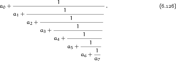
Fibonacci numbers have important connections to the Stern–Brocot tree that we studied in Chapter 4, and they have important generalizations to a sequence of polynomials that Euler studied extensively. These polynomials are called continuants, because they are the key to the study of continued fractions like

The continuant polynomial K_n(x₁, x₂, . . . , x_n) has n parameters, and it is defined by the following recurrence:

For example, the next three cases after K₁(x₁) are

K2(x1, x2)	=	x1x2 + 1 ;
K3(x1, x2, x3)	=	x1x2x3 + x1 + x3 ;
K4(x1, x2, x3, x4)	=	x1x2x3x4 + x1x2 + x1x4 + x3x4 + 1 .

It’s easy to see, inductively, that the number of terms is a Fibonacci number:

When the number of parameters is implied by the context, we can write simply ‘K’ instead of ‘K_n’, just as we can omit the number of parameters when we use the hypergeometric functions F of Chapter 5. For example, K(x₁, x₂) = K₂(x₁, x₂) = x₁x₂ + 1. The subscript n is of course necessary in formulas like (6.128).

Euler [112] observed that K(x₁, x₂, . . . , x_n) can be obtained by starting with the product x₁x₂ . . . x_n and then striking out adjacent pairs x_kx_k+1 in all possible ways. We can represent Euler’s rule graphically by constructing all “Morse code” sequences of dots and dashes having length n, where each dot contributes 1 to the length and each dash contributes 2; here are the Morse code sequences of length 4:

These dot-dash patterns correspond to the terms of K(x₁, x₂, x₃, x₄); a dot signifies a variable that’s included and a dash signifies a pair of variables that’s excluded. For example, corresponds to x₁x₄.

A Morse code sequence of length n that has k dashes has n – 2k dots and n – k symbols altogether. These dots and dashes can be arranged in ways; therefore if we replace each dot by z and each dash by 1 we get

We also know that the total number of terms in a continuant is a Fibonacci number; hence we have the identity

(A closed form for (6.129), generalizing the Euler–Binet formula (6.123) for Fibonacci numbers, appears in (5.74).)

The relation between continuant polynomials and Morse code sequences shows that continuants have a mirror symmetry:

Therefore they obey a recurrence that adjusts parameters at the left, in addition to the right-adjusting recurrence in definition (6.127):

Both of these recurrences are special cases of a more general law:

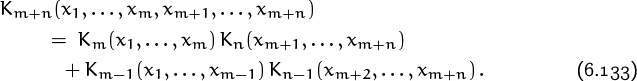
This law is easily understood from the Morse code analogy: The first product K_mK_n yields the terms of K_m+n in which there is no dash in the [m, m + 1] position, while the second product yields the terms in which there is a dash there. If we set all the x’s equal to 1, this identity tells us that F_m+n+1 = F_m+1F_n+1 + F_mF_n; thus, (6.108) is a special case of (6.133).

Euler [112] discovered that continuants obey an even more remarkable law, which generalizes Cassini’s identity:

This law (proved in exercise 29) holds whenever the subscripts on the K’s are all nonnegative. For example, when k = 2, m = 1, and n = 3, we have

K(x₁, x₂, x₃, x₄) K(x₂, x₃) = K(x₁, x₂, x₃) K(x₂, x₃, x₄) + 1 .

Continuant polynomials are intimately connected with Euclid’s algorithm. Suppose, for example, that the computation of gcd(m, n) finishes in four steps:

gcd(m, n) = gcd(n0, n1)		n0 = m ,         n1 = n ;
	= gcd(n1, n2)	n2 = n0 mod n1 = n0 – q1n1 ;
	= gcd(n2, n3)	n3 = n1 mod n2 = n1 – q2n2 ;
	= gcd(n3, n4)	n4 = n2 mod n3 = n2 – q3n3 ;
	= gcd(n4, 0) = n4 .	0 = n3 mod n4 = n3 – q4n4 .

Then we have

n4  =  n4	=  K()n4 ;
n3  =  q4n4	=  K(q4)n4 ;
n2  =  q3n3 + n4	=  K(q3, q4)n4 ;
n1  =  q2n2 + n3	=  K(q2, q3, q4)n4 ;
n0  =  q1n1 + n2	=  K(q1, q2, q3, q4)n4 .

In general, if Euclid’s algorithm finds the greatest common divisor d in k steps, after computing the sequence of quotients q₁, . . . , q_k, then the starting numbers were K(q₁, q₂, . . . , q_k)d and K(q₂, . . . , q_k)d. (This fact was noticed early in the eighteenth century by Thomas Fantet de Lagny [232], who seems to have been the first person to consider continuants explicitly. Lagny pointed out that consecutive Fibonacci numbers, which occur as continuants when the q’s take their minimum values, are therefore the smallest inputs that cause Euclid’s algorithm to take a given number of steps.)

Continuants are also intimately connected with continued fractions, from which they get their name. We have, for example,

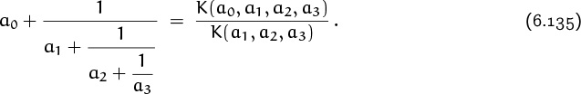
The same pattern holds for continued fractions of any depth. It is easily proved by induction; we have, for example,

because of the identity

(This identity is proved and generalized in exercise 30.)

Moreover, continuants are closely connected with the Stern–Brocot tree discussed in Chapter 4. Each node in that tree can be represented as a sequence of L’s and R’s, say

where a₀ ≥ 0, a₁ ≥ 1, a₂ ≥ 1, a₃ ≥ 1, . . . , a_n–2 ≥ 1, a_n–1 ≥ 0, and n is even. Using the 2 × 2 matrices L and R of (4.33), it is not hard to prove by induction that the matrix equivalent of (6.137) is

(The proof is part of exercise 87.) For example,

Finally, therefore, we can use (4.34) to write a closed form for the fraction in the Stern–Brocot tree whose L-and-R representation is (6.137):

(This is “Halphen’s theorem” [174].) For example, to find the fraction for LRRL we have a₀ = 0, a₁ = 1, a₂ = 2, a₃ = 1, and n = 4; equation (6.139) gives

(We have used the rule K_n(x₁, . . . , x_n–1, x_n + 1) = K_n+1(x₁, . . . , x_n–1, x_n, 1) to absorb leading and trailing 1’s in the parameter lists; this rule is obtained by setting y = 1 in (6.136).)

A comparison of (6.135) and (6.139) shows that the fraction corresponding to a general node (6.137) in the Stern–Brocot tree has the continued fraction representation

Thus we can convert at sight between continued fractions and the corresponding nodes in the Stern–Brocot tree. For example,

We observed in Chapter 4 that irrational numbers define infinite paths in the Stern–Brocot tree, and that they can be represented as an infinite string of L’s and R’s. If the infinite string for α is R^a₀ L^a₁ R^a₂ L^a₃ . . . , there is a corresponding infinite continued fraction

This infinite continued fraction can also be obtained directly: Let α₀ = α and for k ≥ 0 let

The a’s are called the “partial quotients” of α. If α is rational, say m/n, this process runs through the quotients found by Euclid’s algorithm and then stops (with α_k+1 = ∞).

Is Euler’s constant γ rational or irrational? Nobody knows. We can get partial information about this famous unsolved problem by looking for γ in the Stern–Brocot tree; if it’s rational we will find it, and if it’s irrational we will find all the closest rational approximations to it. The continued fraction for γ begins with the following partial quotients:

Or if they do, they’re not talking.

Therefore its Stern–Brocot representation begins LRLLRLLRLLLLRRRL . . . ; no pattern is evident. Calculations by Richard Brent [38] have shown that, if γ is rational, its denominator must be more than 10,000 decimal digits long. Therefore nobody believes that γ is rational; but nobody so far has been able to prove that it isn’t.

Well, γ must be irrational, because of a little-known Einsteinian assertion: “God does not throw huge denominators at the universe.”

Let’s conclude this chapter by proving a remarkable identity that ties a lot of these ideas together. We introduced the notion of spectrum in Chapter 3; the spectrum of α is the multiset of numbers nα, where α is a given constant. The infinite series

can therefore be said to be the generating function for the spectrum of ϕ, where is the golden ratio. The identity we will prove, discovered in 1976 by J. L. Davison [73], uses an infinite continued fraction to connect this generating function with the Fibonacci sequence:

Both sides of (6.143) are interesting; let’s look first at the numbers nϕ. If the Fibonacci representation (6.113) of n is F_k1 + · · · + F_kr, we expect nϕ to be approximately F_k1+1 + · · · + F_kr+1, the number we get from shifting the Fibonacci representation left (as when converting from miles to kilometers). In fact, we know from (6.125) that

nϕ = F_k1+1 + · · · + F_kr+1 – (^k₁ + · · · + ^k_r) .

Now = –1/ϕ and k₁ ≫ · · · ≫ k_r ≫ 0, so we have

and ^k₁ + · · · + ^k_r has the same sign as (–1)^k_r, by a similar argument. Hence

Let us say that a number n is Fibonacci odd (or F-odd for short) if its least significant Fibonacci bit is 1; this is the same as saying that k_r(n) = 2. Otherwise n is Fibonacci even (F-even). For example, the smallest F-odd numbers are 1, 4, 6, 9, 12, 14, 17, and 19. If k_r(n) is even, then n – 1 is F-even, by (6.114); similarly, if k_r(n) is odd, then n – 1 is F-odd. Therefore

k_r(n) is even                    n – 1 is F-even.

Furthermore, if k_r(n) is even, (6.144) implies that k_r (nϕ) = 2; if k_r(n) is odd, (6.144) says that k_r (nϕ) = k_r(n) + 1. Therefore k_r (nϕ) is always even, and we have proved that

nϕ – 1 is always F-even.

Conversely, if m is any F-even number, we can reverse this computation and find an n such that m + 1 = nϕ. (First add 1 in F-notation as explained earlier. If no carries occur, n is (m + 2) shifted right; otherwise n is (m + 1) shifted right.) The right-hand sum of (6.143) can therefore be written

How about the fraction on the left? Let’s rewrite (6.143) so that the continued fraction looks like (6.141), with all numerators 1:

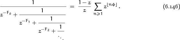
(This transformation is a bit tricky! The numerator and denominator of the original fraction having z^F_n as numerator should be divided by z^F_n–1.) If we stop this new continued fraction at 1/z^–F_n, its value will be a ratio of continuants,

as in (6.135). Let’s look at the denominator first, in hopes that it will be tractable. Setting Q_n = K_n+1(z^–F₀ , . . . , z^–F_n ), we find Q₀ = 1, Q₁ = 1+z^–1, Q₂ = 1+z^–1 +z^–2, Q₃ = 1+z^–1 +z^–2 +z^–3 +z^–4, and in general everything fits beautifully and gives a geometric series

Q_n = 1 + z^–1 + z^–2 + · · · + z^{–(F_n+2–1)} .

The corresponding numerator is P_n = K_n(z^–F₁ , . . . , z^–F_n ); this turns out to be like Q_n but with fewer terms. For example, we have

P₅ = z^–1 + z^–2 + z^–4 + z^–5 + z^–7 + z^–9 + z^–10 + z^–12 ,

compared with Q₅ = 1 + z^–1 + · · · + z^–12. A closer look reveals the pattern governing which terms are present: We have

and in general we can prove by induction that

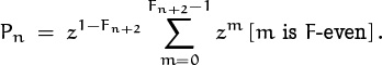
Therefore

Taking the limit as n → ∞ now gives (6.146), because of (6.145).

Exercises

Warmups

1. What are the permutations of {1, 2, 3, 4} that have exactly two cycles? (The cyclic forms appear in (6.4); non-cyclic forms like 2314 are desired instead.)

2. There are mⁿ functions from a set of n elements into a set of m elements. How many of them range over exactly k different function values?

3. Card stackers in the real world know that it’s wise to allow a bit of slack so that the cards will not topple over when a breath of wind comes along. Suppose the center of gravity of the top k cards is required to be at least units from the edge of the k + 1st card. (Thus, for example, the first card can overhang the second by at most 1– units.) Can we still achieve arbitrarily large overhang, if we have enough cards?

4. Express 1/1 + 1/3 + · · · + 1/(2n+1) in terms of harmonic numbers.

5. Explain how to get the recurrence (6.75) from the definition of U_n(x, y) in (6.74), and solve the recurrence.

6. An explorer has left a pair of baby rabbits on an island. If baby rabbits become adults after one month, and if each pair of adult rabbits produces one pair of baby rabbits every month, how many pairs of rabbits are present after n months? (After two months there are two pairs, one of which is newborn.) Find a connection between this problem and the “bee tree” in the text.

If the harmonic numbers are worm numbers, the Fibonacci numbers are rabbit numbers.

7. Show that Cassini’s identity (6.103) is a special case of (6.108), and a special case of (6.134).

8. Use the Fibonacci number system to convert 65 mi/hr into an approximate number of km/hr.

9. About how many square kilometers are in 8 square miles?

10. What is the continued fraction representation of ϕ?

Basics

11. What is , the row sum of Stirling’s cycle-number triangle with alternating signs, when n is a nonnegative integer?

12. Prove that Stirling numbers have an inversion law analogous to (5.48):

13. The differential operators and ϑ = zD are mentioned in Chapters 2 and 5. We have

ϑ² = z²D² + zD ,

because ϑ²f(z) = ϑzf′(z) = z zf′(z) = z²f″(z) + zf′(z), which is (z²D² +zD)f(z). Similarly it can be shown that ϑ³ = z³D³ +3z²D² +zD. Prove the general formulas

for all n ≥ 0. (These can be used to convert between differential expressions of the forms ∑_k α_kz^kf^(k)(z) and ∑_k β_kϑ^kf(z), as in (5.109).)

14. Prove the power identity (6.37) for Eulerian numbers.

15. Prove the Eulerian identity (6.39) by taking the mth difference of (6.37).

16. What is the general solution of the double recurrence

A_n,0 = a_n [n ≥ 0];          A_0,k = 0,          if k > 0;
A_n,k = kA_n–1,k + A_n–1,k–1 ,          integers k, n,

when k and n range over the set of all integers?

17. Solve the following recurrences, assuming that is zero when n < 0 or k < 0:

a.

b.

c.

18. Prove that the Stirling polynomials satisfy

(x + 1) σ_n(x + 1) = (x – n) σ_n(x) + xσ_n–1(x) .

19. Prove that the generalized Stirling numbers satisfy

20. Find a closed form for .

21. Show that if H_n = a_n/b_n where a_n and b_n are integers, the denominator b_n is a multiple of 2^{lg n}. Hint: Consider the number 2^{lg n–1}H_n – .

22. Prove that the infinite sum

converges for all complex numbers z, except when z is a negative integer; and show that it equals H_z when z is a nonnegative integer. (Therefore we can use this formula to define harmonic numbers H_z when z is complex.)

23. Equation (6.81) gives the coefficients of z/(e^z – 1), when expanded in powers of z. What are the coefficients of z/(e^z + 1)? Hint: Consider the identity (e^z + 1)(e^z – 1) = e^2z – 1.

24. Prove that the tangent number T_2n+1 is a multiple of 2ⁿ. Hint: Prove that all coefficients of T_2n(x) and T_2n+1(x) are multiples of 2ⁿ.

25. Equation (6.57) proves that the worm will eventually reach the end of the rubber band at some time N. Therefore there must come a first time n when he’s closer to the end after n minutes than he was after n – 1 minutes. Show that .

26. Use summation by parts to evaluate . Hint: Consider also the related sum .

27. Prove the gcd law (6.111) for Fibonacci numbers.

28. The Lucas number L_n is defined to be F_n+1 + F_n–1. Thus, according to (6.109), we have F_2n = F_nL_n. Here is a table of the first few values:

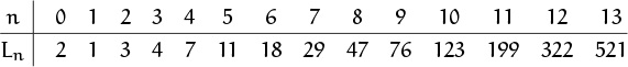
a. Use the repertoire method to show that the solution Q_n to the general recurrence

Q₀ = α ;      Q₁ = β ;      Q_n =  Q_n–1 + Q_n–2 ,      n > 1

can be expressed in terms of F_n and L_n.

b. Find a closed form for L_n in terms of ϕ and .

29. Prove Euler’s identity for continuants, equation (6.134).

30. Generalize (6.136) to find an expression for the incremented continuant K(x₁, . . . , x_m–1, x_m + y, x_m+1, . . . , x_n), when 1 ≤ m ≤ n.

Homework exercises

31. Find a closed form for the coefficients in the representation of rising powers by falling powers:

(For example, , hence .)

32. In Chapter 5 we obtained the formulas

by unfolding the recurrence in two ways. What identities appear when the analogous recurrence is unwound?

33. Table 264 gives the values of and . What are closed forms (not involving Stirling numbers) for the next cases, and ?

34. What are and , if the basic recursion relation (6.35) is assumed to hold for all integers k and n, and if for all k < 0?

35. Prove that, for every > 0, there exists an integer n > 1 (depending on ) such that H_n mod 1 < .

36. Is it possible to stack n bricks in such a way that the topmost brick is not above any point of the bottommost brick, yet a person who weighs the same as 100 bricks can balance on the middle of the top brick without toppling the pile?

37. Express in terms of harmonic numbers, assuming that m and n are positive integers. What is the limiting value as n → ∞?

38. Find the indefinite sum .

39. Express in terms of n and H_n.

40. Prove that 1979 divides the numerator of , and give a similar result for 1987. Hint: Use Gauss’s trick to obtain a sum of fractions whose numerators are 1979. See also exercise 4.

Ah! Those were prime years.

41. Evaluate the sum

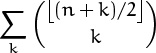
in closed form, when n is an integer (possibly negative).

42. If S is a set of integers, let S + 1 be the “shifted” set {x + 1 | x ∈ S}. How many subsets of {1, 2, . . . , n} have the property that S ∪ (S + 1) = {1, 2, . . . , n + 1}?

43. Prove that the infinite sum

   .1
+ .01
+ .002
+ .0003
+ .00005
+ .000008
+ .0000013
       .
       .
       .

converges to a rational number.

44. Prove the converse of Cassini’s identity (6.106): If k and m are integers such that |m²–km–k²| = 1, then there is an integer n such that k = ±F_n and m = ±F_n+1.

45. Use the repertoire method to solve the general recurrence

X₀ = α;     X₁ = β;      X_n = X_n–1 + X_n–2 + γn + δ .

46. What are cos 36° and cos 72°?

47. Show that

and use this identity to deduce the values of F_p mod p and F_p+1 mod p when p is prime.

48. Prove that zero-valued parameters can be removed from continuant polynomials by collapsing their neighbors together:

K_n(x₁, . . . , x_m–1, 0, x_m+1, . . . , x_n)

   = K_n–2(x₁, . . . , x_m–2, x_m–1+x_m+1, x_m+2, . . . , x_n) , 1 < m < n.

49. Find the continued fraction representation of the number ∑_n≥1 2^–nϕ.

50. Define f(n) for all positive integers n by the recurrence

f(1) = 1 ;

f(2n) = f(n) ;

f(2n + 1) = f(n) + f(n + 1) .

a. For which n is f(n) even?

b. Show that f(n) can be expressed in terms of continuants.

Exam problems

51. Let p be a prime number.

a. Prove that (mod p), for 1 < k < p.

b. Prove that , for 1 ≤ k < p.

c. Prove that , if p > 2.

d. Prove that if p > 3 we have . Hint: Consider .

52. Let H_n be written in lowest terms as a_n/b_n.

a. Prove that , if p is prime.

b. Find all n > 0 such that a_n is divisible by 5.

53. Find a closed form for , when 0 ≤ m ≤ n. Hint: Exercise 5.42 has the sum without the H_k factor.

54. Let n > 0. The purpose of this exercise is to show that the denominator of B_2n is the product of all primes p such that (p–1)(2n).

a. Show that S_m(p) + [(p–1)m] is a multiple of p, when p is prime and m > 0.

b. Use the result of part (a) to show that

Hint: It suffices to prove that, if p is any prime, the denominator of the fraction B_2n + [(p–1)(2n)]/p is not divisible by p.

c. Prove that the denominator of B_2n is always an odd multiple of 6, and it is equal to 6 for infinitely many n.

55. Prove (6.70) as a corollary of a more general identity, by summing

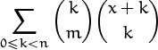
and differentiating with respect to x.

56. Evaluate in closed form as a function of the integers m and n. (The sum is over all integers k except for the value k = m.)

57. The “wraparound binomial coefficients of order 5” are defined by

and . Let Q_n be the difference between the largest and smallest of these numbers in row n:

Find and prove a relation between Q_n and the Fibonacci numbers.

58. Find closed forms for and . What do you deduce about the quantity ?

59. Prove that if m and n are positive integers, there exists an integer x such that F_x ≡ m (mod 3ⁿ).

60. Find all positive integers n such that either F_n + 1 or F_n – 1 is a prime number.

61. Prove the identity

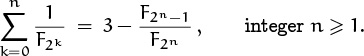
What is ?

62. Let A_n = ϕⁿ + ϕ^–n and B_n = ϕⁿ – ϕ^–n.

a. Find constants α and β such that A_n = αA_n–1 + βA_n–2 and B_n = αB_n–1 + βB_n–2 for all n ≥ 0.

b. Express A_n and B_n in terms of F_n and L_n (see exercise 28).

c. Prove that .

d. Find a closed form for .

Bogus problems

Bonus problems

63. How many permutations π₁π₂ . . . π_n of {1, 2, . . . , n} have exactly k indices j such that

a. π_i < π_j for all i < j? (Such j are called “left-to-right maxima.”)

b. π_j > j? (Such j are called “excedances.”)

64. What is the denominator of , when this fraction is reduced to lowest terms?

65. Prove the identity

66. What is , the nth alternating row sum of Euler’s triangle?

67. Prove that

68. Show that , and find a closed form for .

69. Find a closed form for .

70. Show that the complex harmonic numbers of exercise 22 have the power series expansion .

71. Prove that the generalized factorial of equation (5.83) can be written

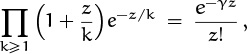
by considering the limit as n → ∞ of the first n factors of this infinite product. Show that is related to the general harmonic numbers of exercise 22.

72. Prove that the tangent function has the power series (6.92), and find the corresponding series for z/sin z and ln ((tan z)/z).

73. Prove that z cot z is equal to

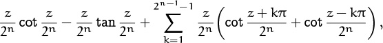
for all integers n ≥ 1, and show that the limit of the kth summand is 2z²/(z² – k²π²) for fixed k as n → ∞.

74. Find a relation between the numbers T_n(1) and the coefficients of 1/cos z.

75. Prove that the tangent numbers and the coefficients of 1/cos z appear at the edges of the infinite triangle that begins as follows:

1
0       1
1      1      0
0      1      2      2
5      5      4      2      0
0     5     10     14     16     16
61     61     56     46     32     16     0

Each row contains partial sums of the previous row, going alternately left-to-right and right-to-left. Hint: Consider the coefficients of the power series (sin z + cos z)/ cos(w + z).

76. Find a closed form for the sum

and show that it is zero when n is even.

77. When m and n are integers, n ≥ 0, the value of σ_n(m) is given by (6.48) if m < 0, by (6.49) if m > n, and by (6.101) if m = 0. Show that in the remaining cases we have

78. Prove the following relation that connects Stirling numbers, Bernoulli numbers, and Catalan numbers:

79. Show that the four chessboard pieces of the 64 = 65 paradox can also be reassembled to prove that 64 = 63.

80. A sequence defined by the recurrence A₁ = x, A₂ = y, and A_n = A_n–1 + A_n–2 has A_m = 1000000 for some m. What positive integers x and y make m as large as possible?

81. The text describes a way to change a formula involving F_n±k to a formula that involves F_n and F_n+1 only. Therefore it’s natural to wonder if two such “reduced” formulas can be equal when they aren’t identical in form. Let P(x, y) be a polynomial in x and y with integer coefficients. Find a necessary and sufficient condition that P(F_n+1, F_n) = 0 for all n ≥ 0.

82. Explain how to add positive integers, working entirely in the Fibonacci number system.

83. Is it possible that a sequence A_n satisfying the Fibonacci recurrence A_n = A_n–1 + A_n–2 can contain no prime numbers, if A₀ and A₁ are relatively prime?

84. Let m and n be odd, positive integers. Find closed forms for

Hint: The sums in exercise 62 are and .

85. Characterize all N such that the Fibonacci residues F_n mod N for n ≥ 0 form the complete set {0, 1, . . . , N – 1}. (See exercise 59.)

86. Let C₁, C₂, . . . be a sequence of nonzero integers such that

gcd(C_m, C_n) = C_gcd(m,n)

for all positive integers m and n. Prove that the generalized binomial coefficients

are all integers. (In particular, the “Fibonomial coefficients” formed in this way from Fibonacci numbers are integers, by (6.111).)

87. Show that continuant polynomials appear in the matrix product

and in the determinant

88. Generalizing (6.146), find a continued fraction related to the generating function ∑_n≥1 z^nα, when α is any positive irrational number.

89. Let α be an irrational number in (0 . . 1) and let a₁, a₂, a₃, . . . be the partial quotients in its continued fraction representation. Show that |D(α, n)| < 2 when n = K(a₁, . . . , a_m), where D is the discrepancy defined in Chapter 3.

90. Let Q_n be the largest denominator on level n of the Stern–Brocot tree. (Thus Q₀, Q₁, Q₂, Q₃, Q₄, . . . = 1, 2, 3, 5, 8, . . . according to the diagram in Chapter 4.) Prove that Q_n = F_n+2.

Research problems

91. What is the best way to extend the definition of to arbitrary real values of n and k?

92. Let H_n be written in lowest terms as a_n/b_n, as in exercise 52.

a. Are there infinitely many n with pa_n, for some fixed prime p?

b. Are there infinitely many n with b_n = lcm(1, 2, . . . , n)? (Two such values are n = 250 and n = 1000.)

93. Prove that γ and e^γ are irrational.

94. Develop a general theory of the solutions to the two-parameter recurrence

assuming that when n < 0 or k < 0. (Binomial coefficients, Stirling numbers, Eulerian numbers, and the sequences of exercises 17 and 31 are special cases.) What special values (α, β, γ, α′, β′, γ′) yield “fundamental solutions” in terms of which the general solution can be expressed?

95. Find an efficient way to extend the Gosper–Zeilberger algorithm from hypergeometric terms to terms that may involve Stirling numbers.