
Chapter 16
The time value of money and
net present value
A bird in the hand is worth two in the bush
For economic progress to be possible, there must be a universally applicable time value of money, even in a risk-free environment. This fundamental concept gives rise to the techniques of capitalisation, discounting and net present value, described below.
Section 16.1 Capitalisation
Consider an example of a businessman who invests €100 000 in his business at the end of 2007 and then sells it 10 years later for €1 800 000. In the meantime, he receives no income from his business, nor does he invest any additional funds into it. Here is a simple problem: given an initial outlay of €100 000 that becomes €1 800 000 in 10 years, and without any outside funds being invested in the business, what is the return on the businessman’s investment?
His profit after 10 years was €1 700 000 (€1 800 000 – €100 000) on an initial outlay of €100 000. Hence, his return was (1 700 000/100 000) or 1700% over a period of 10 years.
Is this a good result or not?
Actually, the return is not quite as impressive as it first looks. To find the annual return, our first thought might be to divide the total return (1700%) by the number of years (10) and say that the average return is 170% per year.
While this may look like a reasonable approach, it is in fact far from accurate. The value 170% has nothing to do with an annual return, which compares the funds invested and the funds recovered after one year. In the case above, there is no income for 10 years. Usually, calculating interest assumes a flow of revenue each year, which can then be reinvested, and which in turn begins producing additional interest.
There is only one sensible way to calculate the return on the above investment. First, it is necessary to seek the rate of return on a hypothetical investment that would generate income at the end of each year. After 10 years, the rate of return on the initial investment will have to have transformed €100 000 into €1 800 000. Further, the income generated must not be paid out, but rather it has to be reinvested (in which case the income is said to be capitalised).
Therefore, we are now trying to calculate the annual return on an investment that grows from €100 000 into €1 800 000 after 10 years, with all annual income to be reinvested each year.
An initial attempt to solve this problem can be made using a rate of return equal to 10%. If, at the end of 2007, €100 000 is invested at that rate, it will produce 10% × €100 000, or €10 000 in interest in 2008.
This €10 000 will then be added to the initial capital outlay and begin, in turn, to produce interest. (Hence the term “to capitalise”, which means to add to capital.) The capital thus becomes €110 000 and produces 10% × €110 000 in interest in 2009, i.e. €10 000 on the initial outlay plus €1000 on the interest from the €10 000 interest earned in 2008 (10% × €10 000). As the interest is reinvested, the capital becomes €110 000 + €11 000, or €121 000, which will produce €12 100 in interest in 2010, and so on.
If we keep doing this until 2017, we obtain a final sum of €259 374, as shown in the table.
| Year | Capital at the beginning of the period (€) (1) | Income (€) (2) = 10% × (1) | Capital at the end of the period (€) = (1) + (2) |
| 2008 | 100 000 | 10 000 | 110 000 |
| 2009 | 110 000 | 11 000 | 121 000 |
| 2010 | 121 000 | 12 100 | 133 100 |
| 2011 | 133 100 | 13 310 | 146 410 |
| 2012 | 146 410 | 14 641 | 161 051 |
| 2013 | 161 051 | 16 105 | 177 156 |
| 2014 | 177 156 | 17 716 | 194 872 |
| 2015 | 194 872 | 19 487 | 214 359 |
| 2016 | 214 359 | 21 436 | 235 795 |
| 2017 | 235 795 | 23 579 | 259 374 |
Each year, interest is capitalised and itself produces interest. This is called compound interest. This is easy to express in a formula:
which can be generalised into the following:
where V is a sum and r the rate of return.
Hence, V 2008 = V 2007 × (1 + 10%), but the same principle can also yield:

All these equations can be consolidated into the following:
Or, more generally:
where V 0 is the initial value of the investment, r is the rate of return and n is the duration of the investment in years.
This is a simple equation that gets us from the initial capital to the terminal capital. Terminal capital is a function of the rate r and the duration n.
Now it is possible to determine the annual return. In the example, the annual rate of return is not 170%, but 33.5% (which is not bad, all the same!). Therefore, 33.5% is the rate on an investment that transforms €100 000 into €1 800 000 in 10 years, with annual income assumed to be reinvested every year at the same rate.

To calculate the return on an investment that does not distribute income, it is possible to reason by analogy. This is done using an investment that, over the same duration, transforms the same initial capital into the same terminal capital and produces annual income reinvested at the same rate of return. At 33.5%, annual income of €33 500 for 10 years (plus the initial investment of €100 000 paid back after the tenth year) is exactly the same as not receiving any income for 10 years and then receiving €1 800 000 in the tenth year.

When no income is paid out, the terminal value rises considerably, quadrupling, for example, over 10 years at 15%, but rising 16.4-fold over 20 years at the same rate, as illustrated in this graph.
Over a long period of time, the impact of a change in the capitalisation rate on the terminal value looks as follows:

After 20 years, a sum capitalised at 15% is six times higher than a sum capitalised at one-third the rate (i.e. 5%).
This increase in terminal value is especially important in equity valuations. The example we gave earlier of the businessman selling his company after 10 years is typical. The lower the income he has received on his investment, the more he would expect to receive when selling it. Only a high valuation would give him a return that makes economic sense.
The lack of intermediate income must be offset by a high terminal valuation. The same line of reasoning applies to an industrial investment that does not produce any income during the first few years. The longer it takes it to produce its first income, the greater that income must be in order to produce a satisfactory return.
Tripling one’s capital in 16 years, doubling it in 10 years or simply asking for a 7.177% annual return all amount to the same thing, since the rate of return is the same.
No distinction has been made in this chapter between income, reimbursement and actual cash flow. Regardless of whether income is paid out or reinvested, it has been shown that the slightest change in the timing of income modifies the rate of return.
To simplify, consider an investment of 100, which must be paid off at the end of year 1, with an interest accrued of 10. Suppose, however, that the borrower is negligent and the lender absent-minded, and the borrower repays the principal and the interest one year later than he should. The return on a well-managed investment that is equivalent to the so-called 10% on our absent-minded investor’s loan can be expressed as:

This return is less than half of the initially expected return!
It is not accounting and legal appearances that matter, but rather actual cash flows.
Section 16.2 Discounting
1. What does it mean to discount a sum?
Discounting into today’s euros helps us compare a sum that will not be produced until later. Technically speaking, what is discounting?
To discount is to “depreciate” the future. It is to be more rigorous with future cash flows than present cash flows, because future cash flows cannot be spent or invested immediately. First, take tomorrow’s cash flow and then apply to it a multiplier coefficient below 1, which is called a discounting factor. The discounting factor is used to express a future value as a present value, thus reflecting the depreciation brought on by time.
Consider an offer whereby someone will give you €1000 in five years. As you will not receive this sum for another five years, you can apply a discounting factor to it, for example, 0.6. The present, or today’s, value of this future sum is then 600. Having discounted the future value to a present value, we can then compare it to other values. For example, it is preferable to receive 650 today rather than 1000 in five years, as the present value of 1000 five years out is 600, and that is below 650.
Discounting is based on the time value of money. After all, “time is money”. Any sum received later is worth less than the same sum received today.
Remember that investors discount because they demand a certain rate of return. If a security pays you 110 in one year and you wish to see a return of 10% on your investment, the most you would pay today for the security (i.e. its present value) is 100. At this price (100) and for the amount you know you will receive in one year (110), you will get a return of 10% on your investment of 100. However, if a return of 11% is required on the investment, then the price you are willing to pay changes. In this case, you would be willing to pay no more than 99.1 for the security because the gain would have been 10.9 (or 11% of 99.1), which will still give you a final payment of 110.
Discounting converts a future value into a present value. This is the opposite result of capitalisation.
Discounting converts future values into present values, while capitalisation converts present values into future ones. Hence, to return to the example above, €1 800 000 in 10 years discounted at 33.5% is today worth €100 000. €100 000 today will be worth €1 800 000 when capitalised at 33.5% over 10 years.

Discounting and capitalisation are thus two ways of expressing the same phenomenon: the time value of money.
2. Discounting and capitalisation factors
To discount a sum, the same mathematical formulas are used as those for capitalising a sum. Discounting calculates the sum in the opposite direction to capitalising.
To get from €100 000 today to €1 800 000 in 10 years, we multiply 100 000 by (1 + 0.335)10, or 18. The number 18 is the capitalisation factor.
To get from €1 800 000 in 10 years to its present value today, we would have to multiply €1 800 000 by 1/(1 + 0.335)10, or 0.056. 0.056 is the discounting factor, which is the inverse of the coefficient of capitalisation. The present value of €1 800 000 in 10 years at a 33.5% rate is €100 000.
More generally:
which is the exact opposite of the capitalisation formula.
1/(1 + r) n is the discounting factor, which depreciates Vn and converts it into a present value V 0. It remains below 1, as discounting rates are always positive.
Section 16.3 Present value and net present value of a financial security
In the introductory chapter of this book, it was explained that a financial security is no more than a stream of future cash flows, to which we can then apply the notion of discounting. So, without being aware of it, you already knew how to calculate the value of a security!
1. From the present value of a security …
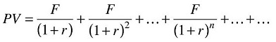
The present value (PV) of a security is the sum of its discounted cash flows, i.e.:

where Fn are the cash flows generated by the security, r is the applied discounting rate and n is the number of years for which the security is discounted.
All securities also have a market value, particularly on the secondary market. Market value is the price at which a security can be bought or sold.
Net present value (NPV) is the difference between present value and market value (V 0):
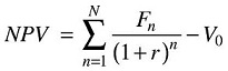
If the net present value of a security is greater than its market value, then it will be worth more in the future than the market has presently valued it at. Therefore, you will probably want to invest in it, i.e. to invest in the upside potential of its value.
If, however, the security’s present value is below its market value, then you should sell it at once, for its market value is sure to diminish.
2. ... to its fair value
If an imbalance occurs between a security’s market value and its present value, then efficient markets will seek to re-establish balance and reduce net present value to zero. Investors acting on efficient markets seek out investments offering positive net present value, in order to realise that value. When they do so, they push net present value towards zero, ultimately arriving at the fair value of the security.
3. Applying the concept of net present value to other investments
Up to this point, the discussion has been limited to financial securities. However, the concepts of present value and net present value can easily be applied to any investment, such as the construction of a new factory, the launch of a new product, the takeover of a competing company or any other asset that will generate positive and/or negative cash flows.
The concept of net present value can be interpreted in three different ways:
- the value created by an investment – for example, if the investment requires an outlay of €100 and the present value of its future cash flow is €110, then the investor has become €10 wealthier;
- the maximum additional amount that the investor is willing to pay to make the investment – if the investor pays up to €10 more, he has not necessarily made a bad deal, as he is paying up to €110 for an asset that is worth €110;
- the difference between the present value of the investment (€110) and its market value (€100).
Section 16.4 What does net present value depend on?
While net present value is obviously based on the amount and timing of cash flows, it is worth examining how it varies with the discounting rate.
The higher the discounting rate, the more future cash flow is depreciated and, therefore, the lower is the present value. Net present value declines in inverse proportion to the discounting rate, thus reflecting investor demand for a greater return (i.e. greater value attributed to time).
Take the following example of an asset (e.g. a financial security or a capital investment) with a market value of 2 and with cash flows as follows:
| Year | 1 | 2 | 3 | 4 | 5 |
| Cash flow | 0.8 | 0.8 | 0.8 | 0.8 | 0.8 |
A 20% discounting rate would produce the following discounting factors:
| Year | 1 | 2 | 3 | 4 | 5 |
| Discounting factor | 0.833 | 0.694 | 0.579 | 0.482 | 0.402 |
| Present value of cash flow | 0.67 | 0.56 | 0.46 | 0.39 | 0.32 |
As a result, the present value of this investment is about 2.40.1 As its market value is0.67 + 0.56 + 0.46 + 0.39 + 0.32 = 2.40. 2, its net present value is approximately 0.40.
If the discounting rate changes, the following values are obtained:
| Discounting rate | 0% | 10% | 20% | 25% | 30% | 35% |
| Present value of the investment | 4 | 3.03 | 2.39 | 2.15 | 1.95 | 1.78 |
| Market value | 2 | 2 | 2 | 2 | 2 | 2 |
| Net present value | 2 | 1.03 | 0.39 | 0.15 | −0.05 | −0.22 |
Which would then look like this graphically:

The higher the discounting rate (i.e. the higher the return demanded), the lower the net present value.
Section 16.5 Some examples of simplification of present value calculations
For those occasions when you are without your favourite spreadsheet program, you may find the following formulas handy in calculating present value.
1. The value of an annuity F over n years, beginning in year 1

or:

For the two formulas above, the sum of the geometric series can be expressed more simply as:

So, if F = 0.8, r = 20% and n = 5, then the present value is indeed 2.4.
Further,
 is equal to the sum of the first n discounting factors.
2. The value of a perpetuity
A perpetuity is a constant stream of cash flows without end. By adding this feature to the previous case, the formula then looks like this:
As n approaches infinity in the formula of the previous paragraph, this can be shortened to the following:

The present value of a €100 perpetuity discounted back at 10% per year is thus:
A €100 perpetuity discounted at 10% is worth €1000 in today’s euros. If the investor demands a 20% return, then the same perpetuity is worth €500.
3. The value of an annuity that grows at rate g for n years
In this case, the F 0 cash flow rises annually by g for n years.
Thus:

or:

Note: the first cash flow actually paid out is F 0 × (1 + g).
Thus, a security that has just paid out 0.8, and with this 0.8 growing by 10% each year for the four following years, has – at a discounting rate of 20% – a present value of:
4. The value of a perpetuity that grows at rate g (growing perpetuity)
As n approaches infinity, the previous formula can be expressed as follows:

As long as r > g. The present value is thus equal to the next year’s cash flow divided by the difference between the discounting rate and the annual growth rate.
For example, a security with an annual return of 0.8, growing by 10% annually to infinity, has, at a rate of 20%, PV = 0.8/(0.2 – 0.1) = 8.0.
Summary
Questions
Exercises
Answers