1. Building a business plan

The reader must realise that the business plan is the first stage in assessing the risks related to an investment. The purpose of the business plan is to model the firm’s most probable future, and it helps to identify the parameters that could significantly impact on a project’s value. For example, in certain industries where sales prices are not very important, the model will be based on gross margins, which are more stable than turnover.

Establishing a business plan helps to determine the project’s dependence upon factors over which investors have some influence, such as costs and/or sales price. It also outlines those factors that are beyond investors’ control, such as raw material prices, exchange rates, etc. Obviously, the more the business plan depends upon exogenous factors, the riskier it becomes.

2. Sensitivity analysis

One important risk analysis consists of determining how sensitive the investment is to different economic assumptions. This is done by holding all other assumptions fixed and then applying the present value to each different economic assumption. It is a technique that highlights the consequences of changes in prices, volumes, rising costs or additional investments on the value of projects.

Firms generally build three scenarios (pessimistic, realistic and optimistic). In certain sectors highly dependent on raw materials or other exogenous factors (such as the price of electricity), investment scenarios are deducted from predetermined macroeconomic scenarios.

The sensitivity analysis requires a good understanding of the sector of activity and its specific constraints. The industrial analysis must be rounded off with a more financial analysis of the investment’s sensitivity to the model’s technical parameters, such as the discount rate or terminal value (growth rate to infinity, see Chapter 31).

Practitioners usually build a sensitivity matrix, which offers an overview of the sensitivity of the investment’s NPV to the various assumptions.

Other companies prefer to focus on only one scenario, that is analysed in depth in order to keep managers of the project committed.

3. Assessment of the maximum risk

The investor, in particular if he is not familiar with the sector (which is usually the case for financial investors), may be tempted to build a very pessimistic scenario (worst-case scenario or crash test). Nevertheless, this scenario needs to remain realistic and thus cannot be a cumulative sensitivity analysis.

This exercise does not aim to determine a value but rather to assess the risk of failure (and potentially bankruptcy) of the project or to assess the additional investments that would then be needed. This scenario can also be useful to fix the maximum level of debt that the project can take.

1. Monte Carlo simulation

An even more elaborate variation of scenario analysis is the Monte Carlo simulation, which is based on more sophisticated mathematical tools and software. It consists of isolating a number of the project’s key variables or value drivers, such as turnover or margins, and allocating a probability distribution to each. The analyst enters all the assumptions about distributions of possible outcomes into a spreadsheet. The model then randomly samples from a table of predetermined probability distributions in order to identify the probability of each result.

Assigning probabilities to the investment’s key variables is done in two stages. First, influential factors are identified for each key variable. For example, with turnover, the analyst would also want to evaluate sales prices, market size, market share, etc. It is then important to look at available information (long-run trends, statistical analysis, etc.) to determine the uncertainty profile of each key variable using the values given by the influential factors.

Generally, there are several types of key variables, such as simple variables (e.g. fixed costs), compound variables (e.g. turnover = market × market share) or variables resulting from more complex, econometric relationships.

The investment’s net present value is shown as an uncertainty profile resulting from the probability distribution of the key variables, the random sampling of groups of variables and the calculation of net present value in this scenario.

Repeating the process many times gives us a clear representation of the NPV risk profile.

Once the uncertainty profile has been created, the question is whether to accept or reject the project. The results of the Monte Carlo method are not as clear cut as present value, and a lot depends upon the risk/reward trade-off that the investor is willing to accept. One important limitation of the method is the analysis of interdependence of the key variables; for example, how developments in costs are related to those in turnover.

2. The certainty equivalent

The certainty equivalent of a future cash flow is the certain amount that the investor would be ready to accept in exchange for an expected future risky cash flow. For example, if the investor is expecting a project to provide a 1000 cash flow in one year, given the risk he may consider trading this cash flow for the certainty of getting 600 in one year.

The certainty equivalent method leads to discounting using the risk-free rate and the certainty equivalent cash flows. The net present value of an investment can then be written as:

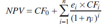
where e _i is the certainty equivalent factor of cash flow CF_i and r _F the risk-free rate.

To the best of our knowledge, this method remains rarely used in practice.

1. The limits of conventional analysis

Do not be confused by the variety of risk analysis techniques presented in the preceding section. In fact, all of these different techniques are based on the same principle. In the final analysis, simulations, the Monte Carlo or the certainty equivalent methods are just complex variations on the NPV criteria presented in Chapter 16.

Like NPV, conventional investment risk analyses are based on two fundamental assumptions:

• the choice of the anticipated future flow scenario; and
• the irreversible nature of the investment decision.

The second assumption brings up the limits of this type of analysis. Assuming that an investment is irreversible disregards the fact that corporate managers, once they get new information, generally have a number of options. They can abandon the investment halfway through if the project does not work out, they can postpone part of it or extend it if it has good development prospects, or they can use new technologies. The teams managing or implementing the projects constantly receive new information and can adapt to changing circumstances. In other words, the conventional approach to investment decisions ignores a key feature of many investment projects, namely flexibility.

It might be argued that the uncertainty of future flows has already been factored in via the mathematical hope criterion¹ and the discount rate, and therefore this should be enough to assess any opportunities to transform a project. However, it can be demonstrated that this is not necessarily so.

2. Real options

Industrial managers are not just passively exposed to risks. In many cases, they are able to react to ongoing events. They can increase, reduce or postpone their investment, and they exercise this right according to ongoing developments in prospective returns.

In fact, the industrial manager is in the same situation as the financial manager, who can increase or decrease his position in a security given predetermined conditions.

Industrial managers who have some leeway in managing an investment project are in the same position as financial managers holding an option.²

The flexibility of an investment thus has a value that is not reflected in conventional analysis. This value is simply that of the attached option. Obviously, this option does not take the form of the financial security with which you have already become familiar. It has no legal existence. Instead, it relates to industrial assets and is called a real option.

The potential flexibility of an investment, and therefore of the attached real options, is not always easy to identify. Industrial investors frequently do not realise or do not want to admit (especially when using a traditional investment criterion) that they do have some margin for manoeuvre. This is why it is often called a hidden option.

3. Real options categories

Given the potential value of hidden options, it is tempting to consider all investment uncertainties as a potential source of value. But the specific features of option contracts must not be overlooked. The following three factors are necessary to ensure that an investment project actually offers real options:

• The project must have a degree of uncertainty. The higher the underlying volatility, the greater the value of an option. If the standard deviation of the flows on a project is low, the value of the options will be negligible.
• Investors must be able to get more information during the course of the project, and this information must be sufficiently precise to be useful.
• Once the new information has been obtained, it must be possible to change the project significantly and irrevocably. If the industrial manager cannot use the additional information to modify the project, he does not really have an option but is simply taking a chance. In addition, the initial investment decision must also have a certain degree of irreversibility. If it can be changed at no cost, then the option has no value. And lastly, since the value of a real option stems from the investor’s ability to take action, any increase in investment flexibility generates value, since it can give rise to new options or increase the value of existing options.

Real options apply primarily to decisions to invest or divest, but they can appear at any stage of a company’s development. As a result, the review in this text of options theory is a broad outline, and the list of the various categories of real options is far from exhaustive.

The option to launch a new project corresponds to a call option on a new business. Its strike price is the start-up investment, a component that is very important in the valuation for many companies. In these cases, they are not valued on their own merits, but according to their ability to generate new investment opportunities, even though the nature and returns are still uncertain.

In acquiring stakes in Koolicar and Communauto in 2016, Peugeot has taken an option on the future development of the car-sharing business.

Similarly, R&D departments can be considered to be generators of real options embedded within the company. Any innovation represents the option to launch a new project or product. This is particularly true in the pharmaceutical industry. If the project is not profitable, this does not mean that the discovery has no value. It simply means that the discovery is out of the money. Yet this situation could change with further developments.

The option to develop or extend the business is comparable to the launch of a new project. However, during the initial investment phase decisions have to be made, such as whether to build a large factory to meet potentially strong demand or just a small plant to test the waters first.

A real options solution would be to build a small factory with an option to extend it if necessary. Flexibility is just as important in current operations as it is when deciding on the overall strategy of a project. Investments should be judged by their ability to offer recurring options throughout their lifecycle. Certain power stations, for example, can easily be adapted to run on coal or oil. This flexibility enhances their value, because they can easily be switched to a cheaper source of energy if prices fluctuate. Similarly, some auto plants need only a few adjustments in order to start producing different models.

The option to reduce or contract business is the opposite of the previous example. If the market proves smaller than expected, the investor can decide to cut back on production, thus reducing the corresponding variable costs. Indeed, he can also decide not to carry out part of the initial project, such as building a second plant. The implied sales price of the unrealised portion of the project consists of the savings on additional investments. This option can be described as a put option on a fraction of the project, even if the investment never actually materialises.

The option to postpone a project. The initial investment in the rights of an oil field is minimal in comparison with prospecting and extraction costs. It can thus be quite useful to defer the start of the project, for example until the business environment becomes more propitious (oil prices, operating costs, etc.). To a certain extent, this is similar to holding a well-known but not fully exploited brand.

Nonetheless, the option to defer the project’s start is valid only if the investor is able to secure ownership of the project from the outset. If not, his competitors may take on the project. In other words, the advantage of deferring the investment could be cancelled out by the risk of new market entrants.

Looking beyond the investment decision itself, option models can be used to determine the optimal date for starting up a project. In this case, the waiting period is similar to holding an American option on the project. The option’s value corresponds to the price of ensuring future ownership of the project (land, patents, licence, etc.).

The option to defer progress on the project is a continuation of the previous example. Some projects consist of a series of investments rather than just one initial investment. Should investors receive information casting doubt on a project that has already been launched, they may decide to put subsequent investments on hold, thus effectively halting further development. In fact, investors hold an option on the project’s further development at every call for more financing.

The option to abandon means that the industrial manager can decide to abandon the project at any time. Thus, hanging on to it today means keeping open the option to abandon at a later date. However, the reverse is not possible. This asymmetry is reflected in options theory, which assumes that a manager can sell his project at any time (but might not be able to buy it back once it is sold).

Such situations are analogous to the options theory of equity valuations that we will examine in Chapter 34. If the project is set up as a levered company, then the option to abandon corresponds to shareholders’ right to default. The value of this option is equal to that of equity, and it is exercised when the amount of outstanding debt is greater than the value of the project.

In the example below, the project includes an option to defer its launch (wait and see), an option to expand if it proves successful and an option to abandon it completely.

4. Evaluating real options

Option theory sheds light on the valuation of real options by stating that uncertainty combined with flexibility adds value to an industrial project. How appealing! It tells us that the higher the underlying volatility, and thus the risk, the greater the value of an option. This appears counterintuitive compared with the net present value approach, but remember that this value is very unstable. The time value of an option decreases as it reaches its exercise date, since the uncertainty declines with the accumulation of information on the environment.

Consider the case of a software publisher who is offered the opportunity to buy a licence to market connected homes software for £5m. If the publisher does not accept the deal right away, the licence will be offered to a rival. The software can be produced on the spot at a cost of £50m.

If the software is produced immediately, the company should be able to generate £2m in cash flows over the next year. The situation the following year, however, is far more uncertain, since one of the main equipment suppliers for connected homes is due to choose a new technological standard. If the standard chosen corresponds to that of the licence offered to our company, it can hope to generate a cash flow of £9m per year. If another standard is chosen, the cash flows will plunge to £1m per year. The management of our company estimates there is a 50% chance that the “right” standard will be chosen. As of the second year, the flows are expected to be constant to infinity.

The present value of the immediate launch of the product can easily be estimated with a discount rate of 10%. The anticipated flows are 0.5 × 9 + 0.5 × 1 = £5m from the second year on to infinity. Assuming that the first year’s flows are disbursed (or received) immediately, that second-year flows are disbursed (or received) at the very beginning of the second year and so on, the present value is 5/0.1 + 2 = £52m for a total cost of 50 + 5 = £55m. According to the NPV criterion, the project destroys £3m in value and the company should reject the licensing offer.

This would be a serious mistake!

If it buys the licence, the company can decide to produce the software whenever it wants to and can easily wait a year before investing in production. While this means giving up revenues of £2m in the first year, the company will have the advantage of knowing which standard the equipment supplier will have chosen. It can thus decide to produce only if the standard is suited to its product. If it is not, the company abandons the project and saves on development costs. The licence offered to the company thus includes a real option: the company is entitled to earn the flows on the project in exchange for investing in production.

The NPV approach assumes that the project will be launched immediately. That corresponds to the immediate exercise of the call option on the underlying instrument. This exercise destroys the time value. To assess the real value of the licence, we have to work out the value of the corresponding real option, i.e. the option of postponing development of the software.

The value of an option can be determined by the binomial method, which we described in greater detail in Chapter 23.

Imagine that the company has bought the licence and put off producing the software for a year. It now knows what standard the carrier has chosen. If the standard suits its purposes, it can immediately start up production at an NPV of 9 × (1 + 1/0.1) − 50 = £49m at that date. If the wrong standard is chosen, the NPV of developing the software falls to 
1 × (1 + 1/0.1) − 50 = −£39m, and the company drops the project (this investment is irreversible and has no hidden options). The value of the real option attached to the licence is thus £49m for a favourable outcome and 0 for an unfavourable outcome. Using a risk-free discount rate of 5%, the calculation for the initial value of the option is £23.3m, since:

Here is another look at the licensing offer. The licence costs £5m and the value of the real option is £23.3m, assuming development is postponed for one year. With this proviso, the company has been offered the equivalent of an immediate gain of 23.3 − 5 = £18.3m.

In this example, the difference between the two approaches is considerable. Legend has it that when an oil concession was once being auctioned off, one of the bidding companies offered a price that was less than a tenth of that of its competitor, quite simply because he had “forgotten” to factor in the real options!

This example assumed just one binomial alternative but, when attempting to quantify the value of real options in an investment, one is faced by a myriad of alternatives. More generally, the binomial model uses the replicating portfolio approach, which requires the use of quite sophisticated mathematical tools. Estimating volatility is always a problematic issue with respect to the concrete application of this methodology. In addition, the method requires defining a convenience yield that represents the interest in holding an asset at a certain point in time given its expected return.

In practice, the information derived from the quantification of real options is frequently not very significant when compared with a highly positive NPV in the initial scenario. However, when NPV is negative at the outset, one always has to consider the flexibility of the project by resorting to real options.

5. The expanded net present value

Since options allow us to analyse the various risks and opportunities arising from an investment, the project can be assessed as a whole. This is done by taking into account its two components – anticipated flows and real options. Some authors call this the expanded net present value (ENPV), which is the opposite of the “passive” NPV of a project with no options. ENPV is equal to the NPV grossed up with the value or real options of the investment.

When a project is very complex with several real options, the various options cannot be valued separately since they are often conditional and interdependent. If the option to abandon the project is exercised, then the option to reduce business obviously no longer exists and its value is nil. As a result, there is no additional value on options that are interdependent.

6. Conclusion

The predominant appeal of real options theory is its factoring of the value of flexibility that the traditional approaches ignore. The traditional net present value approach assumes that there is only one possible outcome. It does not take into account possible adaptive actions that could be taken by corporate managers. Real options fill this gap.

But do not get carried away; applying this method can be quite difficult because:

• not everyone knows how to use the mathematical models. This can create problems in communicating findings; and
• estimating some of the required parameters, such as volatility, opportunity costs, etc., can be complicated.

We trust that the reader will not mind being told that the use of these tools by practitioners is inversely correlated to the place devoted to them in this chapter: virtually systematic for scenarios, less often for the Monte Carlo method and very rarely for real options.

Summary

Questions

Exercise

Answers

Notes

Bibliography