
Scales are functions provided by D3.js that map a set of values to another set of values. The input set of values is referred to as the domain, and the output is the range. The basic reason for the existence of scales is to prevent us from coding loops, and doing a lot of math to make these conversions happen. This is a very useful thing.
There are three general categories of scales: quantitative, ordinal, and time-scale. Within each category of scale, D3.js provides a number of concrete implementations that exist for accomplishing a specific type of mapping data useful for data visualization.
Covering examples of every type of scale would consume more space than is available in this book, and at the same time become tedious to read. We will examine several common scales that are used—kind of the 80/20 rule, where the few we cover here will be used most of the time you use scales.
Linear scales are a type of quantitative scale that are arguably the most commonly used ones. The mapping performed is linear in that the output range is calculated using a linear function of the input domain.
A good example of using a linear scale is the scenario with our The Walking Dead viewership data. We need to draw bars from this data; but if we use the code that we used earlier in the book, our bars will be extremely tall since that code has a one to one mapping between the value and the pixels.
Let's assume that our area for the bars on the graph has a height of 400 pixels. We would like to map the lowest viewership value to a bar that is 100 pixels tall, and map the largest viewership value to 400. The following example performs this task:
Note
bl.ock (5.5): http://goo.gl/dgg0zf
The code starts, as with the CSV example, by loading that data and mapping/converting it. The next task is to determine the minimum and maximum viewership values:
var viewership = mappedAndConverted.map(function (d) {
     return d.USViewers;
});
var minViewership = d3.min(viewership);
var maxViewership = d3.max(viewership);
Next, we define several variables representing the minimum and maximum height that we would like for the bars:
var minBarHeight = 100, maxBarHeight = 400;
The scale is then created as follows:
var yScale = d3.scale
    .linear()
    .domain([minViewership, maxViewership])
    .range([minBarHeight, maxBarHeight]);
We can now use the yScale object as though it is a function. The following will log the results of scaling the minimum and maximum viewership values:
console.log(minViewership + " -> " + yScale(minViewership));
console.log(maxViewership + " -> " + yScale(maxViewership));
Examining the console output, we can see that the scaling resulted in the expected values:
"12270000 -> 100"
"17290000 -> 400"
Ordinal scales are, in a way, similar to dictionary objects. The values in the domain and range are discrete. There must be an entry in the range for every unique input value, and that value must have a mapping to a single value in the range.
There are several common uses for ordinal scales, and we will examine four common uses that we will use throughout the remainder of this book.
Open the following link for an example of an ordinal scale. This example does not use the data from The Walking Dead, and simply demonstrates the mapping of string literals representing primary colors into the corresponding color codes.
Note
bl.ock (5.6): http://goo.gl/DezcUN
The scale is created as follows:
var colorScale = d3.scale.ordinal()
    .domain(['red', 'green', 'blue'])
    .range(['#ff0000', '#00ff00', '#0000ff']);
We can now pass any of the range values to the colorScale, as demonstrated with the following:
console.log(colorScale('red'),
    colorsScale('green'),
    colorScale('blue'));
Examining the console output, we can see the results of this mapping as follows:
"#ff0000"
"#00ff00"
"#0000ff"
D3.js comes with several special built-in scales that are referred to as categorical scales. It sounds like a fancy term, but they are simply mappings of a set of integers to unique colors (unique within that scale).
These are useful when you have a set of sequential 0-based integer keys in your data, and you want to use a unique color for each, but you do not want to manually create all the mappings (like we did for the three strings in the previous example).
Open the following link for an example of using a 10 color categorical scale:
Note
bl.ock (5.7): http://goo.gl/RSW9Qa
The preceding example renders 10 adjacent rectangles, each with a unique color from a category10() color scale. You will see this in your browser when executing this example.
The example starts by creating an array of 10 integers from 0 to 9.
var data = d3.range(0, 9);
var colorScale = d3.scale.category10();
Now we can bind the integers to the rectangles, and set the fill for each by passing the value to the colorScale function:
var svg = d3.select('body')
    .append('svg')
    .attr({width: 200, height: 20});

svg.selectAll('rect')
    .data(data)
    .enter()
    .append('rect')
    .attr({
        fill: function(d) { return colorScale(d); },
        x: function(d, i) { return i * 20 },
        width: 20,
        height: 20
    });
D3.js provides four sets of categorical color scales that can be used depending upon your scenario. You can take a look at them on the D3.js documentation page at https://github.com/mbostock/d3/wiki/Ordinal-Scales.
In Chapter 4, Creating a Bar Graph, when we drew the graph we calculated the positions of the bars based upon a fixed bar size and padding. This is actually a very inflexible means of accomplishing this task. D3.js gives us a special scale that we can use, given the domain values and essentially a width, that will tell us the start and end values for each bar such that all the bars fit perfectly within the range!
Let's take a look using this special scale with the following example:
Note
bl.ock (5.8): http://goo.gl/OG3g7S
This example creates a simple ordinal scale specifying the range using the .rangeBands() function instead of .range(). The entire code of the example is as follows:
var bands = d3.scale.ordinal()
    .domain([0, 1, 2])
    .rangeBands([0, 100]);
console.log(bands.range());
console.log(bands.rangeBand());
The .range() function will return an array with values representing the extents of an equal number of evenly-spaced divisions of the range specified to .rangeBands(). In this case, the width of the range is 100, and there are three items specified in the domain; hence, the result is the following:
[0, 33.333333333333336, 66.66666666666667]
Technically, this result is the values that represent the start of each band. The width of each band can be found using the .rangeBand() function, in this case returning the following:
33.333333333333336
This width may seem simplistic. Why have this function if we can just calculate the difference between two adjacent values in the result of .range()? To demonstrate, let's look at a slight modification of this example, available at the following link.
Note
bl.ock (5.9): http://goo.gl/JPsuqh
This makes one modification to the call to .rangeBands(), adding an additional parameter that specifies the padding that should exist between the bars:
var bands = d3.scale.ordinal()
    .domain([0, 1, 2])
    .rangeRoundBands([0, 100], 0.1);
The output differs slightly due to the addition of padding between the bands:
[3.2258064516129035, 35.483870967741936, 67.74193548387096]
29.032258064516128
The width of each band is now 29.03, with a padding of 3.23 between bands (including on the outside of the two outer bands).
The value for padding is a value between 0.0 (the default, and which results in a padding of 0) and 1.0, resulting in bands of width 0.0. A value of 0.5 makes the padding the same width as each band.
Now we pull everything from the chapter together to render a bar graph of the viewership across all the episodes of The Walking Dead:
Note
bl.ock (5.10): http://goo.gl/T8d6OU
The output of the preceding example is as follows:
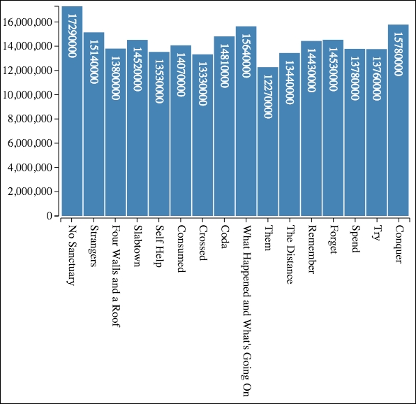
Now let's step through how this is created. After loading the data from the JSON file, the first thing that is performed is the extraction of the USViewership values and the determining of the maximum value:
var viewership = data.map(function (d) {
    return d.USViewers;
});

var maxViewers = d3.max(viewership);
Then various variables, which represent various metrics for the graph, and the main SVG element are created:
var margin = { top: 10, right: 10, bottom: 260, left: 85 };

var graphWidth = 500, graphHeight = 300;

var totalWidth = graphWidth + margin.left + margin.right;
var totalHeight = graphHeight + margin.top + margin.bottom;

var axisPadding = 3;

var svg = d3.select('body')
    .append('svg')
    .attr({ width: totalWidth, height: totalHeight });
The container for holding the bars is created next:
var mainGroup = svg
    .append('g')
    .attr('transform', 'translate(' + margin.left + ',' +
                                      margin.top + ")");
Now we create an ordinal scale for the bars using .rangeBands(). We will use this to calculate the bar position and padding:
var bands = d3.scale.ordinal()
    .domain(viewership)
    .rangeBands([0, graphWidth], 0.05);
We also require a scale to calculate the height of each bar:
var yScale = d3.scale
    .linear()
    .domain([0, maxViewers])
    .range([0, graphHeight]);
The following function is used by the selection that creates the bars to position each of them:
function translator(d, i) {
    return "translate(" + bands.range()[i] + "," +
                          (graphHeight - yScale(d)) + ")";
}
Now we create the groups for the content of each bar:
var barGroup = mainGroup.selectAll('g')
    .data(viewership)
    .enter()
    .append('g')
    .attr('transform', translator);
Next we append the rectangle for the bar:
barGroup.append('rect')
    .attr({
        fill: 'steelblue',
        width: bands.rangeBand(),
        height: function(d) { return yScale(d); }
    });
And then add a label to the bar to show the exact viewership value:
barGroup.append('text')
    .text(function(d) { return d; })
    .style('text-anchor', 'start')
    .attr({
        dx: 10,
        dy: -10,
        transform: 'rotate(90)',
        fill: 'white'
    });
The bars are now complete, so we move on to creating both the axes. We start with the left axis:
var leftAxisGroup = svg.append('g');
leftAxisGroup.attr({
    transform: 'translate(' + (margin.left - axisPadding) + ',' +
                               margin.top + ')'
});

var yAxisScale = d3.scale
    .linear()
    .domain([maxViewers, 0])
    .range([0, graphHeight]);

var leftAxis = d3.svg.axis()
    .orient('left')
    .scale(yAxisScale);
var leftAxisNodes = leftAxisGroup.call(leftAxis);
styleAxisNodes(leftAxisNodes);
And now create a bottom axis which displays the titles:
var titles = data.map(function(d) { return d.Title; });
var bottomAxisScale = d3.scale.ordinal()
    .domain(titles)
    .rangeBands([axisPadding, graphWidth + axisPadding]);

var bottomAxis = d3.svg
    .axis()
    .scale(bottomAxisScale)
    .orient("bottom");

var bottomAxisX = margin.left - axisPadding;
var bottomAxisY = totalHeight - margin.bottom + axisPadding;

var bottomAxisGroup = svg.append("g")
    .attr({ transform: 'translate(' + bottomAxisX + ',' + bottomAxisY + ')' });

var bottomAxisNodes = bottomAxisGroup.call(bottomAxis);
styleAxisNodes(bottomAxisNodes);

bottomAxisNodes.selectAll("text")
    .style('text-anchor', 'start')
    .attr({
        dx: 10,
        dy: -5,
        transform: 'rotate(90)'
});
The following function is reusable code for styling the axes:
function styleAxisNodes(axisNodes) {
    axisNodes.selectAll('.domain')
        .attr({
            fill: 'none',
            'stroke-width': 1,
            stroke: 'black'
        });
    axisNodes.selectAll('.tick line')
        .attr({
            fill: 'none',
            'stroke-width': 1,
            stroke: 'black'
        });
}