Our first example will demonstrate how to construct a force-directed graph. The online example is available at the following link:

All our force-directed graphs will start by loading data that represents a network. This example uses the data at https://gist.githubusercontent.com/d3byex/5a8267f90a0d215fcb3e/raw/ba3b2e3065ca8eafb375f01155dc99c569fae66b/uni_network.json.

The following are the contents of the file at the preceding link:

{
  "nodes": [
    { "name": "Mike" },
    { "name": "Marcia" },
    { "name": "Chrissy" },
    { "name": "Selena" },
    { "name": "William" },
    { "name": "Mikael" },
    { "name": "Bleu" },
    { "name": "Tagg" },
    { "name": "Bob" },
    { "name": "Mona" }
  ],
  "edges": [
    { "source": 0, "target":  1 },
    { "source": 0, "target":  4 },
    { "source": 0, "target":  5 },
    { "source": 0, "target":  6 },
    { "source": 0, "target":  7 },
    { "source": 1, "target":  2 },
    { "source": 1, "target":  3 },
    { "source": 1, "target":  5 },
    { "source": 1, "target":  8 },
    { "source": 1, "target":  9 },
  ]
}

The force-directed layout algorithms in D3.js require the data to be in this format. This needs to be an object with a nodes and an edges property. The nodes property can be an array of any other objects you like to use. These are typically your data items.

The edges array must consist of objects with both source and target properties, and the value for each is the index into the nodes array of the source and target nodes. You can add other properties, but we need to supply at least these two.

To start rendering the graph, we load this data and get the main SVG element created:

var url = 'https://gist.githubusercontent.com/d3byex/5a8267f90a0d215fcb3e/raw/ba3b2e3065ca8eafb375f01155dc99c569fae66b/uni_network.json';
d3.json(url, function(error, data) {
    var width = 960, height = 500;
    var svg = d3.select('body').append('svg')
        .attr({
            width: width,
            height: height
        });

The next step is to create the layout for the graph using d3.layout.force(). There are many options, several of which we will explore over the course of our examples, but we start with the following:

var force = d3.layout.force()
    .nodes(data.nodes)
    .links(data.edges)
    .size([width, height])
    .start();

This informs the layout about the location of the nodes and links using the .node() and .link() functions respectively. The call to .size() informs the layout about the area to constrain the layout within and has two effects on the graph: the gravitational center and the initial random position.

The call to .start() begins the simulation, and must be called after the layout is created and the nodes and links are assigned. If the nodes and links change later, it can be called again to restart the simulation. Note that the simulation starts after this function returns, not immediately. So, you can still make other changes to the visual.

Now we can render the links and nodes:

var edges = svg.selectAll('line')
    .data(data.edges)
    .enter()
    .append('line')
    .style('stroke', '#ccc')
    .style('stroke-width', 1);

var colors = d3.scale.category20();
var nodes = svg
    .selectAll('circle')
    .data(data.nodes)
    .enter()
    .append('circle')
    .attr('r', 10)
    .attr('fill', function(d, i) {
        return colors(i);
    })
    .call(force.drag);

Note that we also chained the .call() function passing it a reference to the force.drag function of our layout. This function is provided by the layout object to easily allow us a means of dragging the nodes in the network.

There is one more step required. A force layout is a simulation and consists of a sequence of ticks that we must handle. Each tick represents that the layout algorithm has passed over the nodes and recalculated their positions, and this gives us the opportunity to reposition the visuals.

To hook into the ticks, we can use the force.on() function, telling it that we want to listen to tick events, and on each event, call a function to allow us to reposition our visuals. The following is our function for this activity:

force.on('tick', function() {
    edges.attr({
        x1: function(d) { return d.source.x; },
        y1: function(d) { return d.source.y; },
        x2: function(d) { return d.target.x; },
        y2: function(d) { return d.target.y; }
    });

    nodes.attr('cx', function(d) { return d.x; })
         .attr('cy', function(d) { return d.y; });
});

On each tick, we need to reposition each node and edge appropriately. Notice how we are doing this. D3.js has added to our data x and a y properties, which are the calculated position. It also has added a px and py property to each data node, which represents the previous x and y position.

On running this, the output will be similar to the following:

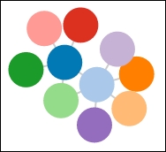
Every time this example is executed, the nodes will finish in a different position. This is due to the algorithm specifying a random start position for each node.

The nodes are very close in this example, to the point where the links are almost not visible. But it is possible to drag the nodes with the mouse, which will expose the links. Also notice that the layout is executed while you drag and the nodes snap back to the middle when the dragged node is released.