
In this chapter, we will examine a specific type of layout known as a force-directed graph. These are a type of visualization that are generally utilized to display network information: interconnected nodes.
A particularly common type of network visualization is of the relationships within a social network. A visualization of a social network can help you understand how different people have formed various relationships. These include links between others as well as the way groups of people form clusters or cliques of friends and how those groups interrelate.
D3.js provides extensive capabilities for creating very complex network visualizations using force-directed networks. We will overview a number of representative examples of these graphs, cover a little bit of the theory of how they operate, and dive into a few examples to demonstrate their creation and usage.
Specifically, in this chapter we will cover the following topics:
- A brief overview of force-directed graphs
- Creating a basic force-directed graph
- Modifying the length of the links
- Forcing nodes to move away from each other
- Labeling the nodes
- Forcing nodes to stay in place
- Expressing directionality and type with link visuals
There are a number of means of rendering network data. A particularly common one, which we will examine in this chapter, is to use a class of algorithms known as force-directed layouts.
These algorithms position the nodes in the graph in a two or three dimensional space. The positioning is performed by assigning forces along edges and nodes, and then these forces are used to simulate moving the nodes into a position where the amount of energy in the entire system is minimized.
The following is a representative picture of a force-directed graph from a Wiki. Nodes are pages, and the lines between the nodes represent the links between the pages. Node size varies based on the number of links in/out of a particular node:
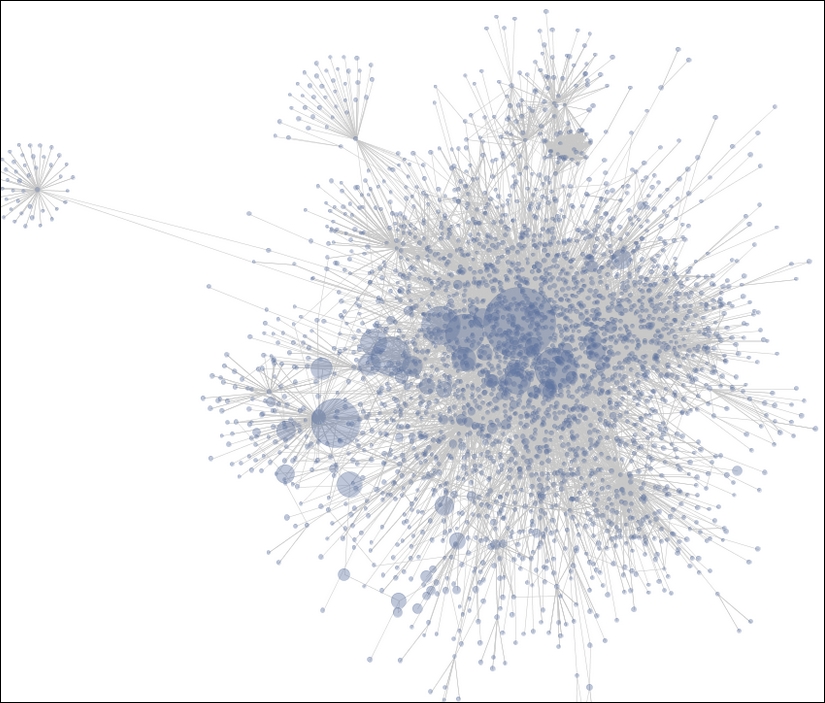
The fundamental components of a force-directed graph are the nodes in the graph and the relations between those nodes. The graph is iteratively laid out, usually animated during the process, and can take quite a few iterations to stabilize.
The force layout algorithm in D3.js takes into account a number of factors. A few of the important parameters of the algorithm and how they influence the simulation are the following:
- Size (width and height): This represents an overall size of the diagram, and a center of gravity, normally the center of the diagram. Nodes in the diagram will tend to move towards this point. If nodes do not have an initial
xandyposition, then they will be placed randomly in a position between 0 and width in thexdirection and height in theydirection. - Charge: This describes how much a node attracts other nodes. Negative values push away other nodes, and positive numbers attract. The larger the value in either direction, the stronger is the force in that direction.
- Charge distance: This specifies the maximum distance over which charge has effect (it defaults to infinity). Smaller values assist in performance of the layout, and result in a more localized layout of nodes in clusters.
- Friction: Represents an amount of velocity delay. This value should be in the range of
[0, 1]. At each tick of the layout, the velocity of every node is multiplied by this value. Using a value of 0 therefore, freezes all nodes in place, and1is a frictionless environment. Values in between eventually slow the nodes to a point where overall motion is small enough, and the simulation can be considered complete as the total amount of movement falls below the layout threshold at which point the graph is referred to as stable. - Link distance: This specifies a desired distance between nodes at the end of the simulation. At each tick of the simulation, the distance between linked nodes is compared to this value, and nodes move towards or away from each other to try to reach the desired distance.
- Link strength: This is a value in the range of
[0, 1], specifying how stretchable the link distance is during the simulation. A value of 0 is rigid and1is completely flexible. - Gravity: This specifies an attraction of each node to the center of the layout. This is a weak geometric constraint. That is, the higher the overall gravity, the further away it is from the center of the rendering. This value is useful for keeping layouts relatively centered in the diagram and in keeping disconnected nodes from flying out to infinity.
We will go over enough of these parameters to get a good feel for making useful visualizations.
Note
More detail on all the layout parameters is available at https://github.com/mbostock/d3/wiki/Force-Layout.
In addition to the parameters that facilitate the actual layout of the nodes, it is also possible to use other visual in a force-directed graph to convey various values in the underlying information:
- The color of a node can be used to distinguish nodes of particular types, such as people versus employers, or by their relation, such as all persons who work at a particular employer, or how many degrees of separation the node is from another node.
- The size of a node, which generally represents the magnitude of importance of the node. Often the number of links influence the size of a node.
- The thickness of the rendering of a link can be used to demonstrate that certain links have more influence than others or that the links are of particular types, that is, highways versus railways.
- The directionality of link, showing that the link has either no directionality or is one or bi-directional.