The concepts of short-time Fourier analysis and synthesis have been widely described in the literature [Por76, Cro80, CR83]. We will briefly summarize the basics and define our notation of terms for application to digital audio effects.
The short-time Fourier transform (STFT) of the signal x(n) is given by
7.2 ![]()
7.3 ![]()
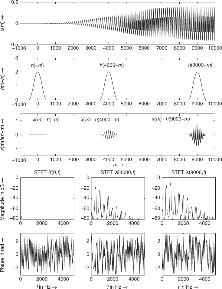
X(n, k) is a complex number and represents the magnitude |X(n, k)| and phase φ(n, k) of a time-varying spectrum with frequency bin (index) 0 ≤ k ≤ N − 1 and time index n. Note that the summation index is m in (7.1). At each time index n the signal x(m) is weighted by a finite length window h(n − m). Thus the computation of (7.1) can be performed by a finite sum over m with an FFT of length N. Figure 7.3 shows the input signal x(m) and the sliding window h(n − m) for three time indices of n. The middle plot shows the finite length windowed segments x(m) · h(n − m). These segments are transformed by the FFT, yielding the short-time spectra X(n, k) given by (7.1). The lower two rows in Figure 7.3 show the magnitude and phase spectra of the corresponding time segments.
Figure 7.3 Sliding analysis window and short-time Fourier transform.
7.2.1 Filter Bank Summation Model
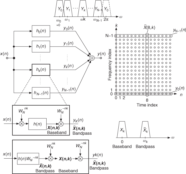
The computation of the time-varying spectrum of an input signal can also be interpreted as a parallel bank of N bandpass filters, as shown in Figure 7.4, with impulse responses and Fourier transforms given by
7.5 ![]()
Each bandpass signal yk(n) is obtained by filtering the input signal x(n) with the corresponding bandpass filter hk(n). Since the bandpass filters are complex-valued, we get complex-valued output signals yk(n), which will be denoted by
These filtering operations are performed by the convolutions
From (7.6) and (7.8) it is important to notice that
7.9 ![]()
Based on Equations (7.7) and (7.8) two different implementations are possible, as shown in Figure 7.4. The first implementation is the so-called complex baseband implementation according to (7.8). The baseband signals X(n, k) (short-time Fourier transform) are computed by modulation of x(n) with ![]() and lowpass filtering for each channel k. The modulation of X(n, k) by
and lowpass filtering for each channel k. The modulation of X(n, k) by ![]() yields the bandpass signal
yields the bandpass signal ![]() . The second implementation is the so-called complex bandpass implementation, which filters the input signal with hk(n) given by (7.4), as shown in the lower left part of Figure 7.4. This implementation leads directly to the complex-valued bandpass signals
. The second implementation is the so-called complex bandpass implementation, which filters the input signal with hk(n) given by (7.4), as shown in the lower left part of Figure 7.4. This implementation leads directly to the complex-valued bandpass signals ![]() . If the equivalent baseband signals X(n, k) are necessary, they can be computed by multiplication with
. If the equivalent baseband signals X(n, k) are necessary, they can be computed by multiplication with ![]() . The operations for the modulation by
. The operations for the modulation by ![]() yielding X(n, k) and back modulation by
yielding X(n, k) and back modulation by ![]() (lower left part of Figure 7.4) are only shown to point out the equivalence of both implementations.
(lower left part of Figure 7.4) are only shown to point out the equivalence of both implementations.
Figure 7.4 Filter bank description of the short-time Fourier transform. Two implementations of the kth channel are shown in the lower left part. The discrete-time and discrete-frequency plane is shown in the right part. The marked bandpass signals yk(n) are the horizontal samples ![]() . The different frequency bands Yk corresponding to each bandpass signal are shown on top of the filter bank. The frequency bands for the baseband signal X(n, k) and the bandpass signal
. The different frequency bands Yk corresponding to each bandpass signal are shown on top of the filter bank. The frequency bands for the baseband signal X(n, k) and the bandpass signal ![]() are shown in the lower right part.
are shown in the lower right part.
The output sequence y(n) is the sum of the bandpass signals according to
7.11 
The output signals yk(n) are complex-valued sequences ![]() . For a real-valued input signal x(n) the bandpass signals satisfy the property
. For a real-valued input signal x(n) the bandpass signals satisfy the property ![]() . For a channel stacking with
. For a channel stacking with ![]() we get the frequency bands shown in the upper part of Figure 7.4. The property
we get the frequency bands shown in the upper part of Figure 7.4. The property ![]() , together with the channel stacking can be used for the formulation of real-valued bandpass signals (real-valued kth channel)
, together with the channel stacking can be used for the formulation of real-valued bandpass signals (real-valued kth channel)
7.12 ![]()
7.13 ![]()
7.14 ![]()
This leads to
7.15 ![]()
7.16 
7.17 
Besides a dc and a highpass channel we have N/2 − 1 cosine signals with fixed frequencies ωk and time-varying amplitude and phase. This means that we can add real-valued output signals ![]() k(n) to yield the output signal
k(n) to yield the output signal

This interpretation offers analysis of a signal by a filter bank, modification of the short-time spectrum ![]() on a sample-by-sample basis and synthesis by a summation of the bandpass signals yk(n). Due to the fact that the baseband signals are bandlimited by the lowpass filter h(n), a sampling rate reduction can be performed in each channel to yield X(sR, k), where only every Rth sample is taken and s denotes the new time index. This leads to a short-time transform X(sR, k) with a hop size of R samples. Before the synthesis upsampling and interpolation filtering have to be performed [CR83].
on a sample-by-sample basis and synthesis by a summation of the bandpass signals yk(n). Due to the fact that the baseband signals are bandlimited by the lowpass filter h(n), a sampling rate reduction can be performed in each channel to yield X(sR, k), where only every Rth sample is taken and s denotes the new time index. This leads to a short-time transform X(sR, k) with a hop size of R samples. Before the synthesis upsampling and interpolation filtering have to be performed [CR83].
7.2.2 Block-by-block Analysis/synthesis Model
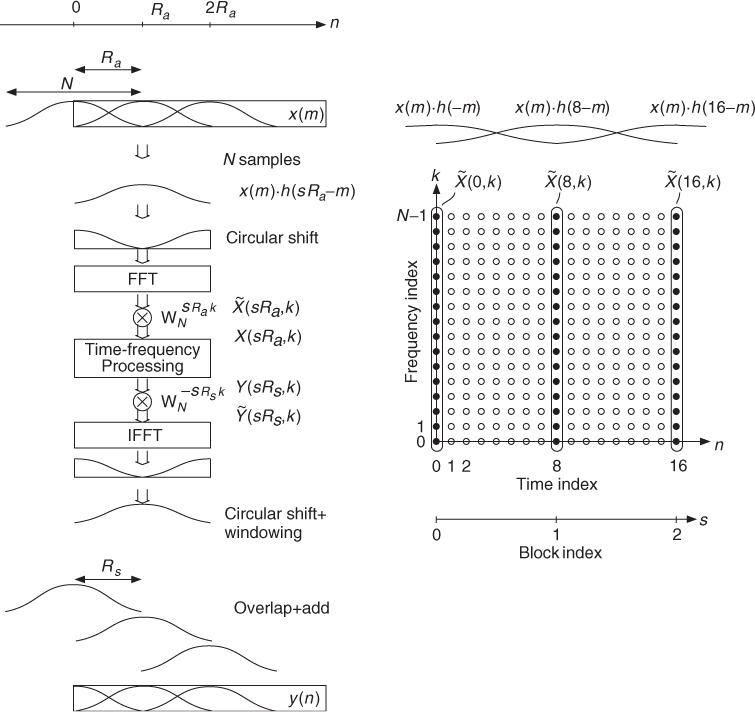
A detailed description of a phase vocoder implementation using the FFT can be found in [Por76, Cro80, CR83]. The analysis and synthesis implementations are precisely described in [(CR83, p. 318, Figure 7.19 and 7.19 p. 321, Figure 7.20)]. A simplified analysis and synthesis implementation, where the window length is less or equal to the FFT length, were proposed in [Cro80]. The analysis and synthesis algorithm and the discrete-time and discrete-frequency plane are shown in Figure 7.5. The analysis algorithm [Cro80] is given by
7.19 
7.20 
7.21 ![]()
7.22 ![]()
where the short-time Fourier transform is sampled every Ra samples in time and s denotes the time index of the short-time transform at the decimated sampling rate. This means that the time index is now n = sRa, where Ra denotes the analysis hop size. The analysis window is denoted by h(n). Notice that X(n, k) and ![]() in the FFT implementation can also be found in the filter bank approach. The circular shift of the windowed segment before the FFT and after the IFFT is derived in [CR83] and provides a zero-phase analysis and synthesis regarding the center of the window. Further details will be discussed in the next section. Spectral modifications in the time-frequency plane can now be done, which yields Y(sRs, k), where Rs is the synthesis hop size. The synthesis algorithm [Cro80] is given by
in the FFT implementation can also be found in the filter bank approach. The circular shift of the windowed segment before the FFT and after the IFFT is derived in [CR83] and provides a zero-phase analysis and synthesis regarding the center of the window. Further details will be discussed in the next section. Spectral modifications in the time-frequency plane can now be done, which yields Y(sRs, k), where Rs is the synthesis hop size. The synthesis algorithm [Cro80] is given by
where f(n) denotes the synthesis window. Finite length signals ys(n) are derived from inverse transforms of short-time spectra Y(sRs, k). These short-time segments are weighted by the synthesis window f(n) and then added by the overlap-add procedure given by (7.23) (see Figure 7.5).
Figure 7.5 Phase vocoder using the FFT/IFFT for the short-time Fourier transform. The analysis hop size Ra determines the sampling of the two-dimensional time-frequency grid. Time-frequency processing allows the reconstruction with a synthesis hop size Rs.