
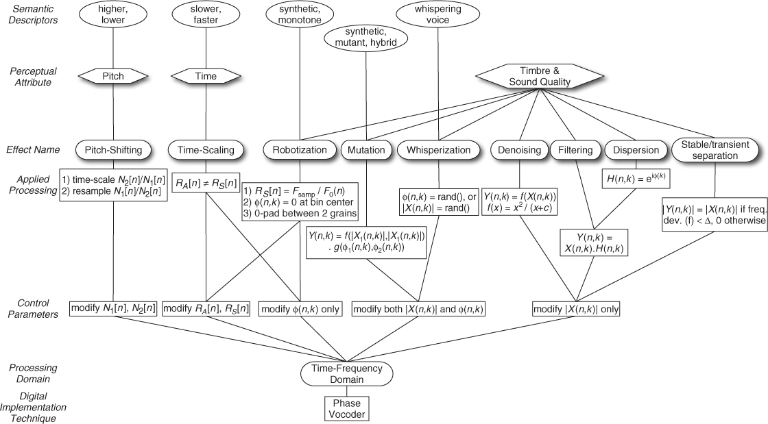
The following subsections will describe several modifications of a time-frequency representation before resynthesis in order to achieve audio effects. Most of them use the FFT analysis followed by either a summation of sinusoids or an IFFT synthesis, which is faster or more adapted to the effect. But all implementations give equivalent results and can be used for audio effects. Figure 7.19 provides a summary of those effects, with their relative operation(s) and the perceptual attribute(s) that are mainly modified.
Figure 7.19 Summary of time-frequency domain digital audio effects, with their relative operations and the perceptual attributes that are mainly modified.
7.4.1 Time-frequency Filtering
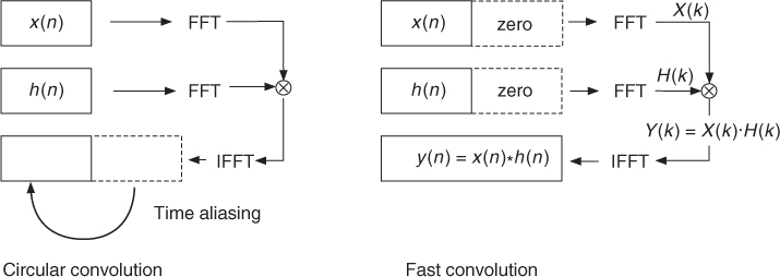
Filtering a sound can be done with recursive (IIR) or non-recursive (FIR) filters. However, a musician would like to define or even to draw a frequency response which represents the gain for each frequency band. An intuitive way is to use a time-frequency representation and attenuate certain zones, by multiplying the FFT result in every frame by a filtering function in the frequency domain. One must be aware that in that case we are making a circular convolution (during the FFT–inverse FFT process), which leads to time aliasing, as shown in Figure 7.20. The alternative and exact technique for using time-frequency representations is the design of an FIR impulse response from the filtering function. The convolution of the signal segment x(n) of length N with the impulse response of the FIR filter of length N + 1 leads to 2N-point sequence y(n) = x(n) * h(n). This time-domain convolution or filtering can be performed more efficiently in the frequency domain by multiplication of the corresponding FFTs Y(k) = X(k) · H(k). This technique is called fast convolution (see Figure 7.20) and is performed by the following steps:
1. Zero-pad the signal segment x(n) and the impulse response h(n) up to length 2N.
2. Take the 2N-point FFT of these two signals.
3. Perform multiplication Y(k) = X(k) · H(k) with k = 0, 1, …, 2N − 1.
4. Take the 2N-point IFFT of Y(k), which yields y(n) with n = 0, 1, …, 2N − 1.
Figure 7.20 Circular convolution and fast convolution.
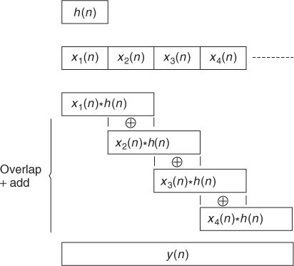
Now we can work with successive segments of length N of the original signal (which is equivalent to using a rectangular window), zero-pad each segment up to the length 2N and perform the fast convolution with the filter impulse response. The results of each convolution are added in an overlap-add procedure, as shown in Figure 7.21. The algorithm can be summarized as:
1. Start from an FIR filter of length N + 1, zero pad it to 2N and take its FFT ⇒ H(k).
2. Partition the signal into segments xi(n) of length N and zero-pad each segment up to length 2N.
3. For each zero-padded segment si(n) perform the FFT Xi(k) with k = 0, 1, …, 2N − 1.
4. Perform the multiplication Yi(k) = Xi(k) · H(k).
5. Take the inverse FFT of these products Yi(k).
6. Overlap-add the convolution results (see Figure 7.21).
The following M-file 7.7 demonstrates the FFT filtering algorithm.
M-file 7.7 (VX_filter.m)
% VX_filter.m [DAFXbook, 2nd ed., chapter 7]
%===== This program performs time-frequency filtering
%===== after calculation of the fir (here band pass)
clear; clf
%----- user data -----
fig_plot = 0; % use any value except 0 or [] to plot figures
s_FIR = 1280; % length of the fir [samples]
s_win = 2*s_FIR; % window size [samples] for zero padding
[DAFx_in, FS] = wavread(‘la.wav’);
%----- initialize windows, arrays, etc -----
L = length(DAFx_in);
DAFx_in = [DAFx_in; zeros(s_win-mod(L,s_FIR),1)] ...
/ max(abs(DAFx_in)); % 0-pad & normalize
DAFx_out = zeros(length(DAFx_in)+s_FIR,1);
grain = zeros(s_win,1); % input grain
vec_pad = zeros(s_FIR,1); % padding array
%----- initialize calculation of fir -----
x = (1:s_FIR);
fr = 1000/FS;
alpha = -0.002;
fir = (exp(alpha*x).*sin(2*pi*fr*x))'; % FIR coefficients
fir2 = [fir; zeros(s_win-s_FIR,1)];
fcorr = fft(fir2);
%----- displays the filter' simpulse response -----
if(fig_plot)
figure(1); clf;
subplot(2,1,1); plot(fir); xlabel(‘n [samples] ightarrow’);
ylabel(‘h(n) ightarrow’); axis tight;
title(‘Impulse response of the FIR’)
subplot(2,1,2);
plot((0:s_FIR-1)/s_FIR*FS, 20*log10(abs(fft(fftshift(fir)))));
xlabel(‘k ightarrow’); ylabel(‘|F(n,k)| / dB ightarrow’);
title(‘Magnitude spectrum of the FIR’); axis([0 s_FIR/2, -40, 50])
pause
end
tic
%UUUUUUUUUUUUUUUUUUUUUUUUUUUUUUUUUUUUUUU
pin = 0;
pout = 0;
pend = length(DAFx_in) - s_FIR;
while pin<pend
grain = [DAFx_in(pin+1:pin+s_FIR); vec_pad];
%===========================================
ft = fft(grain) .* fcorr;
grain = (real(ifft(ft)));
%===========================================
DAFx_out(pin+1:pin+s_win) = ...
DAFx_out(pin+1:pin+s_win) + grain;
pin = pin + s_FIR;
end
%UUUUUUUUUUUUUUUUUUUUUUUUUUUUUUUUUUUUUUU
toc
%----- listening and saving the output -----
% DAFx_in = DAFx_in(s_win+1:s_win+L);
DAFx_out = DAFx_out / max(abs(DAFx_out));
soundsc(DAFx_out, FS);
wavwrite(DAFx_out, FS, ‘la_filter.wav’);
Figure 7.21 FFT filtering.
The design of an N-point FIR filter derived from frequency-domain specifications is a classical problem of signal processing. A simple design algorithm is the frequency sampling method [Zöl05].
7.4.2 Dispersion
When a sound is transmitted over telecommunications lines, some of the frequency bands are delayed. This spreads a sound in time, with some components of the signal being delayed. It is usually considered a default in telecommunications, but can be used musically. This dispersion effect is especially significant on transients, where the sound loses its coherence, but can also blur the steady-state parts. Actually, this is what happens with the phase vocoder when time scaling and if the phase is not locked. Each frequency bin coding the same partial has a different phase unfolding and then frequency, and the resulting phase of the synthesized partial may differ from the one in the original sound, resulting in dispersion.
A dispersion effect can be simulated by a filter, especially an FIR filter, whose frequency response has a frequency-dependent time delay. The only change to the previous program is to change the calculation of the FIR vector fir. We will now describe several filter designs for a dispersion effect.
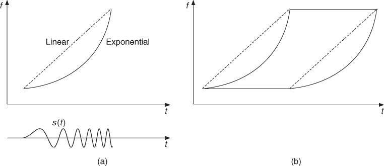
Design 1 As an example, a linear chirp signal is a sine wave with linearly increasing frequency and has the property of having a time delay proportional to its frequency. A mathematical definition of a linear chirp signal starting from frequency zero and going to frequency f1 during time t1 is given by
7.44 ![]()
Sampling of this chirp signal yields the coefficients for an FIR filter. Time-frequency representations of a linear and an exponential chirp signal are shown in Figure 7.22a.
Figure 7.22 Time-frequency representations: (a) linear/exponential chirp signal and (b) time-frequency warping for the linear/exponential chirp.
Design 2 It is also possible to numerically approximate a chirp by integrating an arbitrary frequency function of time. In this case the MATLAB function cumsum can be used to calculate the phase ![]() as the integral of the time-dependent frequency f(t). A linear chirp with 300 samples can be computed by the MATLAB instructions:
as the integral of the time-dependent frequency f(t). A linear chirp with 300 samples can be computed by the MATLAB instructions:
n = 300;
x = (1:n)/n;
f0 = 50;
f1 = 4000;
freq = 2*pi * (f0+(f1-f0)*x) / 44100;
fir = (sin(cumsum(freq)))’;
and an exponential chirp by
n = 300;
x = (1:n)/n;
f0 = 50;
f1 = 4000;
rap = f1/f0;
freq = (2*pi*f0/44100) * (rap.∧x);
fir = (sin(cumsum(freq)))’;
Any other frequency function f(t) can be used for the calculation of freq.
Design 3 Nevertheless these chirp signals deliver the frequency as a function of time delay. We would be more likely to define the time delay as a function of frequency. This is only possible with the previous technique if the function is monotonous. Thus in a more general case we can use the phase information of an FFT as an indication of the time delay corresponding to a frequency bin: the phase of a delayed signal x(n − M), which has a discrete Fourier transform ![]() with k = 0, 1, …, N/2, is
with k = 0, 1, …, N/2, is ![]() , where M is the delay in samples, k is the number of the frequency bin and N is the length of the FFT.
, where M is the delay in samples, k is the number of the frequency bin and N is the length of the FFT.
A variable delay for each frequency bin can be achieved by replacing the fixed value M (the delay of each frequency bin) by a function M(k), which leads to ![]() . For example, a linearly increasing time delay for each frequency bin is given by
. For example, a linearly increasing time delay for each frequency bin is given by ![]() with k = 0, 1, …, N/2 − 1. The derivation of the FIR coefficients can be achieved by performing an IFFT of the positive part of the spectrum and then taking the real part of the resulting complex-valued coefficients. With this technique a linear chirp signal centered around the middle of the window can be computed by the following MATLAB instructions:
with k = 0, 1, …, N/2 − 1. The derivation of the FIR coefficients can be achieved by performing an IFFT of the positive part of the spectrum and then taking the real part of the resulting complex-valued coefficients. With this technique a linear chirp signal centered around the middle of the window can be computed by the following MATLAB instructions:
M = 300;
WLen = 1024;
mask = [1; 2*ones(WLen/2-1,1); 1 ; zeros(WLen/2-1,1)];
fs = M*(0:WLen/2)’ / WLen; % linear increasing delay
teta = [-2*pi*fs.*(0:WLen/2)’/WLen ; zeros(WLen/2-1,1)];
f2 = exp(i*teta);
fir = fftshift(real(ifft(f2.*mask)));
It should be noted that this technique can produce time aliasing. The length of the FIR filter will be greater than M. A proper choice of N is needed, for example N > 2M.
Design 4 A final technique is to draw an arbitrary curve on a time-frequency representation, which is an invalid image, and then resynthesize a signal by forcing a reconstruction, for example, by using a summation of gaborets. Then we can use this reconstructed signal as the impulse response of the FIR filter. If the curve displays the dispersion of a filter, we get a dispersive filter.
In conclusion, we can say that dispersion, which is a filtering operation, can be perceived as a delay operation. This leads to a warping of the time-frequency representation, where each horizontal line of this representation is delayed according to the dispersion curve (see Figure 7.22b).
7.4.3 Time Stretching
Time-frequency scaling is one of the most interesting and difficult tasks that can be assigned to time-frequency representations: changing the time scale independently of the “frequency content.” For example, one can change the rhythm of a song without changing its pitch, or conversely transpose a song without any time change. Time stretching is not a problem that can be stated outside of the perception: we know, for example, that a sum of two sinusoids is equivalent to a product of a carrier and a modulator. Should time stretching of this signal still be a sum of two sinusoids or the same carrier with a lower modulation? This leads us to the perception of tremolo tones or vibrato tones. One generally agrees that tremolos and vibratos under 10 Hz are perceived as such and those over are perceived as a sum of sinusoids. Another example is the exponential decay of sounds produced by percussive gesture (percussions, plucked strings, etc.): should the time-scaled version of such a sound have a natural exponential decay? When time scaling without modeling such aspects, the decay is stretched too, so the exponential decay is modified, potentially resulting in non-physically realistic sounds. A last example is voice (sung or spoken): the perception of some consonants is modified into others when the sound is time scaled, highlighting the fact that it can be interesting to refine such models by modeling the sound content and using non-linear or adaptive processing. Right now, we explain straight time stretching with time-frequency representations and constant control parameters.
One technique has already been evaluated in the time domain (see PSOLA in Section 6.3.3). Here we will deal with another technique in the time-frequency domain using the phase vocoder implementations of Section 7.3. There are two implementations for time-frequency scaling by the “traditional” phase vocoder. Historically, the first one uses a bank of oscillators, whose amplitudes and frequencies vary over time. If we can manage to model a sound by the sum of sinusoids, time stretching and pitch shifting can be performed by expanding the amplitude and frequency functions. The second implementation uses the sliding Fourier transform as the model for resynthesis: if we can manage to spread the image of a sliding FFT over time and calculate new phases, then we can reconstruct a new sound with the help of inverse FFTs. Both of these techniques rely on phase interpolation, which need an unwrapping algorithm at the analysis stage, or equivalently an instantaneous frequency calculation, as introduced in Section 7.3.5.
The time-stretching algorithm mainly consists of providing a synthesis grid which is different from the analysis grid, and to find a way to reconstruct a signal from the values on this grid. Though it is possible to use any stretching factor, we will here only deal with the case where we use an integer both for the analysis hop size Ra, and for the synthesis hop size Rs.
As seen in Section 7.3, changing the values and their coordinates on a time-frequency representation is generally not a valid operation, in the sense that the resulting representation is not the sliding Fourier transform of a real signal. However, it is always possible to force the reconstruction of a sound from an arbitrary image, but the time-frequency representation of the signal issued from this forced synthesis will be different from what was expected. The goal of a good transformation algorithm is to find a strategy that preserves the time-stretching aspect without introducing too many artifacts.
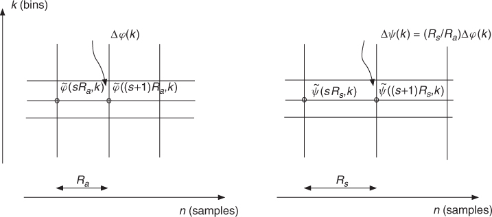
The classical way of using a phase vocoder for time stretching is to keep the magnitude unchanged and to modify the phase in such a way that the instantaneous frequencies are preserved. Providing that the grid is enlarged from an analysis hop size Ra to a synthesis hop size Rs, this means that the new phase values must satisfy ![]() (see Figure 7.23). Once the grid is filled with these values one can reconstruct a signal using either the filter-bank approach or the block-by-block IFFT approach.
(see Figure 7.23). Once the grid is filled with these values one can reconstruct a signal using either the filter-bank approach or the block-by-block IFFT approach.
Figure 7.23 Time-stretching principle: analysis with hop size Ra gives the time-frequency grid shown in the left part, where ![]() denotes the phase difference between the unwrapped phases. The synthesis is performed from the modified time-frequency grid with hop size Rs and the phase difference
denotes the phase difference between the unwrapped phases. The synthesis is performed from the modified time-frequency grid with hop size Rs and the phase difference ![]() , which is illustrated in the right part.
, which is illustrated in the right part.
Filter-bank Approach (Sum of Sinusoids)
In the FFT analysis/sum of sinusoids synthesis approach, we calculate the instantaneous frequency for each bin and integrate the corresponding phase increment in order to reconstruct a signal as the weighted sum of cosines of the phases. However, here the hop size for the resynthesis is different from the analysis. Therefore the following steps are necessary:
1. Calculate the phase increment per sample by dψ(k) = Δφ(k)/Ra.
2.For the output samples of the resynthesis integrate this value according to ![]() .
.
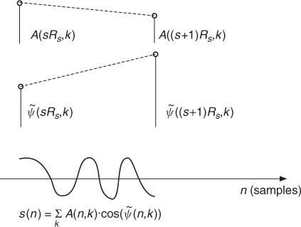
3. Sum the intermediate signals which yields ![]() (see Figure 7.24).
(see Figure 7.24).
A complete MATLAB program for time stretching is given by M-file 7.8.
M-file 7.8 (VX_tstretch_bank.m)
% VX_tstretch_bank.m [DAFXbook, 2nd ed., chapter 7]
%===== This program performs time stretching
%===== using the oscillator bank approach
clear; clf
%----- user data -----
n1 = 256; % analysis step increment [samples]
n2 = 512; % synthesis step increment [samples]
s_win = 2048; % analysis window length [samples]
[DAFx_in, FS] = wavread(‘la.wav’);
%----- initialize windows, arrays, etc -----
tstretch_ratio = n2/n1
w1 = hanning(s_win, ‘periodic’); % analysis window
w2 = w1; % synthesis window
L = length(DAFx_in);
DAFx_in = [zeros(s_win, 1); DAFx_in; ...
zeros(s_win-mod(L,n1),1)] / max(abs(DAFx_in)); % 0-pad & normalize
DAFx_out = zeros(s_win+ceil(length(DAFx_in)*tstretch_ratio),1);
grain = zeros(s_win,1);
ll = s_win/2;
omega = 2*pi*n1*[0:ll-1]'/s_win;
phi0 = zeros(ll,1);
r0 = zeros(ll,1);
psi = zeros(ll,1);
res = zeros(n2,1);
%UUUUUUUUUUUUUUUUUUUUUUUUUUUUUUUUUUUUUUU
pin = 0;
pout = 0;
pend = length(DAFx_in)-s_win;
while pin<pend
grain = DAFx_in(pin+1:pin+s_win).* w1;
%===========================================
fc = fft(fftshift(grain));
f = fc(1:ll);
r = abs(f);
phi = angle(f);
%----- calculate phase increment per block -----
delta_phi = omega + princarg(phi-phi0-omega);
%----- calculate phase & mag increments per sample -----
delta_r = (r-r0) / n2; % for synthesis
delta_psi = delta_phi / n1; % derived from analysis
%----- computing output samples for current block -----
for k=1:n2
r0 = r0 + delta_r;
psi = psi + delta_psi;
res(k) = r0'*cos(psi);
end
%----- values for processing next block -----
phi0 = phi;
r0 = r;
psi = princarg(psi);
% ===========================================
% DAFx_out(pout+1:pout+n2) = DAFx_out(pout+1:pout+n2)+res;
DAFx_out(pout+1:pout+n2) = res;
pin = pin + n1;
pout = pout + n2;
end
%UUUUUUUUUUUUUUUUUUUUUUUUUUUUUUUUUUUUUUU
%----- listening and saving the output -----
% DAFx_in = DAFx_in(s_win+1:s_win+L);
DAFx_out=DAFx_out(s_win/2+n1+1:length(DAFx_out))/max(abs(DAFx_out));
soundsc(DAFx_out, FS);
wavwrite(DAFx_out, FS, ‘la_tstretch_bank.wav’);
Figure 7.24 Calculation of time-frequency samples. Given the values of A and ![]() on the representation grid, we can perform linear interpolation with a hop size between two successive values on the grid. The reconstruction is achieved by a summation of weighted cosines.
on the representation grid, we can perform linear interpolation with a hop size between two successive values on the grid. The reconstruction is achieved by a summation of weighted cosines.
This program first extracts a series of sound segments called grains. For each grain the FFT is computed to yield a magnitude and phase representation every n1 samples (n1 is the analysis hop size Ra). It then calculates a sequence of n2 samples (n2 is the synthesis hop size Rs) of the output signal by interpolating the values of r and calculating the phase psi in such a way that the instantaneous frequency derived from psi is equal to the one derived from phi. The unwrapping of the phase is then done by calculating (phi-phi0-omega), putting it in the range [−π, π] and again adding omega. A phase increment per sample d_psi is calculated from delta_phi/n1. The calculation of the magnitude and phase at the resynthesis is done in the loop for k=1:n2 where r and psi are incremented by d_r and d_psi. The program uses the vector facility of MATLAB to calculate the sum of the cosine of the angles weighted by magnitude in one step. This gives a buffer res of n2 output samples which will be inserted into the DAFx_out signal.
Block-by-block Approach (FFT/IFFT)
Here we follow the FFT/IFFT implementation used in Section 7.3, but the hop size for resynthesis is different from the analysis. So we have to calculate new phase values in order to preserve the instantaneous frequencies for each bin. This is again done by calculating an unwrapped phase difference for each frequency bin, which is proportional to ![]() . We also have to take care of some implementation details, such as the fact that the period of the window has to be equal to the length of the FFT (this is not the case for the standard MATLAB functions). The synthesis hop size should at least allow a minimal overlap of windows, or should be a submultiple of it. It is suggested to use overlap values of at least 75% (i.e., Ra ≤ n1/4). The following M-file 7.9 demonstrates the block-by-block FFT/IFFT implementation.
. We also have to take care of some implementation details, such as the fact that the period of the window has to be equal to the length of the FFT (this is not the case for the standard MATLAB functions). The synthesis hop size should at least allow a minimal overlap of windows, or should be a submultiple of it. It is suggested to use overlap values of at least 75% (i.e., Ra ≤ n1/4). The following M-file 7.9 demonstrates the block-by-block FFT/IFFT implementation.
M-file 7.9 (VX_tstretch_real_pv.m)
% VX_tstretch_real_pv.m [DAFXbook, 2nd ed., chapter 7]
%===== This program performs time stretching
%===== using the FFT-IFFT approach, for real ratios
clear; clf
%----- user data -----
n1 = 200; % analysis step [samples]
n2 = 512; % synthesis step ([samples]
s_win = 2048; % analysis window length [samples]
[DAFx_in,FS] = wavread(‘la.wav’);
%----- initialize windows, arrays, etc -----
tstretch_ratio = n2/n1
w1 = hanning(s_win, ‘periodic’); % analysis window
w2 = w1; % synthesis window
L = length(DAFx_in);
DAFx_in = [zeros(s_win, 1); DAFx_in; ...
zeros(s_win-mod(L,n1),1)] / max(abs(DAFx_in));
DAFx_out = zeros(s_win+ceil(length(DAFx_in)*tstretch_ratio),1);
omega = 2*pi*n1*[0:s_win-1]'/s_win;
phi0 = zeros(s_win,1);
psi = zeros(s_win,1);
tic
%UUUUUUUUUUUUUUUUUUUUUUUUUUUUUUUUUUUUUUU
pin = 0;
pout = 0;
pend = length(DAFx_in)-s_win;
while pin<pend
grain = DAFx_in(pin+1:pin+s_win).* w1;
%===========================================
f = fft(fftshift(grain));
r = abs(f);
phi = angle(f);
%---- computing input phase increment ----
delta_phi = omega + princarg(phi-phi0-omega);
%---- computing output phase increment ----
psi = princarg(psi+delta_phi*tstretch_ratio);
%---- comouting synthesis Fourier transform & grain ----
ft = (r.* exp(i*psi));
grain = fftshift(real(ifft(ft))).*w2;
% plot(grain);drawnow;
% ===========================================
DAFx_out(pout+1:pout+s_win) = ...
DAFx_out(pout+1:pout+s_win) + grain;
%----- for next block -----
phi0 = phi;
pin = pin + n1;
pout = pout + n2;
end
%UUUUUUUUUUUUUUUUUUUUUUUUUUUUUUUUUUUUUUU
toc
%----- listening and saving the output -----
%DAFx_in = DAFx_in(s_win+1:s_win+L);
DAFx_out = DAFx_out(s_win+1:length(DAFx_out))/max(abs(DAFx_out));
soundsc(DAFx_out, FS);
wavwrite(DAFx_out, FS, ‘la_tstretch_noint_pv.wav’);
This program is much faster than the preceding one. It extracts grains of the input signal by windowing the original signal DAFx_in, makes a transformation of these grains and overlap-adds these transformed grains to get a sound DAFx_out. The transformation consists of performing the FFT of the grain and computing the magnitude and phase representation r and phi. The unwrapping of the phase is then done by calculating (phi-phi0-omega), putting it in the range [−π, π] and again adding omega. The calculation of the phase psi of the transformed grain is then achieved by adding the phase increment delta_phi multiplied by the stretching factor ral to the previous unwrapped phase value. As seen before, this is equivalent to keeping the same instantaneous frequency for the synthesis as is calculated for the analysis. The new output grain is then calculated by an inverse FFT, windowed again and overlap-added to the output signal.
Hints and drawbacks As we have noticed, phase vocoding can produce artifacts. It is important to know them in order to face them.
1. Changing the phases before the IFFT is equivalent to using an all pass filter whose Fourier transform contains the phase correction that is being applied. If we do not use a window for the resynthesis, we can ensure the circular convolution aspect of this filtering operation. We will have discontinuities at the edges of the signal buffer. So it is necessary to use a synthesis window.
2. Nevertheless, even with a resynthesis window (also called tapering window) the circular aspect still remains: the result is the aliased version of an infinite IFFT. A way to counteract this is to choose a zero-padded window for analysis and synthesis.
3. Shape of the window: one must ensure that a perfect reconstruction is given with a ratio ![]() equal to one (no time stretching). If we use the same window for analysis and synthesis, the sum of the square of the windows, regularly spaced at the resynthesis hope size, should be one.
equal to one (no time stretching). If we use the same window for analysis and synthesis, the sum of the square of the windows, regularly spaced at the resynthesis hope size, should be one.
4. For a Hanning window without zero-padding the hop size Rs has to be a divisor of N/4.
5. Hamming and Blackman windows provide smaller side lobes in the Fourier transform. However, they have the inconvenience of being non-zero at the edges, so that no tapering is done by using these windows alone. The resynthesis hop size should be a divisor of N/8.
6. Truncated Gaussian windows, which are good candidates, provide a sum that always has oscillations, but which can be below the level of perception.
Phase dispersion An important problem is the difference of phase unwrapping between different bins, which is not solved by the algorithms we presented: the unwrapping algorithm of the analysis gives a phase that is equal to the measured phase modulo 2π. So the unwrapped phase is equal to the measured phase plus a term that is a multiple of 2π. This second term is not the same for every bin. Because of the multiplication by the time-stretching ratio, there is a dispersion of the phases. One cannot even ensure that two identical successive sounds will be treated in the same way. This is in fact the main drawback of the phase vocoder and its removal is treated in several publications [QM98, Fer99, LD99a, Lar03, Röb03, Röb10].
Phase-locked Vocoder
One of the most successful approaches to reduce the phase dispersion was proposed in [LD99a]. If we consider the processed sound to be mostly composed of quasi-sinusoidal components, then we can approximate its spectrum as the sum of the complex convolution of each of those components by the analysis window transform (this will be further explained in the spectral processing chapter). When we transform the sound, for instance time stretching it, the phase of those quasi-sinusoidal components has to propagate accordingly. What is really interesting here is that for each sinusoid the effect of the phase propagation on the spectrum is nothing more than a constant phase rotation of all the spectral bins affected by it. This method is referred to as phase-locked vocoder, since the phase of each spectral bin is locked to the phase of one spectral peak.
Starting from the previous M-file, we need to add the following steps to the processing loop:
1. Find spectral peaks. A good tradeoff is to find local maxima in a predefined frequency range, for instance considering two bins around each candidate. This helps to minimize spurious peaks as well as to reduce the likelihood of identifying analysis window transform side-lobes as spectral peaks.
2. Connect current peaks to previous frame peaks. The simplest approach is to choose the closest peak in frequency.
3. Propagate peaks. A simple but usually effective strategy is to consider that peaks evolve linearly in frequency.
4. Rotate equally all bins assigned to each spectral peak. The assignment can be performed by segmenting the spectrum into frequency regions delimited by the middle bin between consecutive peaks. An alternative is to set the segment boundaries to the bin with minimum amplitude between consecutive peaks.
Furthermore, the code can be optimized taking into account that the spectrum of a real signal is hermitic, so that we do only need to process the first half of the spectrum. A complete MATLAB program for time stretching using the phase-locked vocoder is given by M-file 7.10.
M-file 7.10 (VX_tstretch_real_pv_phaselocked.m)
% VX_tstretch_real_pv_phaselocked.m [DAFXbook, 2nd ed., chapter 7]
%===== this program performs real ratio time stretching using the
%===== FFT-IFFT approach, applying spectral peak phase-locking
clear; clf
%----- user data -----
n1 = 256; % analysis step [samples]
n2 = 300; % synthesis step ([samples]
s_win = 2048; % analysis window length [samples]
[DAFx_in,FS] = wavread(‘la.wav’);
%----- initialize windows, arrays, etc -----
tstretch_ratio = n2/n1
hs_win = s_win/2;
w1 = hanning(s_win, ‘periodic’); % analysis window
w2 = w1; % synthesis window
L = length(DAFx_in);
DAFx_in = [zeros(s_win, 1); DAFx_in; ...
zeros(s_win-mod(L,n1),1)] / max(abs(DAFx_in));
DAFx_out = zeros(s_win+ceil(length(DAFx_in)*tstretch_ratio),1);
omega = 2*pi*n1*[0:hs_win]'/s_win;
phi0 = zeros(hs_win+1,1);
psi = zeros(hs_win+1,1);
psi2 = psi;
nprevpeaks = 0;
tic
%UUUUUUUUUUUUUUUUUUUUUUUUUUUUUUUUUUUUUUU
pin = 0;
pout = 0;
pend = length(DAFx_in) - s_win;
while pin<pend
grain = DAFx_in(pin+1:pin+s_win).* w1;
%===========================================
f = fft(fftshift(grain));
%---- optimization: only process the first 1/2 of the spectrum
f = f(1:hs_win+1);
r = abs(f);
phi = angle(f);
%---- find spectral peaks (local maxima) ----
peak_loc = zeros(hs_win+1,1);
npeaks = 0;
for b=3:hs_win-1
if ( r(b)>r(b-1) && r(b)>r(b-2) && r(b)>r(b+1) && r(b)>r(b+2) )
npeaks = npeaks+1;
peak_loc(npeaks) = b;
b = b + 3;
end
end
%---- propagate peak phases and compute spectral bin phases
if (pin==0) % init
psi = phi;
elseif (npeaks>0 && nprevpeaks>0)
prev_p = 1;
for p=1:npeaks
p2 = peak_loc(p);
%---- connect current peak to the previous closest peak
while (prev_p < nprevpeaks && abs(p2-prev_peak_loc(prev_p+1)) ...
< abs(p2-prev_peak_loc(prev_p)))
prev_p = prev_p+1;
end
p1 = prev_peak_loc(prev_p);
%---- propagate peak's phase assuming linear frequency
%---- variation between connected peaks p1 and p2
avg_p = (p1 + p2)*.5;
pomega = 2*pi*n1*(avg_p-1.)/s_win;
% N.B.: avg_p is a 1-based indexing spectral bin
peak_delta_phi = pomega + princarg(phi(p2)-phi0(p1)-pomega);
peak_target_phase = princarg(psi(p1) + peak_delta_phi*tstretch_ratio);
peak_phase_rotation = princarg(peak_target_phase-phi(p2));
%---- rotate phases of all bins around the current peak
if (npeaks==1)
bin1 = 1; bin2 = hs_win+1;
elseif (p==1)
bin1 = 1; bin2 = hs_win+1;
elseif (p==npeaks)
bin1 = round((peak_loc(p-1)+p2)*.5);
bin2 = hs_win+1;
else
bin1 = round((peak_loc(p-1)+p2)*.5)+1;
bin2 = round((peak_loc(p+1)+p2)*.5);
end
psi2(bin1:bin2) = princarg(phi(bin1:bin2) + peak_phase_rotation);
end
psi = psi2;
else
delta_phi = omega + princarg(phi-phi0-omega);
psi = princarg(psi+delta_phi*tstretch_ratio);
end
ft = (r.* exp(i*psi));
%---- reconstruct whole spectrum (it is hermitic!)
ft = [ ft(1:hs_win+1) ; conj(ft(hs_win:-1:2)) ];
grain = fftshift(real(ifft(ft))).*w2;
% plot(grain);drawnow;
% ===========================================
DAFx_out(pout+1:pout+s_win) = ...
DAFx_out(pout+1:pout+s_win) + grain;
%---- store values for next frame ----
phi0 = phi;
prev_peak_loc = peak_loc;
nprevpeaks = npeaks;
pin = pin + n1;
pout = pout + n2;
end
%UUUUUUUUUUUUUUUUUUUUUUUUUUUUUUUUUUUUUUU
toc
%----- listening and saving the output -----
%DAFx_in = DAFx_in(s_win+1:s_win+L);
DAFx_out = DAFx_out(s_win+1:length(DAFx_out))/max(abs(DAFx_out));
soundsc(DAFx_out, FS);
wavwrite(DAFx_out, FS, ‘la_tstretch_noint_pv_phaselocked.wav’);
Integer Ratio Time Stretching
When the time-stretching ratio is an integer (e.g., time stretching by 200%, 300%), the unwrapping is no longer necessary in the algorithm, because the 2π modulo relation is still preserved when the phase is multiplied by an integer. The key point here is that we can make a direct multiplication of the analysis phase to get the phase for synthesis. So in this case it is more obvious and elegant to use the following algorithm, given by M-file 7.11.
M-file 7.11 (VX_tstretch_int_pv.m)
% VX_tstretch_int_pv.m [DAFXbook, 2nd ed., chapter 7]
%===== This program performs integer ratio time stretching
%===== using the FFT-IFFT approach
clear; clf
%----- user data -----
n1 = 64; % analysis step [samples]
n2 = 512; % synthesis step ([samples]
s_win = 2048; % analysis window length [samples]
[DAFx_in,FS] = wavread(‘la.wav’);
%----- initialize windows, arrays, etc -----
tstretch_ratio = n2/n1
w1 = hanning(s_win, ‘periodic’); % analysis window
w2 = w1; % synthesis window
L = length(DAFx_in);
DAFx_in = [zeros(s_win, 1); DAFx_in; ...
zeros(s_win-mod(L,n1),1)] / max(abs(DAFx_in));
DAFx_out = zeros(s_win+ceil(length(DAFx_in)*tstretch_ratio),1);
omega = 2*pi*n1*[0:s_win-1]'/s_win;
phi0 = zeros(s_win,1);
psi = zeros(s_win,1);
tic
%UUUUUUUUUUUUUUUUUUUUUUUUUUUUUUUUUUUUUUU
pin = 0;
pout = 0;
pend = length(DAFx_in)-s_win;
while pin<pend
grain = DAFx_in(pin+1:pin+s_win).* w1;
%===========================================
f = fft(fftshift(grain));
r = abs(f);
phi = angle(f);
ft = (r.* exp(i*tstretch_ratio*phi));
grain = fftshift(real(ifft(ft))).*w2;
% ===========================================
DAFx_out(pout+1:pout+s_win) = ...
DAFx_out(pout+1:pout+s_win) + grain;
pin = pin + n1;
pout = pout + n2;
end
%UUUUUUUUUUUUUUUUUUUUUUUUUUUUUUUUUUUUUUU
toc
%----- listening and saving the output -----
% DAFx_in = DAFx_in(s_win+1:s_win+L);
DAFx_out = DAFx_out(s_win+1:length(DAFx_out))/max(abs(DAFx_out));
soundsc(DAFx_out, FS);
wavwrite(DAFx_out, FS, ‘la_stretch_int_pv.wav’);
7.4.4 Pitch Shifting
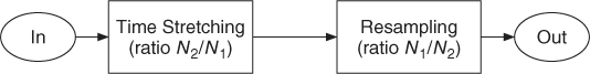
Pitch shifting is different from frequency shifting: a frequency shift is an addition to every frequency (i.e., the magnitude spectrum is shifted), while pitch shifting is the multiplication of every frequency by a transposition factor (i.e., the magnitude spectrum is scaled). Pitch shifting can be directly linked to time stretching. Resampling a time-stretched signal with the inverse of the time-stretching ratio performs pitch shifting and going back to the initial duration of the signal (see Figure 7.25). There are, however, alternative solutions which allow the direct calculation of a pitch-shifted version of a sound.
Figure 7.25 Resampling of a time-stretching algorithm.
Filter-bank Approach (Sum of Sinusoids)
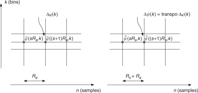
In the time-stretching algorithm using the sum of sinusoids (see Section 7.3) we have an evaluation of instantaneous frequencies. As a matter of fact transposing all the instantaneous frequencies can lead to an efficient pitch-shifting algorithm. Therefore the following steps have to be performed (see Figure 7.26):
1. Calculate the phase increment per sample by dφ(k) = Δφ(k)/Ra.
2. Multiply the phase increment by the transposition factor transpo and integrate the modified phase increment according to ![]() transpo · Δφ(k)/Ra.
transpo · Δφ(k)/Ra.
3. Calculate the sum of sinusoids: when the transposition factor is greater than one, keep only frequencies under the Nyquist frequency bin N/2. This can be done by taking only the N/(2*transpo) frequency bins.
Figure 7.26 Pitch shifting with the filter-bank approach: the analysis gives the time-frequency grid with analysis hop size Ra. For the synthesis the hop size is set to Rs = Ra and the phase difference is calculated according to Δψ(k) = transpo Δφ(k).
The following M-file 7.12 is similar to the program given by M-file 7.8 with the exception of a few lines: the definition of the hop size and the resynthesis phase increment have been changed.
M-file 7.12 (VX_pitch_bank.m)
% VX_pitch_bank.m [DAFXbook, 2nd ed., chapter 7]
%===== This program performs pitch shifting
%===== using the oscillator bank approach
clear; clf
%----- user data -----
n1 = 512; % analysis step [samples]
pit_ratio = 1.2 % pitch-shifting ratio
s_win = 2048; % analysis window length [samples]
[DAFx_in,FS] = wavread(‘la.wav’);
%----- initialize windows, arrays, etc -----
w1 = hanning(s_win, ‘periodic’); % analysis window
w2 = w1; % synthesis window
L = length(DAFx_in);
DAFx_in = [zeros(s_win, 1); DAFx_in; ...
zeros(s_win-mod(L,n1),1)] / max(abs(DAFx_in));
DAFx_out = zeros(length(DAFx_in),1);
grain = zeros(s_win,1);
hs_win = s_win/2;
omega = 2*pi*n1*[0:hs_win-1]'/s_win;
phi0 = zeros(hs_win,1);
r0 = zeros(hs_win,1);
psi = phi0;
res = zeros(n1,1);
tic
%UUUUUUUUUUUUUUUUUUUUUUUUUUUUUUUUUUUUUUU
pin = 0;
pout = 0;
pend = length(DAFx_in)-s_win;
while pin<pend
grain = DAFx_in(pin+1:pin+s_win).* w1;
%===========================================
fc = fft(fftshift(grain));
f = fc(1:hs_win);
r = abs(f);
phi = angle(f);
%---- compute phase & mangitude increments ----
delta_phi = omega + princarg(phi-phi0-omega);
delta_r = (r-r0)/n1;
delta_psi = pit_ratio*delta_phi/n1;
%---- compute output buffer ----
for k=1:n1
r0 = r0 + delta_r;
psi = psi + delta_psi;
res(k) = r0' * cos(psi);
end
%---- store for next block ----
phi0 = phi;
r0 = r;
psi = princarg(psi);
% plot(res);pause;
% ===========================================
DAFx_out(pout+1:pout+n1) = DAFx_out(pout+1:pout+n1) + res;
pin = pin + n1;
pout = pout + n1;
end
%UUUUUUUUUUUUUUUUUUUUUUUUUUUUUUUUUUUUUUU
toc
%----- listening and saving the output -----
% DAFx_in = DAFx_in(s_win+1:s_win+L);
DAFx_out = DAFx_out(hs_win+n1+1:hs_win+n1+L) / max(abs(DAFx_out));
soundsc(DAFx_out, FS);
wavwrite(DAFx_out, FS, ‘la_pitch_bank.wav’);
The program is derived from the time-stretching program using the oscillator-bank approach in a straightforward way: this time the hop size for analysis and synthesis are the same, and a pitch transpose argument pit must be defined. This argument will be multiplied by the phase increment delta_phi/n1 derived from the analysis to get the phase increment d_psi in the calculation loop. This means of course that we consider the pitch transposition as fixed in this program, but easy changes may be done to make it vary with time.
Block-by-block Approach (FFT/IFFT)
The regular way to deal with pitch shifting using this technique is first to resample the whole output once computed, but this can alternatively be done by resampling the result of every IFFT and overlapping with a hop size equal to the analysis one (see Figure 7.27). Providing that Rs is a divider of N (FFT length), which is quite a natural way for time stretching (to ensure that the sum of the square of windows is equal to one), one can resample each IFFT result to a length of ![]() and overlap with a hop size of Ra. Another method of resampling is to use the property of the inverse FFT: if Ra < Rs, we can take an IFFT of length
and overlap with a hop size of Ra. Another method of resampling is to use the property of the inverse FFT: if Ra < Rs, we can take an IFFT of length ![]() by taking only the first bins of the initial FFT. If Ra > Rs, we can zero pad the FFT, before the IFFT is performed. In each of these cases the result is a resampled grain of length
by taking only the first bins of the initial FFT. If Ra > Rs, we can zero pad the FFT, before the IFFT is performed. In each of these cases the result is a resampled grain of length ![]() .
.
Figure 7.27 Pitch shifting with integrated resampling: for each grain time stretching and resampling are performed. An overlap-add procedure delivers the output signal.
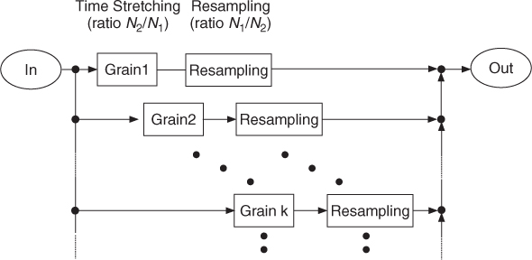
The following M-file 7.13 implements pitch shifting with integrated resampling according to Figure 7.27. The M-file is similar to the program given by M-file 7.11, except for the definition of the hop sizes and the calculation for the interpolation.
M-file 7.13 (VX_pitch_pv.m)
% VX_pitch_pv.m [DAFXbook, 2nd ed., chapter 7]
%===== This program performs pitch shifting
%===== using the FFT/IFFT approach
clear; clf
%----- user data -----
n2 = 512; % synthesis step [samples]
pit_ratio = 1.2 % pitch-shifting ratio
s_win = 2048; % analysis window length [samples]
[DAFx_in,FS] = wavread(‘flute2’);
%----- initialize windows, arrays, etc -----
n1 = round(n2 / pit_ratio); % analysis step [samples]
tstretch_ratio = n2/n1;
w1 = hanning(s_win, ‘periodic’); % analysis window
w2 = w1; % synthesis window
L = length(DAFx_in);
DAFx_in = [zeros(s_win, 1); DAFx_in; ...
zeros(s_win-mod(L,n1),1)] / max(abs(DAFx_in));
DAFx_out = zeros(length(DAFx_in),1);
omega = 2*pi*n1*[0:hs_win-1]'/s_win;
phi0 = zeros(s_win,1);
psi = zeros(s_win,1);
%----- for linear interpolation of a grain of length s_win -----
lx = floor(s_win*n1/n2);
x = 1 + (0:lx-1)'*s_win/lx;
ix = floor(x);
ix1 = ix + 1;
dx = x - ix;
dx1 = 1 - dx;
tic
%UUUUUUUUUUUUUUUUUUUUUUUUUUUUUUUUUUUUUUU
pin = 0;
pout = 0;
pend = length(DAFx_in)-s_win;
while pin<pend
grain = DAFx_in(pin+1:pin+s_win).* w1;
%===========================================
f = fft(fftshift(grain));
r = abs(f);
phi = angle(f);
%---- computing phase increment ----
delta_phi = omega + princarg(phi-phi0-omega);
phi0 = phi;
psi = princarg(psi+delta_phi*tstretch_ratio);
%---- synthesizing time scaled grain ----
ft = (r.* exp(i*psi));
grain = fftshift(real(ifft(ft))).*w2;
%----- interpolating grain -----
grain2 = [grain;0];
grain3 = grain2(ix).*dx1+grain2(ix1).*dx;
% plot(grain);drawnow;
% ===========================================
DAFx_out(pout+1:pout+lx) = DAFx_out(pout+1:pout+lx) + grain3;
pin = pin + n1;
pout = pout + n1;
end
%UUUUUUUUUUUUUUUUUUUUUUUUUUUUUUUUUUUUUUU
toc
%----- listening and saving the output -----
% DAFx_in = DAFx_in(s_win+1:s_win+L);
DAFx_out = DAFx_out(s_win+1:s_win+L) / max(abs(DAFx_out));
soundsc(DAFx_out, FS);
wavwrite(DAFx_out, FS, ‘flute2_pitch_pv.wav’);
This program is adapted from the time-stretching program using the FFT/IFFT approach. Here the grain is linearly interpolated before the reconstruction. The length of the interpolated grain is now lx and will be overlapped and added with a hop size of n1 identical to the analysis hop size. In order to speed up the calculation of the interpolation, four vectors of length lx are precalculated outside the main loop, which give the necessary parameters for the interpolation (ix, ix1, dx and dx1). As stated previously, the linear interpolation is not necessarily the best one, and will surely produce some foldover when the pitch-shifting factor is greater than one. Other interpolation schemes can be inserted instead. Further pitch-shifting techniques can be found in [QM98, Lar98, LD99b].
7.4.5 Stable/transient Components Separation
This effect extracts “stable components” from a signal by selecting only points of the time-frequency representation that are considered as “stable in frequency” and eliminating all the other grains. Basic ideas can be found in [SL94]. From a musical point of view, one would think about getting only sine waves, and leave aside all the transient signals. However, this is not so: even with pure noise, the time-frequency analysis reveals some zones where we can have stable components. A pulse will also give an analysis where the instantaneous frequencies are the ones of the analyzing system and are very stable. Nevertheless this idea of separating a sound into two complementary sounds is indeed a musically good one. The result can be thought of as an “etherization” of the sound for the stable one, and a “fractalization” for the transient one.
The algorithm for components separation is based on instantaneous frequency computation. The increment of the phase per sample for frequency bin k can be derived as
We will now sort out those points of a given FFT that give
where df is a preset value. From (7.45) and (7.46) we can derive the condition
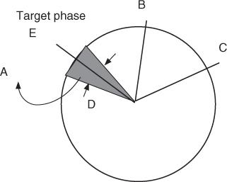
From a geometrical point of view we can say that the value ![]() should be in an angle dfRa around the expected target value
should be in an angle dfRa around the expected target value ![]() , as shown in Figure 7.28.
, as shown in Figure 7.28.
Figure 7.28 Evaluation of stable/unstable grains.
It is important to note that the instantaneous frequencies may be out of the range of frequencies of the bin itself. The reconstruction performed by the inverse FFT takes only bins that follow this condition. In other words, only gaborets that follow the “frequency stability over time” condition are kept during the reconstruction. The following M-file 7.14 follows this guideline.
M-file 7.14 (VX_stable.m)
% VX_stable.m [DAFXbook, 2nd ed., chapter 7]
%===== this program extracts the stable components of a signal
clear; clf
%----- user data -----
test = 0.4
n1 = 256; % analysis step [samples]
n2 = n1; % synthesis step [samples]
s_win = 2048; % analysis window length [samples]
[DAFx_in,FS] = wavread(‘redwheel.wav’);
%----- initialize windows, arrays, etc -----
w1 = hanning(s_win, ‘periodic’); % analysis window
w2 = w1; % synthesis window
L = length(DAFx_in);
DAFx_in = [zeros(s_win, 1); DAFx_in; ...
zeros(s_win-mod(L,n1),1)] / max(abs(DAFx_in));
DAFx_out = zeros(length(DAFx_in),1);
devcent = 2*pi*n1/s_win;
vtest = test * devcent
grain = zeros(s_win,1);
theta1 = zeros(s_win,1);
theta2 = zeros(s_win,1);
tic
%UUUUUUUUUUUUUUUUUUUUUUUUUUUUUUUUUUUUUUU
pin = 0;
pout = 0;
pend = length(DAFx_in)-s_win;
while pin<pend
grain = DAFx_in(pin+1:pin+s_win).* w1;
%===========================================
f = fft(fftshift(grain));
theta = angle(f);
dev = princarg(theta - 2*theta1 + theta2);
% plot(dev);drawnow;
%---- set to 0 magnitude values below ‘test’ threshold
ft = f.*(abs(dev) < vtest);
grain = fftshift(real(ifft(ft))).*w2;
theta2 = theta1;
theta1 = theta;
% ===========================================
DAFx_out(pout+1:pout+s_win) = ...
DAFx_out(pout+1:pout+s_win) + grain;
pin = pin + n1;
pout = pout + n2;
end
%UUUUUUUUUUUUUUUUUUUUUUUUUUUUUUUUUUUUUUU
toc
%----- listening and saving the output -----
% DAFx_in = DAFx_in(s_win+1:s_win+L);
DAFx_out = DAFx_out(s_win+1:s_win+L) / max(abs(DAFx_out));
soundsc(DAFx_out, FS);
wavwrite(DAFx_out, FS, ‘redwheel_stable.wav’);
So the algorithm for extraction of stable components performs the following steps:
1. Calculate the instantaneous frequency by making the derivative of the phase along the time axis.
2. Check if this frequency is within its “stable range.”
3. Use the frequency bin or not for the reconstruction.
The value of vtest is particularly important because it determines the level of the selection between stable and unstable bins.
The algorithm for transient components extraction is the same, except that we keep only bins where the condition (7.47) is not satisfied. So only two lines have to be changed according to
test = 2 % new value for test threshold
...
ft = f*(abs(dev)>vtest); % new condition
In order to enhance the unstable grains the value vtest is usually higher for the transient extraction.
7.4.6 Mutation between two sounds
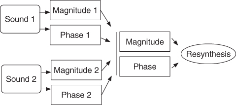
The idea is to calculate an arbitrary time-frequency representation from two original sounds and to reconstruct a sound from it. Some of these spectral mutations (see Figure 7.29) give a flavor of cross-synthesis and morphing, a subject that will be discussed later, but are different from it, because here the effect is only incidental, while in cross-synthesis hybridization of sounds is the primary objective. Further ideas can be found in [PE96]. There are different ways to calculate a new combined magnitude and phase diagram from the values of the original ones. As stated in Section 7.3, an arbitrary image is not valid in the sense that it is not the time-frequency representation of a sound, which means that the result will be musically biased by the resynthesis scheme that we must use. Usually phases and magnitudes are calculated in an independent way, so that many combinations are possible. Not all of them are musically relevant, and the result also depends upon the nature of the sounds that are combined.
Figure 7.29 Basic principle of spectral mutations.
The following M-file 7.15 performs a mutation between two sounds where the magnitude is coming from one sound and the phase from the other. Then only a few lines need to be changed to give different variations.
M-file 7.15 (VX_mutation.m)
% VX_mutation.m [DAFXbook, 2nd ed., chapter 7]
%===== this program performs a mutation between two sounds,
%===== taking the phase of the first one and the modulus
%===== of the second one, and using:
%===== w1 and w2 windows (analysis and synthesis)
%===== WLen is the length of the windows
%===== n1 and n2: steps (in samples) for the analysis and synthesis
clear; clf
%----- user data -----
n1 = 512;
n2 = n1;
WLen = 2048;
w1 = hanningz(WLen);
w2 = w1;
[DAFx_in1,FS] = wavread(‘x1.wav’);
DAFx_in2 = wavread(‘x2.wav’);
%----- initializations -----
L = min(length(DAFx_in1),length(DAFx_in2));
DAFx_in1 = [zeros(WLen, 1); DAFx_in1; ...
zeros(WLen-mod(L,n1),1)] / max(abs(DAFx_in1));
DAFx_in2 = [zeros(WLen, 1); DAFx_in2; ...
zeros(WLen-mod(L,n1),1)] / max(abs(DAFx_in2));
DAFx_out = zeros(length(DAFx_in1),1);
tic
%UUUUUUUUUUUUUUUUUUUUUUUUUUUUUUUUUUUUUUU
pin = 0;
pout = 0;
pend = length(DAFx_in1) - WLen;
while pin<pend
grain1 = DAFx_in1(pin+1:pin+WLen).* w1;
grain2 = DAFx_in2(pin+1:pin+WLen).* w1;
%===========================================
f1 = fft(fftshift(grain1));
r1 = abs(f1);
theta1 = angle(f1);
f2 = fft(fftshift(grain2));
r2 = abs(f2);
theta2 = angle(f2);
%----- the next two lines can be changed according to the effect
r = r1;
theta = theta2;
ft = (r.* exp(i*theta));
grain = fftshift(real(ifft(ft))).*w2;
% ===========================================
DAFx_out(pout+1:pout+WLen) = ...
DAFx_out(pout+1:pout+WLen) + grain;
pin = pin + n1;
pout = pout + n2;
end
%UUUUUUUUUUUUUUUUUUUUUUUUUUUUUUUUUUUUUUU
toc
%----- listening and saving the output -----
%DAFx_in = DAFx_in(WLen+1:WLen+L);
DAFx_out = DAFx_out(WLen+1:WLen+L) / max(abs(DAFx_out));
soundsc(DAFx_out, FS);
wavwrite(DAFx_out, FS, ‘r1p2.wav’);
Possible operations on the magnitude are:
1. Multiplication of the magnitudes r=r1.*r2 (so it is an addition in the dB scale). This corresponds to a logical “AND” operation, because one keeps all zones where energy is located.
2. Addition of the magnitude: the equivalent of a logical “OR” operation. However, this is different from mixing, because one only operates on the magnitude according to r=r1+r2.
3. Masking of one sound by the other is performed by keeping the magnitude of one sound if the other magnitude is under a fixed or relative threshold.
Operations on phase are really important for combinations of two sounds. Phase information is very important to ensure the validity (or quasivalidity) of time-frequency representations, and has an influence on the quality:
1. One can keep the phase from only one sound while changing the magnitude. This is a strong cue for the pitch of the resulting sound (theta=theta2).
2. One can add the two phases. In this case we strongly alter the validity of the image (the phase turns with a mean double speed). We can also double the resynthesis hop size n2=2*n1.
3. One can take an arbitrary combination of the two phases, but one should remember that phases are given modulo 2π (except if they have been unwrapped).
4. Design of an arbitrary variation of the phases.
As a matter of fact, these mutations are very experimental, and are very near to the construction of a true arbitrary time-frequency representation, but with some cues coming from the analysis of different sounds.
7.4.7 Robotization
This technique puts zero phase values on every FFT before reconstruction. The effect applies a fixed pitch onto a sound. Moreover, as it forces the sound to be periodic, many erratic and random variations are converted into robotic sounds. The sliding FFT of pulses, where the analysis is taken at the time of these pulses will give a zero phase value for the phase of the FFT. This is a clear indication that putting a zero phase before an IFFT resynthesis will give a fixed pitch sound. This is reminiscent of the PSOLA technique, but here we do not make any assumption on the frequency of the analyzed sound and no marker has to be found. So zeroing the phase can be viewed from two points of view:
1. The result of an IFFT is a pulse-like sound and summing such grains at regular intervals gives a fixed pitch.
2. This can also be viewed as an effect of the reproducing kernel on the time-frequency representation: due to fact that the time-frequency representation now shows a succession of vertical lines with zero values in between, this will lead to a comb-filter effect during resynthesis.
The following M-file 7.16 demonstrates the robotization effect.
M-file 7.16 (VX_robot.m)
% VX_robot.m [DAFXbook, 2nd ed., chapter 7]
%===== this program performs a robotization of a sound
clear; clf
%----- user data -----
n1 = 441; % analysis step [samples]
n2 = n1; % synthesis step [samples]
s_win = 1024; % analysis window length [samples]
[DAFx_in,FS] = wavread(‘redwheel.wav’);
%----- initialize windows, arrays, etc -----
w1 = hanning(s_win, ‘periodic’); % analysis window
w2 = w1; % synthesis window
L = length(DAFx_in);
DAFx_in = [zeros(s_win, 1); DAFx_in; ...
zeros(s_win-mod(L,n1),1)] / max(abs(DAFx_in));
DAFx_out = zeros(length(DAFx_in),1);
tic
%UUUUUUUUUUUUUUUUUUUUUUUUUUUUUUUUUUUUUUU
pin = 0;
pout = 0;
pend = length(DAFx_in)-s_win;
while pin<pend
grain = DAFx_in(pin+1:pin+s_win).* w1;
%===========================================
f = fft(grain);
r = abs(f);
grain = fftshift(real(ifft(r))).*w2;
% ===========================================
DAFx_out(pout+1:pout+s_win) = ...
DAFx_out(pout+1:pout+s_win) + grain;
pin = pin + n1;
pout = pout + n2;
end
%UUUUUUUUUUUUUUUUUUUUUUUUUUUUUUUUUUUUUUU
toc
%----- listening and saving the output -----
% DAFx_in = DAFx_in(s_win+1:s_win+L);
DAFx_out = DAFx_out(s_win+1:s_win+L) / max(abs(DAFx_out));
soundsc(DAFx_out, FS);
wavwrite(DAFx_out, FS, ‘redwheel_robot.wav’);
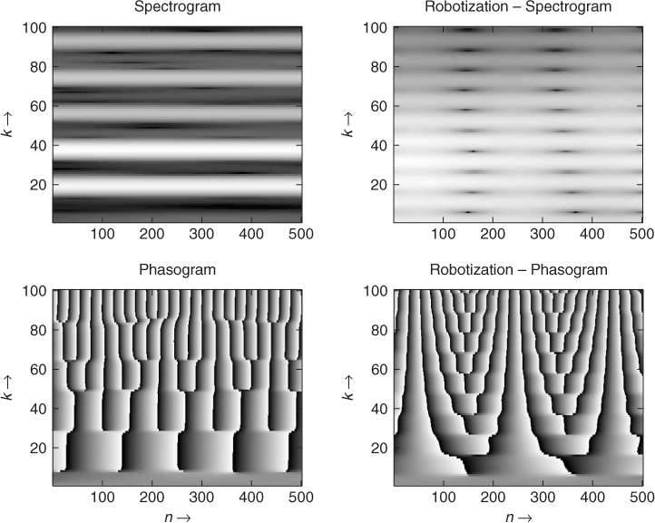
This is one of the shortest programs we can have, however its effect is very strong. The only drawback is that the n1 value in this program has to be an integer. The frequency of the robot is Fs/n1, where Fs is the sampling frequency. If the hop size is not an integer value, it is possible to use an interpolation scheme in order to dispatch the grain of two samples. This may happen if the hop size is calculated directly from a fundamental frequency value. An example is shown in Figure 7.30.
Figure 7.30 Example of robotization with a flute signal.
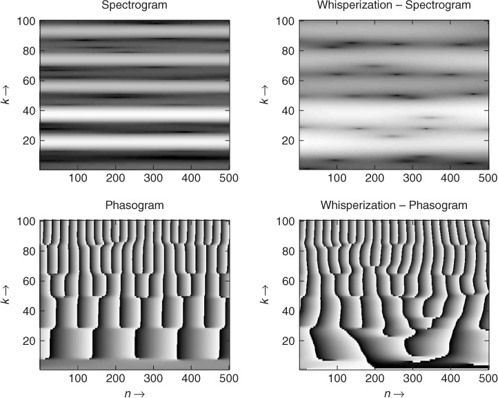
7.4.8 Whisperization
If we deliberately impose a random phase on a time-frequency representation, we can have a different behavior depending on the length of the window: if the window is quite large (for example, 2048 for a sampling rate of 44100 Hz), the magnitude will represent the behavior of the partials quite well and changes in phase will produce an uncertainty over the frequency. But if the window is small (e.g., 64 points), the spectral envelope will be enhanced and this will lead to a whispering effect. The M-file 7.17 implements the whisperization effect.
M-file 7.17 (VX_whisper.m)
% VX_whisper.m [DAFXbook, 2nd ed., chapter 7]
%===== This program makes the whisperization of a sound,
%===== by randomizing the phase
clear; clf
%----- user data -----
s_win = 512; % analysis window length [samples]
n1 = s_win/8; % analysis step [samples]
n2 = n1; % synthesis step [samples]
[DAFx_in,FS] = wavread(‘redwheel.wav’);
%----- initialize windows, arrays, etc -----
w1 = hanning(s_win, ‘periodic’); % analysis window
w2 = w1; % synthesis window
L = length(DAFx_in);
DAFx_in = [zeros(s_win, 1); DAFx_in; ...
zeros(s_win-mod(L,n1),1)] / max(abs(DAFx_in));
DAFx_out = zeros(length(DAFx_in),1);
tic
%UUUUUUUUUUUUUUUUUUUUUUUUUUUUUUUUUUUUUUU
pin = 0;
pout = 0;
pend = length(DAFx_in) - s_win;
while pin<pend
grain = DAFx_in(pin+1:pin+s_win).* w1;
%===========================================
f = fft(fftshift(grain));
r = abs(f);
phi = 2*pi*rand(s_win,1);
ft = (r.* exp(i*phi));
grain = fftshift(real(ifft(ft))).*w2;
% ===========================================
DAFx_out(pout+1:pout+s_win) = ...
DAFx_out(pout+1:pout+s_win) + grain;
pin = pin + n1;
pout = pout + n2;
end
%UUUUUUUUUUUUUUUUUUUUUUUUUUUUUUUUUUUUUUU
toc
%----- listening and saving the output -----
% DAFx_in = DAFx_in(s_win+1:s_win+L);
DAFx_out = DAFx_out(s_win+1:s_win+L) / max(abs(DAFx_out));
soundsc(DAFx_out, FS);
wavwrite(DAFx_out, FS, ‘whisper2.wav’);
It is also possible to make a random variation of the magnitude and keep the phase. An example is shown in Figure 7.31. This gives another way to implement whisperization, which can be achieved by the following MATLAB kernel:
%===========================================
f = fft(fftshift(grain));
r = abs(f).*randn(lfen,1);
phi = angle(f);
ft = (r.* exp(i*phi));
grain = fftshift(real(ifft(ft))).*w2;
%===========================================
Figure 7.31 Example of whisperization with a flute signal.
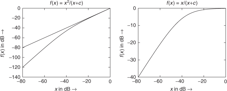
7.4.9 Denoising
A musician may want to emphasize some specific areas of a spectrum and lower the noise within a sound. Though this is achieved more perfectly by the use of a sinusoidal model (see Chapter 10), another approach is the use of denoising algorithms. The algorithm we describe uses a non-linear spectral subtraction technique [Vas96]. Further techniques can be found in [Cap94]. A time-frequency analysis and resynthesis are performed, with an extraction of the magnitude and phase information. The phase is kept as it is, while the magnitude is processed in such a way that it keeps the high-level values while attenuating the lower ones, in such a way as to attenuate the noise. This can also be seen as a bank of noise gates on different channels, because on each bin we perform a non-linear operation. The denoised magnitude vector Xd(n, k) = f(X(n, k)) of the denoised signal is then the output of a noise gate with a non-linear function f(x). A basic example of such a function is f(x) = x2/(x + c), which is shown in Figure 7.32. It can also be seen as the multiplication of the magnitude vector by a correction factor x/(x + c). The result of such a waveshaping function on the magnitude spectrum keeps the high values of the magnitude and lowers the small ones. Then the phase of the initial signal is reintroduced and the sound is reconstructed by overlapping grains with the help of an IFFT. The following M-file 7.18 follows this guideline.
M-file 7.18 (VX_denoise.m)
% VX_denoise.m [DAFXbook, 2nd ed., chapter 7]
%===== This program makes a denoising of a sound
clear; clf
%----- user data -----
n1 = 512; % analysis step [samples]
n2 = n1; % synthesis step [samples]
s_win = 2048; % analysis window length [samples]
[DAFx_in,FS] = wavread(‘redwheel.wav’);
%----- initialize windows, arrays, etc -----
w1 = hanning(s_win, ‘periodic’); % analysis window
w2 = w1; % synthesis window
L = length(DAFx_in);
DAFx_in = [zeros(s_win, 1); DAFx_in; ...
zeros(s_win-mod(L,n1),1)] / max(abs(DAFx_in));
DAFx_out = zeros(length(DAFx_in),1);
hs_win = s_win/2;
coef = 0.01;
freq = (0:1:299)/s_win*44100;
tic
%UUUUUUUUUUUUUUUUUUUUUUUUUUUUUUUUUUUUUUU
pin = 0;
pout = 0;
pend = length(DAFx_in) - s_win;
while pin<pend
grain = DAFx_in(pin+1:pin+s_win).* w1;
%===========================================
f = fft(grain);
r = abs(f)/hs_win;
ft = f.*r. / (r+coef);
grain = (real(ifft(ft))).*w2;
% ===========================================
DAFx_out(pout+1:pout+s_win) = ...
DAFx_out(pout+1:pout+s_win) + grain;
pin = pin + n1;
pout = pout + n2;
end
%UUUUUUUUUUUUUUUUUUUUUUUUUUUUUUUUUUUUUUU
toc
%----- listening and saving the output -----
% DAFx_in = DAFx_in(s_win+1:s_win+L);
DAFx_out = DAFx_out(s_win+1:s_win+L);
soundsc(DAFx_out, FS);
wavwrite(DAFx_out, FS, ‘x1_denoise.wav’);
Figure 7.32 Non-linear function for a noise gate.
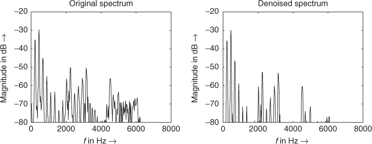
An example is shown in Figure 7.33. It is of course possible to introduce different noise-gate functions instead of the simple ones we have chosen. For instance, the formulation
ft = f.*r. / (r+coef);
can be replaced by the following one:
ft = f.*r. / max(r,coef);
With the first formulation, a bias is introduced to the magnitude of each frequency bin, whereas in the second formulaiton, the bias is only introduced for frequency bins that are actually denoised.
Figure 7.33 The left plot shows the windowed FFT of a flute sound. The right plot shows the same FFT after noise gating each bin using the r/(r+coef) gating function with c = 0.01.
Denoising in itself has many variations depending on the application:
1. Denoising from a tape recorder usually starts from the analysis of a noisy sound coming from a recording of silence. This gives a gaboret for the noise shape, so that the non-linear function will be different for each bin, and can be zero under this threshold.
2. The noise level can be estimated in a varying manner. For example, one can estimate a noise threshold which can be spectrum dependent. This usually involves spectral estimation techniques (with the help of LPC or cepstrum), which will be seen later.
3. One can also try to evaluate a level of noise on successive time instances in order to decrease pumping effects.
4. In any case, these algorithms involve non-linear operations and as such can produce artifacts. One of them is the existence of small grains that remain outside the silence unlike the previous noise (spurious components). The other artifact is that noise can sometimes be a useful component of a sound and will be suppressed as undesirable noise.
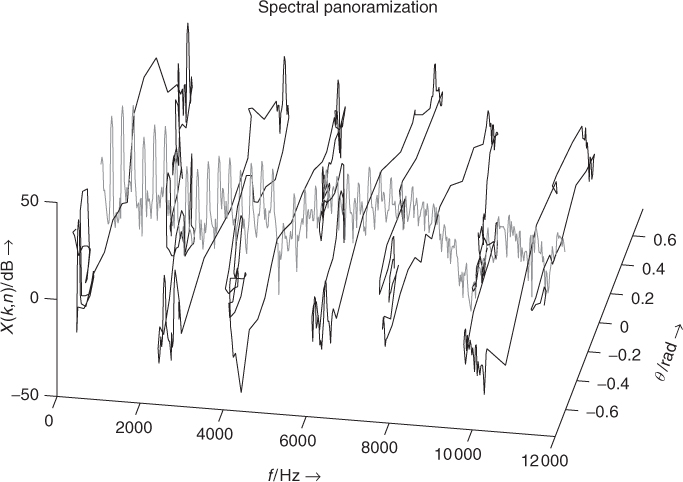
7.4.10 Spectral panning
Another sound transformation is to place sound sources in various physical places, which can be simulated in stereophonic sound by making use of azimuth panning. But what happens when trying to split the sound components? Then, each bin of the spectrum can be separately positioned using panning. Even better, by making use of the information from a phase-locked vocoder, one may put all frequency bins of the same component in the same angular position, avoiding the positioning artefacts that result from two adjacent bins that are coding for the same component and that would be otherwise placed in two different positions (the auditory image then being in the two places).
The Blumlein law [Bla83] for each sound sample is adapted to each frequency bin as
7.48 ![]()
where gL(n, k) and gL(n, k) are the time- and frequency-bin-varying gains to be applied to the left and right stereo channels, θ(n, k) is the angle of the virtual source position, and θl is the angle formed by each loudspeaker with the frontal direction. In the simple case where θl = 45° the output spectra are given by
7.49 ![]()
7.50 ![]()
A basic example is shown in Figure 7.34. Only the magnitude spectrum is modified: the phase of the initial signal is used unmodified, because this version of azimuth panning only modifies the gains, but not the fundamental frequency. This means that such effect does not simulate the Doppler effect. The stereophinc sound is then reconstructed by overlapping grains with the help of an IFFT. The following M-file 7.19 follows this guideline.
M-file 7.19 (VX_specpan.m)
% VX_specpan.m [DAFXbook, 2nd ed., chapter 7]
%===== This program makes a spectral panning of a sound
clear; clf
%----- user data -----
fig_plot = 1; % use any value except 0 or [] to plot figures
n1 = 512; % analysis step [samples]
n2 = n1; % synthesis step [samples]
s_win = 2048; % analysis window length [samples]
[DAFx_in,FS] = wavread(‘redwheel.wav’);
%----- initialize windows, arrays, etc -----
w1 = hanning(s_win, ‘periodic’); % analysis window
w2 = w1; % synthesis window
L = length(DAFx_in);
DAFx_in = [zeros(s_win, 1); DAFx_in; ...
zeros(s_win-mod(L,n1),1)] / max(abs(DAFx_in));
DAFx_out = zeros(length(DAFx_in),2);
hs_win = s_win/2;
coef = sqrt(2)/2;
%---- control: clipped sine wave with a few periods; in [-pi/4;pi/4]
theta = min(1,max(-1,2*sin((0:hs_win)/s_win*200))).' * pi/4;
% %---- control: rough left/right split at Fs/30 ˜ 1470 Hz
% theta = (((0:hs_win).'/2 < hs_win/30)) * pi/2 - pi/4;
%---- preserving phase symmetry ----
theta = [theta(1:hs_win+1); flipud(theta(1:hs_win-1))];
%---- drawing panning function ----
if (fig_plot)
figure;
plot((0:hs_win)/s_win*FS/1000, theta(1:hs_win+1));
axis tight; xlabel(‘f / kHz ightarrow’);
ylabel(‘ heta / rad ightarrow’);
title(‘Spectral panning angle as a function of frequency’)
end
tic
%UUUUUUUUUUUUUUUUUUUUUUUUUUUUUUUUUUUUUUU
pin = 0;
pout = 0;
pend = length(DAFx_in) - s_win;
while pin<pend
grain = DAFx_in(pin+1:pin+s_win).* w1;
%===========================================
f = fft(grain);
%---- compute left and right spectrum with Blumlein law at 45°
ftL = coef * f .* (cos(theta) + sin(theta));
ftR = coef * f .* (cos(theta) - sin(theta));
grainL = (real(ifft(ftL))).*w2;
grainR = (real(ifft(ftR))).*w2;
% ===========================================
DAFx_out(pout+1:pout+s_win,1) = ...
DAFx_out(pout+1:pout+s_win,1) + grainL;
DAFx_out(pout+1:pout+s_win,2) = ...
DAFx_out(pout+1:pout+s_win,2) + grainR;
pin = pin + n1;
pout = pout + n2;
end
%UUUUUUUUUUUUUUUUUUUUUUUUUUUUUUUUUUUUUUU
toc
%----- listening and saving the output -----
% DAFx_in = DAFx_in(s_win+1:s_win+L);
DAFx_out = DAFx_out(s_win+1:s_win+L,:) / max(max(abs(DAFx_out)));
soundsc(DAFx_out, FS);
wavwrite(DAFx_out, FS, ‘x1_specpan.wav’);
Figure 7.34 Spectral panning of the magnitude spectrum of a single frame, using a wave form as the panning angle. Each frequency bin of the original STFT X(n, k) (centered with θ = 0, in gray) is panoramized with constant power.
Spectral panning offers many applications, which are listed to show the variety of possibilities:
1. Pseudo-source separation when combined with a multi-pitch detector.
2. Arbitrary panning when the θ(n, k) value is not related to the spectral content of the sound.
3. Vomito effect, when the azimuth angles are refreshed too often (i.e., every frame at a 50 Hz rate), the fast motions of sound also implies timbre modulations (as the amplitude modulation has a frequency higher than 20 Hz), both of which result in some unpleasant effects for the listener.