12.3 Circuit-based Valve Emulation

Digital emulation of valve- or vacuum-tube amplifiers is currently a vibrant area of research with many commercial applications. As explained in a recent review article [PY09], most existing digital valve-emulation methods may roughly be divided into static waveshapers, custom nonlinear filters, and circuit-simulation-based techniques. The first type of these methods, static waveshapers (e.g., [Sul90, Kra91, AS96, Shi96, DMRS98, FC01, MGZ02, Jac03, Ame03, SST07, SM07]), use memoryless nonlinear functions for creating signal distortion and linear filtering before and after the nonlinearity for tuning the magnitude response. Oversampling is usually used to avoid signal aliasing.

12.3.1 Dynamic Nonlinearities and Impedance Coupling

Although the valve component itself is mainly a memoryless device that can in principle be approximated with static nonlinear functions, reactive components (typically capacitors) in the circuit make the nonlinearity act as dynamic. This means that in reality, the shape of the nonlinearity changes according to the input signal and the internal state of the circuit. Custom nonlinear valve emulation filters [Pri91, KI98, GCO+04, KMKH06] simulate this dynamic nonlinearity, for example by creating a feedback loop around the nonlinearity.

Another important phenomenon in real valve circuits is the two-directional impedance coupling between components and different parts of the circuit. This causes, for example, an additional signal-dependent bias variation of a valve circuit when connected to a reactive load, such as a loudspeaker. If the digital valve circuit model uses a unidirectional signal path—as many simple models do—altering some part in the virtual circuit has no effect on the parts earlier in the signal chain. For example, if a linear loudspeaker model is attached to a virtual tube circuit with unidirectional signal flow, the resulting effect will only be a linear filtering according to the transfer characteristics of the loudspeaker, and no coupling effects with the tube circuit will be present. Nonlinear circuit-simulation-based modeling techniques (e.g., [Huo04, Huo05, YS08, YAAS08, Gal08, MS09]) try to incorporate the impedance coupling effect, at least between some parts of the circuit. Traditionally, these methods use Kirchhoff's rules and energy conservation laws to manually obtain the ordinary differential equations (ODEs) that represent the operation of the circuit. The ODEs are then discretized (usually using the bilinear transform), and the system of implicit nonlinear equations is iteratively solved using numerical integration methods, such as the Newton—Raphson or Runge—Kutta.

12.3.2 Modularity

From the digital valve-amplifier designer's point of view, modularity would be a desirable property for the emulator. In an ideal system, it should be easy to edit the circuit topology, for example by graphically altering the circuit schematics, and the sonic results should be immediately available. Enabling full control over the digital circuit construction would allow the emulation of any vintage valve amplifier simply by copying its circuit schematics into the system. Furthermore, it would enable the designer to apply the knowledge of valve-amplifier building tradition into the novel digital models. Note that this would mean that the designer should not be limited by conventional circuit design constraints or even general physical laws in creating a new digital amplifier, so that also purely digital or “abstract” processing techniques could well be used in conjunction. In the late 1990s, several valve circuit models (for example [Ryd95, Lea95, PLBC97, Sju97]) were presented for the SPICE circuit simulator software [QPN+07]. Although these models were modular and able to simulate the full impedance coupling within the whole system, they could not be used as real-time effects due to their intensive computational load. In fact, even over a decade later, these SPICE models are computationally still too heavy to run in real time.

Wave digital filters (WDFs), introduced by Fettweis [Fet86], offer a modular and relatively light approach for real-time circuit simulation. The main difference between WDFs and most other modeling methods is that WDFs represent all signals and states as wave variables and use local discretization for the circuit components. The WDF method will be explained more thoroughly in Section 12.3.3, and a simple nonlinear circuit simulation example using WDFs is presented in Section 12.3.4. The K-method, a state-space approach for the simulation of nonlinear systems has been introduced by Borin and others [BPR00]. This alternative approach for circuit simulation is currently another promising candidate for real-time valve simulation. It should be noted that although state-space models are not inherently modular, a novel technique by Yeh [Yeh09] allows the automatization of the model-building process, so that state-space simulation models may automatically be obtained from a circuit schematics description.

12.3.3 Wave Digital Filter Basics

The basics of WDF modeling are briefly reviewed in the following section. A signal-processing approach has been chosen with less emphasis on the physical modeling aspects, in order to clarify the operation of the modeling example in Section 12.3.4. For a more thorough tutorial on WDFs, see, for example [Fet86, VPEK06].

One-port Elements

WDF components connect to each other using ports. Each port has two terminals, one for transporting incoming waves, and one for transporting outgoing waves. Also, each port has an additional parameter, port resistance, which is used in implementing proper impedance coupling between components. The relationship between the Kirchhoff pair (e.g., voltage U and current I) and wave variables A and B is given by

12.14

where denotes the port resistance.

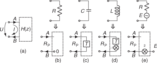
Note that this port resistance is purely a computational parameter, and it should not be confused with electrical resistance. Most elementary circuit components can be represented using WDF one-port elements. Some basic circuit components are illustrated together with their WDF one-port counterparts in Figure 12.11. Some other circuit components, such as transformers, cannot be represented as one-port elements, but require a multiport representation, which is out of the scope of this book. The port resistances of the one-port elements in Figure 12.11 can be given as follows:

12.15

where R, C and L are the electrical resistance (Ohms), capacitance (Farads), and inductance (Henrys), respectively, while stands for the sample rate (Hertz). Similar to the WDF resistor, the port resistance of a voltage source is equivalent to the physical resistance.

Figure 12.11 Basic WDF one-port elements: (a) a generic one-port with voltage U across and current I across the terminals, (b) resistor, (c) capacitor, (d) inductor, (e) voltage source. Here, A represents an incoming wave for each element, while B denotes an outgoing wave. Symbol stands for the port resistance. Figure adapted from [PK10] and reprinted with IEEE permission

Adaptors

The WDF circuit components connect to each other via adaptors. In practice, the adaptors direct signal routing inside the WDF circuit model, and implement the correct impedance coupling via port resistances. Although the number of ports in an adaptor is not limited in principle, three-port adaptors are typically used, since any N-port adaptor (N > 3) can be expressed using a connection of three-port adaptors, so that the whole WDF circuit becomes a binary tree structure [DST03]. There are two types of WDF adaptors: series and parallel, which implement the series and parallel connection between elements, respectively. Furthermore, the port resistance values for the adaptors should be set equal to the port resistances of the elements they are connected to.

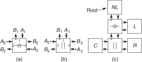
Figures 12.12(a) and (b) illustrate the WDF series and parallel adaptors, respectively. Here, the ports have been numbered, for clarity. The outgoing wave Bn at port n = 1, 2, 3 of a three-port adaptor can generally be expressed as

12.16

where An denotes the incoming wave at port n and Gn = 1/Rn is the inverse of the port resistance Rn.

Figure 12.12 WDF three-port serial (a) and parallel (b) adaptors and an example WDF binary tree (c).

Computational Scheduling

Figure 12.12(c) depicts an example WDF binary tree, simulating an RLC circuit with a nonlinear resistor (marked NL in the figure). As can be seen, the adaptors act as nodal points connecting the one-port elements together. For this reason, the adaptors in a WDF binary tree are also called nodes, and the one-port elements are called the leaves of the binary tree. When deciding the order of computations, a single one-port element must be chosen as the root of the tree. In Figure 12.12(c), the nonlinear resistor is chosen as the root. When this decision has been made, the WDF simulation starts by first evaluating all the waves propagating from the leaves towards the root. When the incoming wave arrives at the root element, the outgoing wave is computed, and the waves are propagated from the root towards the leaves, after which the process is repeated.

As can be seen in Equation (12.16), the wave leaving the WDF adaptor is given as a function of the incoming waves and port resistances. This poses a problem for the computation schedule discussed above, since in order for the adaptor to compute the waves towards the root, it would also have to know the wave coming from the root at the same time. Interestingly, the port resistances can be used as a remedy. By properly selecting the port resistance for the port facing the root, the wave traveling towards the root can be made independent from the wave traveling away from the root.

For example, if we name the port facing the root element as port number one, and set its port resistance as R1 = R2 + R3 if it is a series adaptor (and the inverse port resistance G1 = G2 + G3 if it is a parallel adaptor), Equation (12.16) simplifies into

12.17

for the wave components traveling towards the root. In our example, the port number one would be called adapted, or reflection free, since the outgoing wave does not depend on the incoming (reflected) wave. Such adapted ports are typically denoted with a “T-shaped” ending for the outwards terminal, as illustrated for port number one in Figure 12.12(a) and (b). As Figure 12.12(c) shows, all adapted ports point towards the root.

Since the root element is connected to an adapted port, and the port resistances between the adapted port and the root should be equal, an interesting paradox arises. On one hand, the shared port resistance value should be set as required by the adaptor (for example as the sum of the other port resistances on a series adaptor), but on the other hand, the port resistance should be set as dictated by the root element (for example as a resistance value in Ohms for a resistor). If a resistor is chosen as a root element, the solution is to define the outgoing wave B from the root as [Kar]

12.18

where R is the electrical resistance of the root, is the port resistance set by the adapted port, and A is the wave going into the root element. Since the port resistance of the adapted port is independent of the electrical resistance of the root, the latter can freely be varied during simulation without encountering computability problems. Thus, if the circuit has a nonlinear one-port element, it should be chosen as the root for the WDF tree (since nonlinearity can be seen as parametric variation at a signal rate). For all other leaves, changing the port resistance during simulation is problematic since correct operation would require the port resistance changes to be propagated throughout the whole tree and iterated to correctly set the changed wave values. In practice, however, it is possible to vary the port resistances (i.e., component values) of the leaves without problems, provided that the parametric variation is slow compared to the sampling rate of the system.

Nonlinearities and Model Initialization

In a nonlinear resistor, the electrical resistance value depends nonlinearly on the voltage over the resistor, and a correct simulation of this implicit nonlinearity requires iterative techniques in general. Note the difference between the earlier discussed global iteration for setting the values of all port resistances, and the local iteration to set only the value of the nonlinear resistor: although the adapted ports remove the need for the former, one should still in principle perform the latter. Since run-time iteration is a computationally intensive operation, a typical practical simplification for avoiding local iteration is to insert an additional unit delay to the system, for example by using the voltage value at the previous time instant when calculating the resistance value. The error caused by this extra delay is usually negligible, provided that the shape of the nonlinearity is relatively smooth, as is the case with typical valve components. Further information on nonlinear WDFs can be found in [SD99, Bil01]. Valve simulation using WDFs was first presented in [KP06], and refined models have been discussed in [PTK09, PK10].

Reactive WDF circuit components should be correctly initialized before the simulation starts. This means that the one-sample memory of inductors and capacitors should be set so that the voltages and currents comply with Kirchhoff's laws. For reactive components that have nonzero initial energy (for example an initially charged capacitor), this can be tricky since the relationship between the stored energy and the wave value inside the memory is not straightforward. However, the correct initialization procedure can still be performed by using Thévenin or Norton equivalents. A practical alternative is to set the memory of reactive WDF components to zero, and let the simulation run for some “warm-up” time before inserting the actual input signal so that a steady operating point is reached and the reactances have been properly charged. In a sense, this is similar to letting a real electric circuit warm up and reach the correct operating point before feeding the input signal.

Remaining Challenges in WDF Modeling

Although WDFs have many desirable properties in circuit-simulation applications, there are also some open research problems related to them that limit their usability on a large scale. Probably the most severe limitation is that those circuit topologies that do not map onto binary trees are difficult to realize. Such topologies include bridge connections and loop-like structures. Modeling of bridge connections using WDFs is further discussed in [Kar08]. Another limitation is that a WDF binary tree can generally have only a single nonlinear element. If multiple nonlinearities are to be simulated using WDFs, global iteration should be applied for the whole sub-tree connecting the nonlinearities to each other. Alternatively, unit delays can be inserted into the system to enable computability, as done in [PK10], but this may drastically affect the stability of the system in some cases.

12.3.4 Diode Circuit Model Using Wave Digital Filters

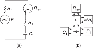
This section discusses a WDF representation of a simple valve diode circuit, depicted in Figure 12.13(a). The WDF equivalent of the electric circuit is illustrated in Figure 12.13(b). The simulator algorithm is implemented using object-oriented programming for illustrating the inherent modularity of WDFs. The related code requires a basic understanding of object-oriented programming principles, and is mainly intended to show the possibilities of WDF modeling, rather than trying to provide a computationally efficient implementation. The class files are defined in the M-file 12.6, and the diode circuit model is presented in M-file 12.7. The presented WDF simulator consists of seven classes, three of which are abstract (i.e., they only serve as superclasses to real classes). It must be noted that all the presented classes are shown in a single M-file for compactness although in practice MATLAB requires each class to reside in an individual file. In other words, the classes in M-file 12.6 should be split into seven different files in order for the model to run in MATLAB.

Figure 12.13 Electrical (a) and WDF (b) representations of an RC circuit with a vacuum-tube diode. The diode is denoted , since it is realized as a nonlinear resistor as the root element of the binary WDF tree structure.

The first class in M-file 12.6 defines the WDF superclass, which serves as a parent for the other six classes. The WDF class itself is inherited from MATLAB's hgsetget-class, which results in all WDF elements being handle-objects. This means that when object properties (such as wave variable values) are edited, MATLAB only modifies the property values, instead of creating entirely new objects. The PortRes property defines the port resistance of a WDF object, and the Voltage method gives the voltage over the element, as defined in Equation (12.14). The next class in M-file 12.6 defines the Adaptor class, which serves as a superclass for three-port series and parallel adaptors. Two properties, KidLeft and KidRight, are defined, which serve as handles to the WDF objects connected to the adaptor.

The ser class defines the WDF series adaptor. The waves traveling up (towards the root) and down (away from the root) are given as properties WU and WD, respectively. The adaptor is realized so that the adapted port always points up, to enable the connection of a nonlinear element at the root. In addition to the class constructor, this class defines two methods, WaveUp and set.WD. The first of these reads the up-going wave according to Equation (12.17), and the second sets the down-going waves for the connected elements according to Equation (12.16). Note that the parallel adaptor is similarly defined and can be found among the supplementary MATLAB-files on-line, although it is omitted here for brevity.

The OnePort class in M-file 12.6 serves as a superclass for all one-port WDF elements. It also defines the up- and down-going waves WU and WD and the set.WD-method. This method also updates the internal state, or memory, of a reactive WDF one-port. The last three classes in M-file 12.6 introduce the classes R, C, and V, which represent the WDF resistors, capacitors, and voltage sources, respectively. Note that the class L for implementing a WDF inductor may easily be edited from the C class, although it is not printed here (but included in the associated on-line code).

The actual diode simulation example is printed as M-file 12.7, and will be briefly explained here. M-file 12.7 starts by defining the overall simulation parameters and variables, such as the sample rate, and input and output signals. Next, the WDF elements (resistive voltage source, resistor, and a capacitor) are created, and the WDF is formed as a series connection. The nonlinear resistor is not created as an object, but it is manually implemented in the simulation loop.

The simulation loop starts by reading the input signal as the source voltage for object V1. Next, the WaveUp method is called for the WDF tree, resulting in all up-going waves to be propagated at the root. The valve resistor is modeled as the nonlinear resistance

12.19

as a function of the voltage U over the diode. Equation (12.19) was empirically found to be a simple, but fairly accurate simulation of a GZ 34 valve diode. Here, the previous value of the diode voltage is used, in order to avoid the local iteration of the implicit nonlinearity. The wave reflection at the nonlinearity is implemented according to Equation (12.18), and the down-going waves are propagated to the leaves. Finally, the diode voltage is updated for the next time sample, and the output is read as the voltage over the resistor R1. After the simulation loop is finished, the results are illustrated using the plot-commands.

It is important to note, that due to the modularity of the WDFs and the object-oriented nature of the implementation, editing of the simulation circuit is very easy. All that has to be done to simulate a different circuit is to change the one-port element definitions (rows 10-13 in M-file 12.7) and the circuit topology (row 14 in M-file 12.7). In other words, M-files 12.6 and 12.7 define an entire circuit simulation software!

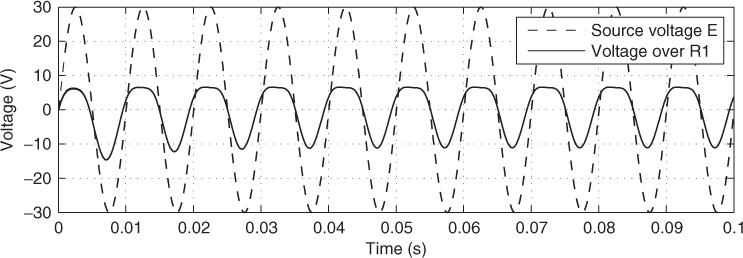
The output of the WDF model, i.e., the circuit response to a 100 Hz sine signal is illustrated in Figure 12.14. As expected, the positive signal peaks have been squashed since the diode lets forward current pass, reducing the potential difference over the diode. This current also charges the capacitor, reducing the voltage drop for negative signal cycles in the beginning of the simulation. Thus, Figure 12.14 visualizes both the static nonlinearity due to the diode component itself, as well as the dynamic behavior caused by the capacitance. The simulation results were verified using LTSpice simulation for the same circuit. The resulting waveforms were visually identical for both the WDF and LTSpice simulations.

Figure 12.14 Voltage over the tube diode, as plotted by the M-file 12.7. As can be seen, the diode nonlinearity has squashed the positive signal peaks, while charging of the capacitor causes a shift in the local minima.