12
Dynamic programming

In this chapter we begin our discussion of multistage decision problems, where multiple decisions have to be made over time and with varying degrees of information. The salient aspect of multistage decision making is that, like in a chess game, decisions made now affect the worthiness of options available in the future and sometimes also the information available when making future decisions. In statistical practice, multistage problems can be used to provide a decision-theoretic foundation to the design of experiments, in which early decisions are concerned with which data to collect, and later decisions with how to use the information obtained. Chapters 13, 14, and 15 consider multistage statistical decisions in some detail. In this chapter we will be concerned with the general principles underlying multistage decisions for expected utility maximizers.

Finite multistage problems can be represented by decision trees. A decision tree is a graphical representation that allows us to visualize a large and complex decision problem by breaking it into smaller and simpler decision problems. In this chapter, we illustrate the use of decision trees in the travel insurance example of Section 7.3 and then present a general solution approach to two-stage (Section 12.3.1) and multistage (Section 12.3.2) decision trees. Examples are provided in Sections 12.4.1 through 12.5.2. While conceptually general and powerful, the techniques we will present are not of easy implementation: we will discuss some of the computational issues in Section 12.7.

The main principle used in solving multistage decision trees is called backwards induction and it emerged in the 1950s primarily through the work of Bellman (1957) on dynamic programming.

Featured book (chapter 3):

Bellman, R. E. (1957). Dynamic programming, Princeton University Press.

Our discussion is based on Raiffa and Schlaifer (1961). Additional useful references are DeGroot (1970), Lindley (1985), French (1988), Bather (2000), and Bernardo and Smith (2000).

12.1 History

Industrial process control has been one of the initial motivating applications for dynamic programming algorithms. Nemhauser illustrates the idea as follows:

The technique just described to solve multidimensional decision problems is called dynamic programming, and is based on the principle of backwards induction. Backwards induction has its roots in the work of Arrow et al. (1949) on optimal stopping problems and that of Wald (1950) on sequential decision theory. In optimal stopping problems one has the option to collect data sequentially. At each decision node two options are available: either continue sampling, or stop sampling and take a terminal action. We will discuss this class of problems in some detail in Chapter 15. Richard Bellman’s research on a large class of sequential problems in the early 1950s led to the first book on the subject (Bellman 1957) (see also Bellman and Dreyfus 1962). Bellman also coined the term dynamic programming:

A far more colorful description of the political motivation behind this choice is reported in Bellman’s autobiography (Bellman 1984), as well as in Dreyfus (2002).

The expression backward induction comes from the fact that the sequence of decisions is solved by reversing their order in time, as illustrated with the chemical example by Nemhauser (1966). Lindley explains the inductive technique as follows:

The dynamic programming method allows us to conceptualize and solve problems that would be far less tractable if each possible decision function, which depends on data and decisions that accumulate sequentially, had to be considered explicitly:

Roughly speaking, the technique allows one to transform a multistage decision problem into a series of one-stage decision problems and thus make decisions one at a time. This relies on the principle of optimality stated by Bellman:

This ultimately allows for computational advantages as explained by Nemhauser:

Dynamic programming algorithms have found applications in engineering, economics, medicine, and most recently computational biology, where they are used to optimally align similar biological sequences (Ewens and Grant 2001).

12.2 The travel insurance example revisited

We begin our discussion of dynamic programming techniques by revisiting the travel insurance example of Section 7.3. In that section we considered how to optimally use the information about the medical test. We are now going to consider the sequential decision problem in which, in the first stage, you have to decide whether or not to take the test, and in the second stage you have to decide whether or not to buy insurance. This is an example of a two-stage sequential decision problem. Two-stage or, more generally, multistage decision problems can be represented by decision trees by introducing additional decision nodes and chance nodes. Figure 12.1 shows the decision tree for this sequential problem.

In this example we use the loss function in the original formulation given in Table 7.6. However, as previously discussed, the Bayesian solution would be the same should we use regret losses instead, and this still applies in the multistage case.

We are going to work within the expected utility principle, and also adhere to the before/after axiom across all stages of decisions. So we condition on information as it accrues, and we revise our probability distribution on the states of the world using the Bayes rule at each stage. In this example, to calculate the Bayes strategy we need to obtain the posterior probabilities of becoming ill given each of the possible values of x, that is

Figure 12.1 Decision tree for the two-stage travel insurance example.

for θ = θ₁, θ₂ and x = 0, 1. Here

is the marginal distribution of x. We get

m(x = 1) =	0.250
π(θ1|x = 0) =	0.004
π(θ1|x = 1) =	0.108.

Hence, we can calculate the posterior expected losses for rules δ₁ and δ₂ given x = 0 as

δ1 :	Expected loss = 1000 × 0.004 + 0 × 0.996 = 4
δ2 :	Expected loss = 50 × 0.004 + 50 × 0.996 = 50

and given x = 1 as

δ1 :	Expected loss = 50 × 0.108 + 50 × 0.892 = 50
δ2 :	Expected loss = 1000 × 0.108 + 0 × 0.892 = 108.

The expected losses for rules δ₀ and δ₃ remain as they were, because those rules do not depend on the data. Thus, if the test is performed and it turns out positive, then the optimal decision is to buy the insurance and the expected loss of this action is 50. If the test is negative, then the optimal decision is not to buy the insurance with expected loss 4. Incidentally, we knew this from Section 7.3, because we had calculated the Bayes rule by minimizing the Bayes risk. Here we verified that we get the same result by minimizing the posterior expected loss for each point in the sample space.

Now we can turn to the problem of whether or not to get tested. When no test is performed, the optimal solution is not to buy the insurance, and that has an expected loss of 30. When a test is performed, we calculate the expected losses associated with the decision in the first stage from this perspective: we can evaluate what happens if the test is positive and we proceed according to the optimal strategy thereafter. Similarly, we can evaluate what happens if the test is negative and we proceed according to the optimal strategy thereafter. So what we expect to happen is a weighted average of the two optimal expected losses, each conditional on one of the possible outcomes of x. The weights are the probabilities of the outcomes of x at the present time. Accordingly, the expected loss if the test is chosen is

50 × m(x = 1) + 4 × m(x = 0) = 50 × 0.25 + 4 × 0.75 = 15.5.

Comparing this to 30, the value we get if we do not test, we conclude that the optimal decision is to test. This is reassuring: the test is free (so far) and the information provided by the test would contribute to our decision, so it is logical that the optimum at the first stage is to acquire the information. Overall, the optimal sequential strategy is as follows. You should take the test. If the test is positive, then buy the medical insurance. If the test is negative, then you should not buy the medical insurance. The complete analysis of this decision problem is summarized in Figure 12.2.

Lindley comments on the rationale behind solving a decision tree:

In our calculations so far we ignored the costs of testing. How would the solution change if the cost of testing was, say, $10? All terminal branches that stem out from the action “test” in Figure 12.2 would have the added cost of $10. This would imply that the expected loss for the action “test” would be 25.5 while the expected loss for the action “no test” would still be 30.0. Thus, the optimal decision would still be to take the test. The difference between the expected loss of 30 if no test information is available and that of 15.5 if the test is available is the largest price you should be willing to pay for the test. In the context of this specific decision this difference measures the worthiness of the information provided by the test—a theme that will return in Chapter 13.

Figure 12.2 Solved decision tree for the two-stage travel insurance example. Losses are given at the end of the branches. Above each chance node is the expected loss, while above each decision node is the maximum expected utility. Alongside the branches stemming from each chance node are the probabilities of the states of nature. Actions that are not optimal are crossed out by a double line.

Here we worked out the optimal sequential strategy in stages, by solving the insurance problem first, and then nesting the solution into the diagnostic test problem. Alternatively, we could have laid out all the possible sequential strategies. In this case there are six:

Stage 1	Stage 2
Do not test	Do not buy the insurance
Do not test	Buy the insurance
Test	Do not buy the insurance
Test	Buy the insurance if x = 1. Otherwise, do not
Test	Buy the insurance if x = 0. Otherwise, do not
Test	Buy the insurance

We could alternatively figure out the expected loss of each of these six options, and pick the one with the lowest value. It turns out that the answer would be the same. This is an instance of the equivalence between the normal form of the analysis—which lists all possible decision rules as we just did—and the extensive form of analysis, represented by the tree. We elaborate on this equivalence in the next section.

12.3 Dynamic programming

12.3.1 Two-stage finite decision problems

A general two-stage finite decision problem can be represented by the decision tree of Figure 12.3. As in the travel insurance example, the tree represents the sequential problem with decision nodes shown in a chronological order.

To formalize the solution we first introduce some additional notation. Actions will carry a superscript in brackets indicating the stage at which they are available. So are the actions available at stage s. In Figure 12.3, s is either 1 or 2. For each action at stage 1 we have a set of possible observations that will potentially guide the decision at stage 2. For action these are indicated by x_i1, ..., x_iJ. For each action at stage 2 we have the same set of possible states of the world θ₁, ..., θ_K, and for each combination of actions and states of the world, as usual, an outcome z. If actions and are chosen and θ_k is the true state of the world, the outcome is z_i1i2k. A warning about notation: for the remainder of the book, we are going to abandon the loss notation in favor of the utility notation used in the discussion of foundation. Finally, in the above, we assume an equal number of possible states of the world and outcomes to simplify notation. A more general formulation is given in Section 12.3.2.

In our travel insurance example we used backwards induction in that we worked from the outermost branches of the decision tree (the right side of Figure 12.3) back to the root node on the left. We proceeded from the terminal branches to the root by alternating the calculation of expected utilities at the random nodes and maximization of expected utilities at the decision nodes. This can be formalized for a general two-stage decision tree as follows.

Figure 12.3 A general two-stage decision tree with finite states of nature and data.

At the second stage, given that we chose action in the first stage, and that outcome x_i1j was observed, we choose a terminal action a^*(2) to achieve

At stage 2 there only remains uncertainty about the state of nature θ. As usual, this is addressed by taking the expected value of the utilities with respect to the posterior distribution. We then choose the action that maximizes the expected utility. Expression (12.1) depends on i₁ and j, so this maximization defines a function which provides us with a recipe for how to optimally proceed in every possible scenario. An important difference with Chapter 7 is the dependence on the first-stage decision, typically necessary because different actions may be available for δ⁽²⁾ to choose from, depending on what was chosen earlier.

Equipped with δ^*(2), we then step back to stage 1 and choose an action a^*(1) to achieve

The inner maximum is expression (12.1) and we have it from the previous step. The outer summation in (12.2) computes the expected utility associated with choosing the i₁th action at stage 1, and then proceeding optimally in stage 2. When the stage 1 decision is made, the maximum expected utilities ensuing from the available actions are uncertain because the outcome of x is not known. We address this by taking the expected value of the maximum utilities calculated in (12.1) with respect to the marginal distribution of x, for each action . The result is the outer summation in (12.2). The optimal solution at the first stage is then the action that maximizes the outer summation. At the end of the whole process, an optimal sequential decision rule is available in the form of a pair (a^*(1), δ^*(2)).

To map this procedure back to our discussion of optimal decision functions in Chapter 7, imagine we are minimizing the negative of the function u in expression (12.2). The innermost maximization is the familiar minimization of posterior expected loss. The optimal a^*(2) depends on x. In the terminology of Chapter 7 this optimization will define a formal Bayes rule with respect to the loss function given by the negative of the utility. The summation with respect to j computes an average of the posterior expected losses with respect to the marginal distribution of the observations, and so it effectively is a Bayes risk r, so long as the loss is bounded. In the two-stage setting we get a Bayes risk for every stage 1 action , and then choose the action with the lowest Bayes risk. We now have a plan for what to do at stage 1, and for what to do at stage 2 in response to any of the potential experimental outcomes that result from the stage 1 decision.

In this multistage decision, the likelihood principle operates at stage 2 but not at stage 1. At stage 2 the data are known and the alternative results that never occurred have become irrelevant. At stage 1 the data are unknown, and the distribution of possible experimental results is essential for making the experimental design decision.

Another important connection between this discussion and that of Chapter 7 concerns the equivalence of normal and extensive forms of analysis. Using the Bayes rule we can rewrite the outer summation in expression (12.2) as

The function δ* that is defined by maximizing the inner sum pointwise for each i and j will also maximize the average expected utility, so we can rewrite the right hand side as

Here δ is not explicitly represented in the expression in square brackets. Each choice of δ specifies how subscript i₂ is determined as a function of i₁ and j. Reversing the order of summations we get

Lastly, inserting this into expression (12.2) we obtain an equivalent representation as

This equation gives the solution in normal form: rather than alternating expectations and maximizations, the two stages are maximized jointly with respect to pairs (a⁽¹⁾, δ⁽²⁾). The inner summation gives the expected utility of a decision rule, given the state of nature, over repeated experiments. The outer summation gives the expected utility of a decision rule averaging over the states of nature. A similar equivalence was brought up earlier on in Chapter 7 when we discussed the relationship between the posterior expected loss (in the extensive form) and the Bayes risk (in the normal form of analysis).

12.3.2 More than two stages

We are now going to extend these concepts to more general multistage problems, and consider the decision tree of Figure 12.4. As before, stages are chronological from left to right, information may become available between stages, and each decision is dependent on decisions made in earlier stages. We will assume that the decision tree is bounded, in the sense that there is a finite number of both stages and decisions at each stage.

First we need to set the notation. As before, S is the number of decision stages. Now are the decisions available at the sth stage, with s = 1, ..., S. At each stage, the action is different from the rest in that, if is taken, no further stages take place, and the decision problem terminates. Formally maps states to outcomes in the standard way. For each stopping action we have a set of relevant states of the world that constitute the domain of the action. At stage s, the possible states are . For each continuation action , we observe a random variable with possible values . If stage s is reached, the decision may depend on all the decisions that were made, and all the information that was accrued in preceding stages. We concisely refer to this information as the history, and use the notation H_s−1 where

For completeness of notation, the (empty) history prior to stage 1 is denoted by H₀. Finally, at the last stage S, the set of states of the world constituting the domain of action is .

Figure 12.4 Decision tree for a generic multistage decision problem.

It is straightforward to extend this setting to the case in which J_s also depends on i without any conceptual modification. We avoid it here for notational simplicity.

Dynamic programming proceeds as follows. We start by solving the decision problem from the last stage, stage S, by maximizing expected utility for every possible history. Then, conditional on the optimal choice made at stage S, we solve the problem at stage S – 1, by maximizing again the expected maximum utility. This procedure is repeated until we solve the decision problem at the first stage. Algorithmically, we can describe this recursive procedure as follows:

1. At stage S:

   1. For every possible history H_S−1, compute the expected utility of the actions , i = 0,..., I_s, available at stage S, using

      

      where .

   2. Obtain the optimal action, that is

      

      This is a function of H_S−1 because both the posterior distribution of θ and the utility of the outcomes depend on the past history of decisions and observations.

2. For stages S – 1 through 1, repeat:

   1. For every possible history H_s−1, compute the expected utility of actions , i = 0,..., I_s, available at stage s, using

      

      where now are the expected utilities associated with the optimal continuation from stage s + 1 on, given that that is chosen and occurs. If we indicate by the resulting history, then we have

      

      A special case is the utility of the decision to stop, which is

      

   2. Obtain the optimal action, that is

      

   3. Move to stage s – 1, or stop if s = 1.

This algorithm identifies a sequence of functions a^*(s)(H_s−1), s = 1, ..., S, that defines the optimal sequential solution.

In a large class of problems we only need to allow z to depend on the unknown θ and the terminal action. This still covers problems in which the first S – 1 stages are information gathering and free, while the last stage is a statistical decision involving θ. See also Problem 12.4. We now illustrate this general algorithm in two artificial examples, and then move to applications.

12.4 Trading off immediate gains and information

12.4.1 The secretary problem

For an application of the dynamic programming technique we will consider a version of a famous problem usually referred to in the literature under a variety of politically incorrect denominations such as the “secretary problem” or the “beauty-contest problem.” Lindley (1961), DeGroot (1970), and Bernardo and Smith (1994) all discuss this example, and there is a large literature including versions that can get quite complicated. The reason for all this interest is that this example, while relatively simple, captures one of the most fascinating sides of sequential analysis: that is, the ability of optimal solutions to negotiate trade-offs between immediate gains and information-gathering activities that may lead to greater future gains.

We decided to make up yet another story for this example. After successful interviews in S different companies you are the top candidate in each one of them. One by one, and sequentially, you are going to receive an offer from each company. Once you receive an offer, you may accept it or you may decline it and wait for the next offer. You cannot consider more than one offer at the time, and if you decide to decline an offer, you cannot go back and accept it later. You have no information about whether the offers that you have not seen are better or worse than the ones you have seen: the offers come in random order. The information you do have about each offer is its relative rank among the offers you previously received. This is reasonable if the companies are more or less equally desirable to you, but the conditions of the offers vary. If you refuse all previous offers, and you reach the Sth stage, you take the last offer.

When should you accept an offer? How early should you do it and how high should the rank be? If you accept too soon, then it is possible that you will miss the opportunity to take better future offers. On the other hand, if you wait too long, you may decline offers that turn out to be better than the one you ultimately accept. Waiting gives you more information, but fewer opportunities to use it.

Figure 12.5 has a decision tree representation of two consecutive stages of the problem. At stage s, you examined s offers. You can choose decision , to wait for the next offer, or , to accept the current offer and stop the process. If you stop at s, your utility will depend on the unknown rank θ^(s) of offer s: θ^(s) is a number between 1 and S. At s you make a decision based on the observed rank x^(s) of offer s among the s already received. This is a number between 1 and s. In summary, θ^(s) and x^(s) refer to the same offer. The first is the unknown rank if the offer is accepted. The second is the known rank being used to make the decision. If you continue until stage S, the true relative rank of each offer will become known also.

Figure 12.5 Decision tree representing two stages of the sequential problem of Section 12.4.1. At any stage s, if action is chosen, the unknown rank θ^(s) takes a value between 1 and S. If action is chosen, a relative rank between 1 and s is observed.

The last assumption we need is a utility function. We take u(θ) be the utility of selecting the job that has rank θ among all S options, and assume u(1) ≥ u(2) ≥ ··· ≥ u(S). This utility will be the same irrespective of the stage at which the decision is reached.

We are now able to evaluate the expected utility of both accepting the offer (stop-ping) and declining it (continuing) at stage s. If we are at stage s we must have rejected all previous offers. Also the relative ranks of the older offers are now irrelevant. Therefore the only part of the history H_s that matters is that the sth offer has rank x^(s).

Stopping. Consider the probability π(θ^(s)|x^(s)) that the sth offer, with observed rank x^(s), has, in fact, rank θ^(s) among all S offers. As we do not have any a priori information about the offers that have not yet been made, we can evaluate π(θ^(s)|x^(s)) as the probability that, in a random sample of s companies taken from a population with S companies, x^(s) – 1 are from the highest-ranking θ^(s) – 1 companies, one has rank θ^(s), and the remaining s – x^(s) are from the lowest-ranking S – θ^(s) companies. Thus, we have

Let denote the expected utility of decision ; that is, of accepting the sth offer. Equation (12.9) implies that

Waiting. On the other hand, we need to consider the expected utility of taking decision and continuing optimally after s. Say again the sth offer has rank x^(s), and define . If you decide to wait for the next offer, the probability that the next offer will have an observed rank x^{(s + 1)}, given that the sth offer has rank x^(s), is 1/(s + 1), as the offers arrive at random and all the s + 1 values of x^{(s + 1)} are equally probable. Thus, the expected utility of waiting for the next offer and continuing optimally is

Also, at stage S we must stop, so the following relation must be satisfied:

Because we know the right hand side from equation (12.10), we can use equation (12.11) to recursively step back and determine the expected utilities of continuing. The optimal solution at stage s is, depending on x^(s), to wait for the next offer if or accept the current offer if .

A simple utility specification that allows for a more explicit solution is one where your only goal is to get the best offer, with all other ranks being equally disliked. Formally, u(1) = 1 and u(θ) = 0 for θ > 1. It then follows from equation (12.10) that, for any s,

This implies that whenever x^(s) > 1. Therefore, you should wait for the next offer if the rank of the sth offer is not the best so far. So far this is a bit obvious: if your current offer is not the best so far, it cannot be the best overall, and you might as well continue. But what should you do if the current offer has observed rank 1?

The largest expected utility achievable at stage s is the largest of the expected utilities of the two possible decisions. Writing the expected utility of continuing using equation (12.11), we have

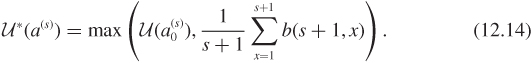
Let . One can show (see Problem 12.5) that

At the last stage, from equations (12.12) and (12.14) we obtain that and v(S) = 0. By backward induction on s it can be verified that (see Problem 12.5)

Therefore, from equations (12.14) and (12.16) at stage s, with x^(s) = 1

Let s* be the smallest positive integer so that (1/(S – 1) + ··· + 1/s) ≤ 1. The optimal procedure is to wait until s* offers are made. If the sth offer is the best so far far, accept it. Otherwise, wait until you reach the best offer so far and accept it. If you reach stage S you have to accept the offer irrespective of the rank. If S is large, s* ≈ S/e. So you should first just wait and observe approximately 1/e ≈ 36% of the offers. At that point the information-gathering stage ends and you accept the first offer that ranks above all previous offers.

Lindley (1961) provides a solution to this problem when the utility is linear in the rank, that is when u(θ) = S – θ.

12.4.2 The prophet inequality

This is an example discussed in Bather (2000). It has points in common with the one in the previous section. What it adds is a simple example of a so-called “prophet inequality”—a bound on the expected utility that can be expected if information that accrues sequentially was instead revealed in its entirety at the beginning.

You have the choice of one out of a set of S options. The values of the options are represented by nonnegative and independent random quantities θ⁽¹⁾, ..., θ^(S) with known probability distributions. Say you decided to invest a fixed amount of money for a year, and you are trying to choose among investment options with random returns. Let μ_s denote the expected return of option s, that is μ_s = E[θ^(s)], s = 1, ..., S. Assume that these means are finite, and assume that returns are in the utility scale.

Let us first consider two extreme situations. If you are asked to choose a single option now, your expected utility is maximized by choosing the option with largest mean, and that maximum is g_S = max(μ₁, ..., μ_S). At the other extreme, if you are allowed to communicate with a prophet that knows all the true returns, then your expected utility is h_S = E[max(θ⁽¹⁾, ..., θ^(S))]. Now, consider the sequential case in which you can ask the prophet about one option at the time. Suppose that the values of θ⁽¹⁾, ..., θ^(S) are revealed sequentially in this order. At each stage, you are only allowed to ask about the next option if you reject the ones examined so far. Cruel perhaps, but it makes for another interesting trade-off between learning and immediate gains.

At stage s, decisions can be , wait for the next offer, or , accept the offer and stop bothering the prophet. If you stop, your utility will be the value θ^(s) of the option you decided to accept. On the other hand, the expected utility of continuing . At the last stage, when there is only one option to be revealed, the expectation of the best utility that can be reached is , because is the only decision available. So when folding back to stage S – 1, you either accept option θ^(S−1) or wait to see θ^(S). That is, the maximum expected utility is U*^(S−1) = E[max(θ^(S−1), μ_S)] = E[max(θ^(S−1), U^*(S))]. With backward induction, we find that the expected maximum utility at stage s is

To simplify notation, let w_s denote the expected maximum utility when there are s options to consider, that is w_s = U^*(S−s+1), s = 1, ..., S. What is the advantage of obtaining full information of the options over the sequential procedure? We will prove the prophet’s inequality

This inequality is explained by Bather as follows:

Proof: To prove the inequality, first observe that w₁ = μ_S. Then, since w₂ = E[max(θ^(S−1), w₁)], it follows that w₂ ≥ E[θ^(S−1)] = μ_S−1 and w₂ ≥ w₁. Recursively, we can prove that the sequence w_s is increasing, that is

Define y₁ = θ⁽¹⁾ and y_r = max(θ^(r), w_r−1) for r = 2, ..., S. Moreover, define w₀ ≡ 0 and z_r = max(θ^(r) – w_r−1, 0). This implies that y_r = w_r−1 + z_r. From (12.20), w_r−1 ≤ w_S−1 for r = 1, ..., S. Thus,

For any r, it follows from our definitions that θ^(r) ≤ y_r. Thus,

By definition, z_r ≥ 0. Thus, max(z₁, ..., z_S) ≤ z₁ + ··· + z_S. By combining the latter inequality with that in (12.22), and taking expectations, we obtain

which completes the proof.

12.5 Sequential clinical trials

Our next set of illustrations, while still highly stylized, bring us far closer to real applications, particularly in the area of clinical trials. Clinical trials are scientific experiments on real patients, and involve the conflicting goals of learning about treatments, so that a broad range of patients may benefit from medical advances, and ensuring a good outcome for the patients enrolled in the trial. For a more general discussion on Bayesian sequential analysis of clinical trials see, for example, Berry (1987) and Berger and Berry (1988). While we will not examine this controversy in detail here, in the sequential setting the Bayesian and frequentist approaches can differ in important ways. Lewis and Berry (1994) discuss the value of sequential decision-theoretic approaches over conventional approaches. More specifically, they compare performances of Bayesian decision-theoretic designs to classical group-sequential designs of Pocock (1977) and O’Brien and Fleming (1979). This comparison is within the hypothesis testing framework in which the parameters associated with the utility function are chosen to yield classical type I and type II error rates comparable to those derived under the Pocock and O’Brien and Fleming designs. While the power functions of the Bayesian sequential decision-theoretic designs are similar to those of the classical designs, they usually have smaller-mean sample sizes.

12.5.1 Two-armed bandit problems

A decision maker can take a fixed number n of observations sequentially. At each stage, he or she can choose to observe either a random variable x with density f_x(.|θ₀) or a random variable y with f_y(.|θ₁). The decision problem is to find a sequential procedure that maximizes the expected value of the sum of the observations. This is an example of a two-armed bandit problem discussed in DeGroot (1970) and Berry and Fristedt (1985). For a clinical trial connection, imagine the two arms being two treatments for a particular illness, and the random variables being measures of well-being of the patients treated. The goal is to maximize the patient’s well-being, but some early experimentation is necessary on both treatments to establish how to best do so.

We can formalize the solution to this problem using dynamic programming. At stages s = 0, ..., n, the decision is either , observe x, or , observe y. Let π denote the joint prior distribution for θ = (θ₀, θ₁) and consider the maximum expected sum of the n observations given by

where , is calculated under distribution π.

Suppose the first observation is taken from x. The joint posterior distribution of (θ₀, θ₁) is π_x and the expected sum of the remaining (n – 1) observations is given by V⁽ⁿ⁻¹⁾(π_x). Then, the expected sum of all n observations is . Similarly, if the first observation comes from y, the expected sum of all n observations is . Thus, the optimal procedure a*_(n) has expected utility

With the initial condition that V⁽⁰⁾(π) ≡ 0, one can solve V^(s)(π), s = 1, ..., n, and find the sequential optimal procedure by induction.

12.5.2 Adaptive designs for binary outcomes

To continue in a similar vein, consider a clinical trial that compares two treatments, say A and B. Patients arrive sequentially, and each can only receive one of the two therapies. Therapy is chosen on the basis of the information available up until that point on the treatments’ efficacy. Let n denote the total number of patients in the trial. At the end of the trial, the best-looking therapy is assigned to (N – n) additional patients. The total number N of patients involved is called the patient horizon. A natural question in this setting is how to optimally allocate patients in the trial to maximize the number of patients who respond positively to the treatment over the patient horizon N. This problem is solved with dynamic programming.

Let us say that response to treatment is a binary event, and call a positive response simply “response.” Let θ_A and θ_B denote the population proportion of responses under treatments A and B, respectively. For a prior distribution, assume that θ_A and θ_B are independent and with a uniform distribution on (0, 1). Let n_A denote the number of patients assigned to treatment A and r_A denote the number of responses among those n_A patients. Similarly, define n_B and r_B for treatment B.

To illustrate the required calculations, assume n = 4 and N = 100. When using dynamic programming in the last stage, we need to consider all possibilities for which n_A + n_B = n = 4. Consider for example n_A = 3 and n_B = 1. Under this configuration, r_A takes values in 0, ..., 3 while r_B takes values 0 or 1. Consider n_A = 3, r_A = 2, n_B = 1, r_B = 0. The posterior distribution of θ_A is Beta(3, 2) and the predictive probability of response is 3/5, while θ_B is Beta(1, 2) with predictive probability 1/3. Because 3/5 > 1/3 the remaining N – n = 100 – 4 = 96 patients are assigned to A with an expected number of responses given by 96 × 3/5 = 57.6. Similar calculations can be carried out for all other combinations of treatment allocations and experimental outcomes.

Next, take one step back and consider the cases in which n_A + n_B = 3. Take n_A = 2, n_B = 1 for an example. Now, r_A takes values 0, 1, or 2 while r_B takes values 0 or 1. Consider the case n_A = 2, r_A = 1, n_B = 1, r_B = 0. The current posterior distributions are Beta(2, 2) for θ_A and Beta(1, 2) for θ_B. If we are allowed one additional observation in the trial before we get to n = 4, to calculate the expected number of future responses we need to consider two possibilities: assigning the last patient to treatment A or to treatment B.

Choosing A moves the process to the case n_A = 3, n_B = 1. If the patient responds, r_A = 2, r_B = 0 with predictive probability 2/4 = 1/2. Otherwise, with probability 1/2, the process moves to the case r_A = 1, r_B = 0. The maximal number of responses is 57.6 (as calculated above) with probability 1/2 and 38.4 (this calculation is omitted and left as an exercise) with probability 1/2. Thus, the expected number of future responses with A is (1 + 57.6) × 1/2 + 38.4 × 1/2 = 48.5. Similarly, when treatment B is chosen for the next patient n_A = 2, n_B = 2. If the patient responds to treatment B, which happens with probability 1/3, the process moves to r_A = 1, r_B = 1; otherwise it moves to r_A = 1, r_B = 0. One can show that the expected number of successes under treatment B is 48.3. Because 48.5 > 48.3, the optimal decision is to assign the next patient to treatment A.

After calculating the maximal expected number of responses for all cells under which n_A + n_B = 3, we turn to the case with n_A + n_B = 2 and so on until n_A + n_B = 0. Figure 12.6 shows the optimal decisions when n = 4 and N = 100 for each combination of n_A, r_A, n_B, r_B. Each separated block of cells corresponds to a pair (n_A, n_B). Within each block, each individual cell is a combination of r_A = 0, ..., n_A and r_B = 0, ..., n_B. In the figure, empty square boxes denote cases for which A is the optimal decision while full square boxes denote cases for which B is optimal. An asterisk represents cases where both treatments are optimal. For instance, the left bottom corner of the figure has n_A = r_A = 0, n_B = r_B = 0, for which both treatments are optimal. Then, in the top left block of cells when n_A = r_A = 0 and n_B = 4, the optimal treatment is A for r_B = 0, 1. Otherwise, B is optimal. Figure 12.7 shows the optimal design under two different prior choices on θ_A. These priors were chosen to have mean 0.5, but different variances.

Figure 12.6 Optimal decisions when n = 4 and N = 100 given available data as given by n_A,r_A, n_B, and r_B.

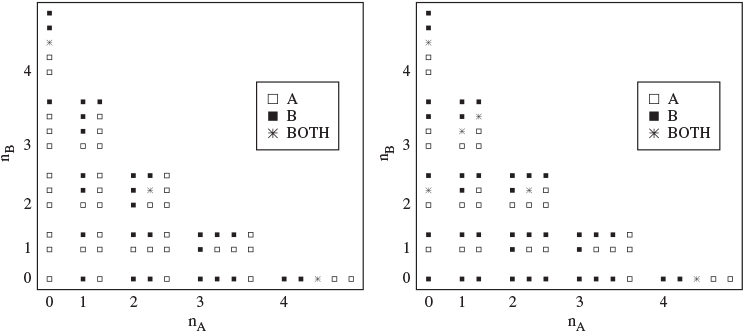
Figure 12.7 Sensitivity of the optimal decisions under two different prior choices for θ_A when n = 4 and N = 100. Designs shown in the left panel assume that θ_A ~ Beta(0.5, 0.5). In the right panel we assume θ_A ~ Beta(2, 2).

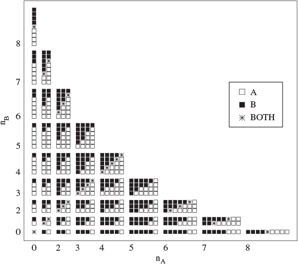
Figure 12.8 Optimal decisions when n = 8 and N = 100 given available data as given by n_A, r_A, n_B, and r_B.

In Figure 12.8 we also show the optimal design when n = 8 and N = 100 assuming independent uniform priors for θ_A and θ_B, while in Figure 12.9 we give an example of the sensitivity of the design to prior choices on θ_A. Figures in this section are similar to those presented in Berry and Stangl (1996, chapter 1).

Figure 12.9 Sensitivity of the optimal decisions under two different prior choices for θ_A when n = 8, N = 100. Designs shown in the left panel assume that θ_A ~ Beta(0.5, 0.5). In the right panel we assume θ_A ~ Beta(2, 2).

In the example we presented, the allocation of patients to treatments is adaptive, in that it depends on the results of previous patients assigned to the same treatments. This is an example of an adaptive design. Berry and Eick (1995) discuss the role of adaptive designs in clinical trials and compare some adaptive strategies to balanced randomization which has a traditional and dominant role in randomized clinical trials. They conclude that the Bayesian decision-theoretic adaptive design described in the above example (assuming that θ_A and θ_B are independent and with uniform distributions) is better for any choice of patient horizon N. However, when the patient horizon is very large, this strategy does not perform much better than balanced randomization. In fact, balanced randomization is a good solution when the aim of the design is maximizing effective treatment in the whole population. However, if the condition being treated is rare then learning with the aim of extrapolating to a future population is much less important, because the future population may not be large. In these cases, using an adaptive procedure is more critical.

12.6 Variable selection in multiple regression

We now move to an application to multiple regression, drawn from Lindley (1968a). Let y denote a response variable, while x = (x₁, ..., x_p)′ is vector of explanatory variables. The relationship between y and x is governed by

E[y|θ,x] =	x′θ
Var[y|θ,x] =	σ2;

that is, we have a linear multiple regression model with constant variance. To simplify our discussion we assume that σ² is known. We make two additional assumptions. First, we assume that θ and x are independent, that is

f(x, θ) = f(x)π(θ).

This means that learning the value of the explanatory variables alone does not carry any information about the regression coefficients. Second, we assume that y has known density f(y|x, θ), so that we do not learn anything new about the likelihood function from new observations of either x or y.

The decision maker has to predict a future value of the dependent variable y. To help with the prediction he or she can observe some subset (or all) of the p explanatory variables. So, the questions of interest are: (i) which explanatory variables should the decision maker choose; and (ii) having observed the explanatory variables of his or her choice, what is the prediction for y?

Let I denote the subset of integers in the set {1, ..., p} and J denote the complementary subset. Let x^I denote a vector with components x_i, i ∊ I. Our decision space consists of elements a = (I, g(.)) where g is a function from ℜ^s to ℜ; that is, it consists of a subset of explanatory variables and a prediction function. Let us assume that our loss function is

u(a(θ)) = −(y – g(x^I))² – c_I;

that is, we have a quadratic utility for the prediction g(x^I) for y with a cost c_I for observing explanatory variables with indexes in I. This allows different variables to have different costs.

Figure 12.10 shows the decision tree for this problem. At the last stage, we consider the expected utility, for fixed x^I, averaging over y, that is we compute

Next, we select the prediction g(x^I) that maximizes equation (12.26). Under the quadratic utility function, the optimal prediction is given by

Figure 12.10 Decision tree for selecting variables with the goal of prediction. Figure adapted from Lindley (1968a).

The unknowns in this prediction problem include both the parameters and the unobserved variables. Thus

that is, to obtain the optimal prediction we first estimate the unobserved explanatory variables x^J and combine those with the observed x^I and the estimated regression parameters.

Folding back the decision tree, by averaging over x^I for fixed I, we obtain

E[(y – E[x|xI]′ E[θ])2] =	σ2 + E[x′θ – E[x|xI]′ E[θ]]2
=	σ2 + tr(Var[θ]Var[x]) + E[x]′ Var[θ]E[x]
	+ E[θ]′ Var[xJ]E[θ]

where Var[θ] and Var[x] are the covariance matrices for θ and x, respectively, and Var[x^J] = E[(x – E[x|x^I])(x – E[x|x^I]′)], that is the covariance matrix of the whole predictor vector, once the subset x^I is fixed.

Thus, the expected utility for fixed I is

The optimal solution at the first stage of the decision tree is obtained by maximizing equation (12.28) over I. Because only the last two elements of equation (12.28) depend on I, this corresponds to choosing I to reach

The solution will depend both on how well the included and excluded x predict y, and on how well the included x^I predict the excluded x^J.

As a special case, suppose that the costs of each observation x_i, i ∊ I, are additive so that . Moreover, assume that the explanatory variables are independent. This implies

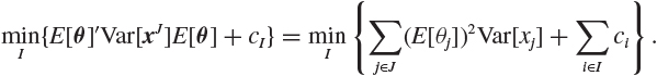
It follows from the above equation that x_i should be observed if and only if

(E[θ_i])²Var[x_i] > c_i;

Figure 12.11 Decision tree for selecting variables with the goal of controlling the response. Figure adapted from Lindley (1968a).

that is, if either its variation is large or the squared expected value of the regression parameter is large compared to the cost of observation.

Let us now change the decision problem and assume that we can set the explanatory variables as we want, and the goal is to bring the value of the response variable towards a preassigned value y₀. The control of the response variable depends on the selection of explanatory variables and on the choice of a setting . Our decision space consists of elements a = (I, x^I); that is, it consists of selecting a subset of explanatory variables and the values assigned to these variables. Let us assume that our utility function is

u(a(θ)) = −(y – y₀)² – c(x^I).

This is no longer a two-stage sequential decision problem, because no new data are accrued between the choice of the subset and the choice of the setting. As seen in Figure 12.11 this is a nested decision problem, and it can be solved by solving for the setting given I, and plugging the solution back into the expected utility to solve for I. In a sense, this is a special case of dynamic programming where we skip one of the expectations. Using additional assumptions on the distributions of x and on the form of the cost function, in a special case Lindley (1968a) shows that if y₀ = 0 and the cost function does not depend on x^I, then an explanatory variable x_i is chosen for controlling if and only if

This result parallels that seen earlier. However, a point of contrast is that the decision depends on the variance, rather than the mean, of the regression parameter, as a result of the differences in goals for the decision making. For a detailed development see Lindley (1968a).

12.7 Computing

Implementation of the fully sequential decision-theoretic approach is challenging in applications. In addition to the general difficulties that apply with the elicitation of priors and utilities in decision problems, the implementation of dynamic programming is limited by its computational complexity that grows exponentially with the maximum number of stages S. In this section we review a couple of examples that give a sense of the challenges and possible approaches.

Suppose one wants to design a clinical trial to estimate the effect θ of an experimental treatment over a placebo. Prior information about this parameter is summarized by π(θ) and the decisions are made sequentially. There is a maximum of S times, called monitoring times, when we can examine the data accrued that far, and take action. Possible actions are a₁ (stop the trial and conclude that the treatment is better), a₂ (stop the trial and conclude that the placebo is preferred), or a₃ (continue the trial). At the final monitoring time S, the decision is only between actions a₁ and a₂ with utility functions

with y₊ = max(0, y). This utility builds in an indifference zone (b₂, b₁) within which the effect of the treatment is considered similar to that of placebo and, thus, either is acceptable. Low θ are good (say, they imply a low risk) so the experimental treatment is preferred when θ < b₂, while placebo is preferred when θ > b₁. Also, suppose a constant cost C for any additional observation.

As S increases, backwards induction becomes increasingly computationally diffi-cult. Considering the two-sided sequential decision problem described above, Carlin et al. (1998) propose an approach to reduce the computational complexity associated with dynamic programming. Their forward sampling algorithm can be used to find optimal stopping boundaries within a class of decision problems characterized by decision rules of the form

E[θ|x(1), ..., x(s)] ≤ γs,L	choose a1
E[θ|x(1), ..., x(s)] > γs,U	choose a2
γs,L < E[θ|x(1), ..., x(s)] ≤ γs,U	choose a3

for s = 1, ..., S and with γ_S,L = γ_S,U = γ_S.

To illustrate how their method works, suppose that S = 2 and that a cost C is associated with carrying out each stage of the trial. To determine a sequential decision rule of the type considered here, we need to specify a total of (2S – 1) decision boundaries. Let

γ = (γ_S−2,L, γ_S−2,U, γ_S−1,L, γ_S−1,U, γ_S)′

denote the vector of these boundaries. To find an optimal γ we first generate a Monte Carlo sample of size M from f(θ, x^(S−1), x^(S)) = π(θ)f(x^(S−1)|θ)f(x^(S)|θ). Let denote a generic element in the sample. For a fixed γ, the utilities achieved with this rule are calculated using the following algorithm:

A Monte Carlo estimate of the posterior expected utility incurred with γ is given by

This algorithm provides a way of evaluating the expected utility of any strategy, and can be embedded into a (2S – 1)-dimensional optimization to numerically search for the optimal decision boundary γ *. With this procedure Carlin et al. (1998) replace the initial decision problem of deciding among actions a₁, a₂, a₃ by a problem in which one needs to find optimal thresholds that define the stopping times in the sequential procedure. The strategy depends on the history of actions and observations only through the current posterior mean. The main advantage of the forward sampling algorithm is that it grows only linearly in S, while the backward induction algorithm would grow exponentially with S. A disadvantage is that it requires a potentially difficult maximization over a continuous space of dimension (2S – 1), while dynamic programming is built upon simple one-dimensional discrete maximizations over the set of actions.

Kadane and Vlachos (2002) consider a hybrid algorithm which combines dynamic programming with forward sampling. Their hybrid algorithm works backwards for S₀ stages and provides values of the expected utility for the optimal continuation. Then, the algorithm is completed by forward sampling from the start of the trial up to the stage S₀ when backward induction starts. While reducing the optimization problem with forward sampling, the hybrid algorithm allows for a larger number of stages in sequential problems previously intractable with dynamic programming. The trade-off between accuracy in the search for optimal strategies and computing time is controlled by the maximum number of backward induction steps S₀.

Müller et al. (2007a) propose a combination of forward simulation, to approximate the integral expressions, and a reduction of the allowable action space and sample space, to avoid problems related to an increasing number of possible trajectories in the backward induction. They also assume that at each stage, the choice of an action depends on the data portion of the history set H_s−1 only through a function T_s of H_s−1. This function could potentially be any summary statistic, such as the posterior mean as in Carlin, Kadane & Gelfand (1998). At each stage s, both T_s−1 and a^(s−1) are discretized over a finite grid. Evaluation of the expected utility uses forward sampling. M samples (θ_m, x_m) are generated from the distribution f(x⁽¹⁾, ..., x^(S−1)|θ)π(θ). This is done once for all, and stretching out the data generation to its maximum number of stages, irrespective of whether it is optimal to stop earlier or not. The value of the summary statistic T_s,m is then recorded at stage 1 through S – 1 for every generated data sequence. The coarsening of data and decisions to a grid simplifies the computation of the expected utilities, which are now simple sums over the set of indexes m that lead to trajectories that belong to a given cell in the history. As the grid size is kept constant, the method avoids the increasing number of pathways with the traditional backward induction. This constrained backward induction is an approximate method and its successful implementation depends on the choice of the summary statistic T_s, the number of points on the grid for T_s, and the number M of simulations. An application of this procedure to a sequential dose-finding trial is described in Berry et al. (2001).

Brockwell and Kadane (2003) also apply discretization of well-chosen statistics to simplify the history H_s. Their examples focus on statistics of dimension up to three and a maximum of 50 stages. They note, however, that sequential problems involving statistics with higher dimension may be still intractable with the gridding method. More broadly, computational sequential analysis is still an open area, where novel approaches and progress could greatly contribute to a more widespread application of the beautiful underlying ideas.

12.8 Exercises

Problem 12.1 (French 1988) Four well-shuffled cards, the kings of clubs, diamonds, hearts, and spades, are laid face down on the table. A man is offered the following choice. Either: a randomly selected card will be turned over. If it is red, he will win £100; if it is black, he will lose £100. Or: a randomly selected card will be turned over. He may then choose to pay £35 and call the bet off or he may continue. If he continues, one of the remaining three cards will be randomly selected and turned over. If it is red, he will win £100; if it is black, he will lose £100. Draw a decision tree for the problem. If the decision maker is risk neutral, what should he do? Suppose instead that his utility function for sums of money in this range is u(x) = log(1 + x/200). What should he do in this case?

Problem 12.2 (French 1988) A builder is offered two plots of land for house building at £20 000 each. If the land does not suffer from subsidence, then he would expect to make £10 000 net profit on each plot, when a house is built on it. However, if there is subsidence, the land is only worth £2000 so he would make an £18 000 loss. He believes that the chance that both plots will suffer from subsidence is 0.2, the chance that one will suffer from subsidence is 0.3, and the chance that neither will is 0.5. He has to decide whether to buy the two plots or not. Alternatively, he may buy one, test it for subsidence, and then decide whether to buy the other plot. Assuming that the test is a perfect predictor of subsidence and that it costs £200 for the test, what should he do? Assume that his preferences are determined purely by money and that he is risk neutral.

Problem 12.3 (French 1988) You have decided to buy a car, and have eliminated possibilities until you are left with a straight choice between a brand new car costing £4000 and a second-hand car costing £2750. You must have a car regularly for work. So, if the car that you buy proves unreliable, you will have to hire a car while it is being repaired. The guarantee on the new car covers both repair costs and hire charges for a period of two years. There is no guarantee on the second-hand car. You have considered the second-hand-car market and noticed that cars tend to be either very good buys or very bad buys, few cars falling between the two extremes. With this in mind you consider only two possibilities.

1. The second-hand car is a very good buy and will involve you in £750 expenditure on car repairs and car hire over the next two years.

2. The second-hand car is a very bad buy and will cost you £1750 over the next two years.

You also believe that the probability of its being a good buy is only 0.25. However, you may ask the AA for advice at negligible financial cost, but risking a probability of 0.3 that the second-hand car will be sold while they are arranging a road test. The road test will give a satisfactory or unsatisfactory report with the following probabilities:

Probability of AA report being:	Conditional on the car being:
	a very bad buy	a very good buy
Satisfactory	0.1	0.9
Unsatisfactory	0.9	0.1

If the second-hand car is sold before you buy it, you must buy the new car. Alternatively you may ask your own garage to examine the second-hand car. They can do so immediately, thus not risking the loss of the option to buy, and will also do so at negligible cost, but you do have to trust them not to take a “back-hander” from the second-hand-car salesman. As a result, you evaluate their reliability as:

Probability of garage report being:	Conditional on the car being:
	a very bad buy	a very good buy
Satisfactory	0.5	1
Unsatisfactory	0.5	0

You can arrange at most one of the tests. What should you do, assuming that you are risk neutral for monetary gains and losses and that no other attribute is of importance to you?

Problem 12.4 Write the algorithm of Section 12.3.2 for the case in which z only depends on the unknown θ and the terminal action, and in which observation of each of the random variables in stages 1, ..., S – 1 has cost C.

Problem 12.5 Referring to Section 12.4.1:

1. Prove equation (12.15).

2. Use backwards induction to prove equation (12.16).

Problem 12.6 Consider the example discussed in Section 12.4.2. Suppose that θ⁽¹⁾, ..., θ^(S) are independent and identically distributed with a uniform distribution on [0, 1]. Prove that