3.3. Optimality Conditions

Search in book...
Toggle Font Controls
Create new playlist

Name your new playlist

Playlist description (optional)
Sign In

Email address

Password

Forgot Password?

or

Continue with Facebook

Continue with Google
Sign Up

Full Name

Email address

Confirm Email Address

Password

or

Continue with Facebook

Continue with Google

3.3. Optimality Conditions

A basic knowledge of optimality conditions is important for understanding the performance of the various numerical methods discussed later in the chapter. In this section, we introduce the basic concept of optimality, the necessary and sufficient conditions for the relative maxima and minima of a function, as well as the solution methods based on the optimality conditions. Simple examples are used to explain the underlying concepts. The examples will also show the practical limitations of the methods.

3.3.1. Basic Concept of Optimality

We start by recalling a few basic concepts we learned in Calculus regarding maxima and minima, followed by defining local and global optima; thereafter, we illustrate the concepts using functions of one and multiple variables.

3.3.1.1. Functions of a single variable

This section presents a few definitions for basic terms.

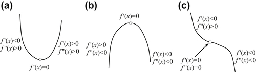
Stationary point: For a continuous and differentiable function f(x), a stationary point x^∗ is a point at which the slope of the function vanishes—that is, f ′(x) = df/dx = 0 at x = x^∗, where x^∗ belongs to its domain of definition. As illustrated in Figure 3.7, a stationary point can be a minimum if f ″(x) > 0, a maximum if f ″(x) < 0, or an inflection point if f ″(x) = 0 in the neighborhood of x^∗.

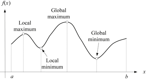
FIGURE 3.7 A stationary point may be (a) a minimum, (b) a maximum, or (c) an inflection point.

FIGURE 3.8 Global and local minimum of a function f(x).

Global and local minimum: A function f(x) is said to have a local (or relative) minimum at x = x^∗ if f(x^∗) ≤ f(x^∗ + δ) for all sufficiently small positive and negative values of δ, that is, in the neighborhood of the point x∗. A function f(x) is said to have a global (or absolute) minimum at x = x∗ if f(x∗) ≤ f(x) for all x in the domain over which f(x) is defined. Figure 3.8 shows the global and local optimum points of a function f(x) with a single variable x.

Necessary condition: Consider a function f(x) of single variable defined for a < x < b. To find a point of x^∗∈(a, b) that minimizes f(x), the first derivative of function f(x) with respect to x at x = x^∗ must be a stationary point; that is, f ′(x^∗) = 0.

Sufficient condition: For the same function f(x) stated above and f ′(x^∗) = 0, then it can be said that f(x^∗) is a minimum value of f(x) if f ″(x^∗) > 0, or a maximum value if f ″(x^∗) < 0.

EXAMPLE 3.1

Find a minimum of the function f(x) = x² − 2x, for x ∈ (0, 2).

Solutions

The first derivative of f(x) with respect to x is f ′(x) = 2x − 2. We set f ′(x) = 0, and solve for x = 1, which is a stationary point. This is the necessary condition for x = 1 to a minimum of the function f(x).

We take second derivative of f(x) with respect to x, f ″(x) = 2 > 0, which satisfies the sufficient condition of the function f(x) that has a minimum at x = 1, and the minimum value of the function at x = 1 is f(1) = −1.

The concept illustrated above can be easily extended to functions of multiple variables. We use functions of two variables to provide a graphical illustration on the concepts.

3.3.1.2. Functions of multiple variables

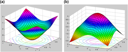
A function of two variables f(x₁, x₂) = −(cos²x₁ + cos²x₂)² is graphed in Figure 3.9a. Perturbations from point (x₁, x₂) = (0, 0), which is a local minimum, in any direction result in an increase in the function value of f(x); that is, the slopes of the function with respect to x₁ and x₂ are zero at this point of local minimum. Similarly, a function f(x₁, x₂) = (cos²x₁ + cos²x₂)² graphed in Figure 3.9b has a local maximum at (x₁, x₂) = (0, 0). Perturbations from this point in any direction result in a decrease in the function value of f(x); that is, the slopes of the function with respect to x₁ and x₂ are zero at this point of local maximum. The first derivatives of the function with respect to the variables are zero at the minimum or maximum, which again is called a stationary point.

Necessary condition: Consider a function f(x) of multivariables defined for x ∈ Rⁿ, where n is the number of variables. To find a point of x^∗ ∈ Rⁿ that minimizes f(x), the gradient of the function f(x) at x = x^∗ must be a stationary point; that is, ∇f(x^∗) = 0.

The gradient of a function of multivariables is defined as

$\nabla f (x) \equiv {[\frac{\partial f}{\partial x_{1}}, \frac{\partial f}{\partial x_{2}}, ..., \frac{\partial f}{\partial x_{n}}]}^{T}$ $\nabla f (x) \equiv {[\frac{\partial f}{\partial x_{1}}, \frac{\partial f}{\partial x_{2}}, ..., \frac{\partial f}{\partial x_{n}}]}^{T}$

(3.8)

Geometrically, the gradient vector is normal to the tangent plane at a given point x, and it points in the direction of maximum increase in the function. These properties are quite important; they will be used in developing optimality conditions and numerical methods for optimum design. In Example 3.2, the gradient vector for a function of two variables is calculated for illustration purpose.

FIGURE 3.9 Functions of two variables (MATLAB Script 2 can be found in Appendix A): (a) f(x₁, x₂) = −(cos²x₁ + cos²x₂)² with a local minimum at (0, 0) and (b) f(x₁, x₂) = (cos²x₁ + cos²x₂)² with a local maximum at (0, 0).

EXAMPLE 3.2

A function of two variables is defined as

$f (x_{1}, x_{2}) = x_{2} e^{- x_{1}^{2} - x_{2}^{2}}$ $f (x_{1}, x_{2}) = x_{2} e^{- x_{1}^{2} - x_{2}^{2}}$

(3.9a)

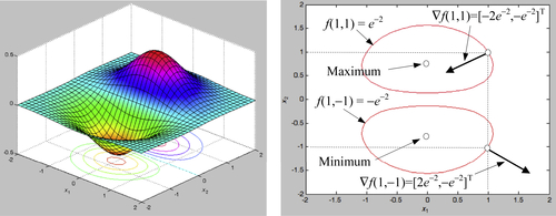
which is graphed in MATLAB shown below (left). The MATLAB script for the graph can be found in Appendix A (Script 3). Calculate the gradient vectors of the function at (x₁, x₂) = (1, 1) and (x₁, x₂) = (1,−1).

Solutions

From Eq. 3.8, the gradient vector of the function f(x₁, x₂) is

$\nabla f (x_{1}, x_{2}) = {[- 2 x_{1} x_{2} e^{- x_{1}^{2} - x_{2}^{2}}, e^{- x_{1}^{2} - x_{2}^{2}} - 2 x_{2}^{2} e^{- x_{1}^{2} - x_{2}^{2}}]}^{T}$ $\nabla f (x_{1}, x_{2}) = {[- 2 x_{1} x_{2} e^{- x_{1}^{2} - x_{2}^{2}}, e^{- x_{1}^{2} - x_{2}^{2}} - 2 x_{2}^{2} e^{- x_{1}^{2} - x_{2}^{2}}]}^{T}$

(3.9b)

At (x₁, x₂) = (1, 1), f(1, 1) = e⁻² = 0.1353, and ∇f(1, 1) = [−2e⁻², −e⁻²]^T; and at (x₁, x₂) = (1,−1), f(1,−1) = −e⁻² = −0.1353, and ∇f(1, −1) = [2e⁻², −e⁻²]^T. The iso-lines of f(1, 1) and f(1, −1) as well as the gradient vectors at (1, 1) and (1,−1) are shown in the figure below (right). In this example, gradient vector at a point x is perpendicular to the tangent line at x, and the vector points in the direction of maximum increment in the function value. The maximum and minimum of the function are shown for clarity.

Sufficient condition: For the same function f(x) stated above, let ∇f(x^∗) = 0, then f(x^∗) has a minimum value of f(x) if its Hessian matrix defined in Eq. 3.10 is positive-definite.

$H = \nabla^{2} f = [\frac{\partial^{2} f}{\partial x_{i} \partial x_{j}}] = {[\begin{matrix} \frac{\partial^{2} f}{{\partial x}_{1}^{2}} & \frac{\partial^{2} f}{{\partial x}_{1} \partial x_{2}} & ... & \frac{\partial^{2} f}{{\partial x}_{1} \partial x_{n}} \\ \frac{\partial^{2} f}{{\partial x}_{2} \partial x_{1}} & \frac{\partial^{2} f}{{\partial x}_{2}^{2}} & ... & \frac{\partial^{2} f}{{\partial x}_{2} \partial x_{n}} \\ ... & ... & ... \\ \frac{\partial^{2} f}{{\partial x}_{n} \partial x_{1}} & \frac{\partial^{2} f}{{\partial x}_{n} \partial x_{2}} & ... & \frac{\partial^{2} f}{{\partial x}_{n}^{2}} \end{matrix}]}_{n \times n}$ $H = \nabla^{2} f = [\frac{\partial^{2} f}{\partial x_{i} \partial x_{j}}] = {[\begin{matrix} \frac{\partial^{2} f}{{\partial x}_{1}^{2}} & \frac{\partial^{2} f}{{\partial x}_{1} \partial x_{2}} & ... & \frac{\partial^{2} f}{{\partial x}_{1} \partial x_{n}} \\ \frac{\partial^{2} f}{{\partial x}_{2} \partial x_{1}} & \frac{\partial^{2} f}{{\partial x}_{2}^{2}} & ... & \frac{\partial^{2} f}{{\partial x}_{2} \partial x_{n}} \\ ... & ... & ... \\ \frac{\partial^{2} f}{{\partial x}_{n} \partial x_{1}} & \frac{\partial^{2} f}{{\partial x}_{n} \partial x_{2}} & ... & \frac{\partial^{2} f}{{\partial x}_{n}^{2}} \end{matrix}]}_{n \times n}$

(3.10)

where all derivatives are calculated at the given point x^∗. The Hessian matrix is an n × n matrix, where n is the number of variables. It is important to note that each element of the Hessian is a function in itself that is evaluated at the given point x^∗. Also, because f(x) is assumed to be twice continuously differentiable, the cross partial derivatives are equal; that is,

$\frac{\partial^{2} f}{\partial x_{i} \partial x_{j}} = \frac{\partial^{2} f}{\partial x_{j} \partial x_{i}}; i, j = 1, n$ $\frac{\partial^{2} f}{\partial x_{i} \partial x_{j}} = \frac{\partial^{2} f}{\partial x_{j} \partial x_{i}}; i, j = 1, n$

(3.11)

Therefore, the Hessian is always a symmetric matrix. The Hessian matrix plays a prominent role in exploring the sufficiency conditions for optimality.

Note that a square matrix is positive-definite if (a) the determinant of the Hessian matrix is positive (i.e., |H| > 0) or (b) all its eigenvalues are positive. To calculate the eigenvalues λ of a square matrix, the following equation is solved:

$| H - λ I | = 0$ $| H - λ I | = 0$

(3.12)

where I is an identity matrix of n × n.

EXAMPLE 3.3

A function of three variables is defined as

$f (x_{1}, x_{2}, x_{2}) = x_{1}^{2} + 2 x_{1} x_{2} + 2 x_{2}^{2} + x_{3}^{2} - 2 x_{1} + x_{2} + 8$ $f (x_{1}, x_{2}, x_{2}) = x_{1}^{2} + 2 x_{1} x_{2} + 2 x_{2}^{2} + x_{3}^{2} - 2 x_{1} + x_{2} + 8$

(3.13a)

Calculate the gradient vector of the function and determine a stationary point, if it exists. Calculate a Hessian matrix of the function f, and determine if the stationary point found gives a minimum value of the function f.

Solutions

We first calculate the gradient of the function and set it to zero to find the stationary point(s), if any:

$\nabla f (x_{1}, x_{2}, x_{3}) = {[2 x_{1} + 2 x_{2} - 2, 2 x_{1} + 4 x_{2} + 1, 2 x_{3}]}^{T}$ $\nabla f (x_{1}, x_{2}, x_{3}) = {[2 x_{1} + 2 x_{2} - 2, 2 x_{1} + 4 x_{2} + 1, 2 x_{3}]}^{T}$

(3.13b)

Setting Eq. 3.13b to zero, we have x = [2.5, −1.5, 0]^T, which is the only stationary point. Now, we calculate the Hessian matrix:

$H = \nabla^{2} f = [\begin{matrix} 2 & 2 & 0 \\ 2 & 4 & 0 \\ 0 & 0 & 1 \end{matrix}]$ $H = \nabla^{2} f = [\begin{matrix} 2 & 2 & 0 \\ 2 & 4 & 0 \\ 0 & 0 & 1 \end{matrix}]$

(3.13c)

which is positive-definite because

$| H | = | \begin{matrix} 2 & 2 & 0 \\ 2 & 4 & 0 \\ 0 & 0 & 1 \end{matrix} | = 8 - 4 = 4 > 0$ $| H | = | \begin{matrix} 2 & 2 & 0 \\ 2 & 4 & 0 \\ 0 & 0 & 1 \end{matrix} | = 8 - 4 = 4 > 0$

(3.13d)

$| H - λ I | = | \begin{matrix} 2 - λ & 2 & 0 \\ 2 & 4 - λ & 0 \\ 0 & 0 & 1 - λ \end{matrix} | = (2 - λ) (4 - λ) (1 - λ) - 4 (1 - λ) = 0$ $| H - λ I | = | \begin{matrix} 2 - λ & 2 & 0 \\ 2 & 4 - λ & 0 \\ 0 & 0 & 1 - λ \end{matrix} | = (2 - λ) (4 - λ) (1 - λ) - 4 (1 - λ) = 0$

(3.13e)

Solving Eq. 3.13e, we have λ = 1, 0.7639 and 5.236, which are all positive. Hence, the Hessian matrix is positive-definite; therefore, the stationary point x∗ = [2.5, −1.5, 0]^T is a minimum point, at which the function value is f(x∗) = 4.75.

3.3.2. Basic Concept of Design Optimization

For an optimization problem defined in Eq. 3.3, we find design variable vector x to minimize an objective function f(x) subject to the inequality constraints g_i(x) ≤ 0, i = 1 to m, the equality constraints h_j(x) = 0, j = 1 to p, and the side constraints x_k^ℓ ≤ x_k ≤ x_k^u, k = 1, n. In Eq. 3.5, we define the feasible set S, or feasible region, for a design problem as a collection of feasible designs. For unconstrained problems, the entire design space is feasible because there are no constraints. In general, the optimization problem is to find a point in the feasible region that gives a minimum value to the objective function. From a design perspective, in particular solving Eq. 3.3, we state the followings terms.

Global minimum: A function f(x) of n design variables has a global minimum at x^∗ if the value of the function at x^∗ ∈ S is less than or equal to the value of the function at any other point x in the feasible set S. That is,

$f (x^{*}) \leq f (x), \forall (for all) x \in S$ $f (x^{*}) \leq f (x), \forall (for all) x \in S$

(3.14)

If strict inequality holds for all x other than x^∗ in Eq. 3.14, then x^∗ is called a strong (strict) global minimum; otherwise, it is called a weak global minimum.

Local minimum: A function f(x) of n design variables has a local (or relative) minimum at x^∗ ∈ S if inequality of Eq. 3.14 holds for all x in a small neighborhood N (vicinity) of x^∗. If strict inequality holds, then x^∗ is called a strong (strict) local minimum; otherwise, it is called a weak local minimum.

Neighborhood N of point x^∗ is defined as the set of points:

$N = {x | x \in S with ‖ x - x^{*} ‖ < δ}$ $N = {x | x \in S with ‖ x - x^{*} ‖ < δ}$

(3.15)

for some small δ > 0. Geometrically, it is a small feasible region around point x^∗, such as a sphere of radius δ for n = 3 (number of design variables n = 3).

Next, we illustrate the derivation of the necessary and sufficient conditions using Taylor's series expansion. For the time being, we assume unconstrained problems. In the next subsection, we extend the discussion to constrained problems.

Expanding the objective function f(x) at the inflection point x^∗ using Taylor's series, we have

$f (x) = f (x^{*}) + \nabla f {(x^{*})}^{T} Δ x + \frac{1}{2} Δ x^{T} H (x^{*}) Δ x + R$ $f (x) = f (x^{*}) + \nabla f {(x^{*})}^{T} Δ x + \frac{1}{2} Δ x^{T} H (x^{*}) Δ x + R$

(3.16)

where R is the remainder containing higher-order terms in Δx, and Δx = x − x^∗. We define increment Δf(x) as

$Δ f (x) = f (x) - f (x^{*}) = \nabla f {(x^{*})}^{T} Δ x + \frac{1}{2} Δ x^{T} H (x^{*}) Δ x + R$ $Δ f (x) = f (x) - f (x^{*}) = \nabla f {(x^{*})}^{T} Δ x + \frac{1}{2} Δ x^{T} H (x^{*}) Δ x + R$

(3.17)

If we assume a local minimum at x^∗, then Δf must be nonnegative due to the definition of a local minimum given in Eq. 3.14; that is, Δf ≥ 0.

Because Δx is small, the first-order term ∇f(x^∗)^T Δx dominates other terms, and therefore Δf can be approximated as Δf(x) = ∇f(x^∗)^TΔx. Note that Δf in this equation can be positive or negative depending on the sign of the term ∇f(x^∗)^TΔx. Because Δx is arbitrary (a small increment in x^∗), its components may be positive or negative. Therefore, we observe that Δf can be nonnegative for all possible Δx unless

$\nabla f (x^{*}) = 0$ $\nabla f (x^{*}) = 0$

(3.18)

In other words, the gradient of the function at x^∗ must be zero. In the component form, this necessary condition becomes

$\frac{\partial f (x^{*})}{\partial x_{i}} = 0, i = 1, n$ $\frac{\partial f (x^{*})}{\partial x_{i}} = 0, i = 1, n$

(3.19)

Again, points satisfying Eq. 3.18 or Eq. 3.19 are called stationary points.

Considering the second term on the right-hand side of Eq. 3.17 evaluated at a stationary point x^∗, the positivity of Δf is assured if

$Δ x^{T} H (x^{*}) Δ x > 0$ $Δ x^{T} H (x^{*}) Δ x > 0$

(3.20)

for all Δx ≠ 0. This is true if the Hessian H(x^∗) is a positive-definite matrix, which is then the sufficient condition for a local minimum of f(x) at x^∗.

3.3.3. Lagrange Multipliers

We begin the discussion of optimality conditions for constrained problems by including only the equality constraints in the formulation in this section; that is, inequalities in Eq. 3.3b are ignored temporarily. More specifically, the optimization problem is restated as

$Minimize: f (x)$ $Minimize: f (x)$

(3.21a)

$Subject to: h_{j} (x) = 0, j = 1, p$ $Subject to: h_{j} (x) = 0, j = 1, p$

(3.21b)

$x_{k}^{ℓ} \leq x_{k} \leq x_{k}^{u}, k = 1, n$ $x_{k}^{ℓ} \leq x_{k} \leq x_{k}^{u}, k = 1, n$

(3.21c)

The reason is that the nature of equality constraints is quite different from that of inequality constraints. Equality constraints are always active for any feasible design, whereas an inequality constraint may not be active at a feasible point. This changes the nature of the necessary conditions for the problem when inequalities are included.

A common approach for dealing with equality constraints is to introduce scalar multipliers associated with each constraint, called Lagrange multipliers. These multipliers play a prominent role in optimization theory as well as in numerical methods, in which a constrained problem is converted into an unconstrained problem that can be solved by using optimality conditions or numerical algorithms specifically developed for them. The values of the multipliers depend on the form of the objective and constraint functions. If these functions change, the values of the Lagrange multipliers also change.

Through Lagrange multipliers, the constrained problem (with equality constraints) shown in Eq. 3.21 is converted into an unconstrained problem as

$L (x, λ) = f (x) + \sum_{j = 1}^{p} λ_{j} h_{j} (x) = f (x) + λ^{T} h (x)$ $L (x, λ) = f (x) + \sum_{j = 1}^{p} λ_{j} h_{j} (x) = f (x) + λ^{T} h (x)$

(3.22)

which is called a Lagrangian function, or simply Lagrangian. If we expand the vector of design variables to include the Lagrange multipliers, then the necessary and sufficient conditions of a local minimum discussed in the previous subsection are applicable to the problem defined in Eq. 3.22.

Before discussing the optimality conditions, we defined an important term called regular point. Consider the constrained optimization problem defined in Eq. 3.21, a point x^∗ satisfying the constraint functions h(x^∗) = 0 is said to be a regular point of the feasible set if the objective f(x^∗) is differentiable and gradient vectors of all constraints at the point x^∗ are linearly independent. Linear independence means that no two gradients are parallel to each other, and no gradient can be expressed as a linear combination of the others. When inequality constraints are included in the problem definition, then for a point to be regular, gradients of all the active constraints must also be linearly independent.

The necessary condition (or Lagrange multiplier theorem) is stated next.

Consider the optimization problem defined in Eq. 3.21. Let x^∗ be a regular point that is a local minimum for the problem. Then, there exist unique Lagrange multipliers λ_j^∗, j = 1, p such that

$\nabla L (x^{*}, λ^{*}) = \frac{\partial L (x^{*}, λ^{*})}{\partial x_{i}} = 0; i = 1, n$ $\nabla L (x^{*}, λ^{*}) = \frac{\partial L (x^{*}, λ^{*})}{\partial x_{i}} = 0; i = 1, n$

(3.23)

Differentiating the Lagrangian L(x, λ) with respect to λ_j, we recover the equality constraints as

$\frac{\partial L (x^{*}, λ^{*})}{\partial λ_{i}} = 0; \Rightarrow h_{j} (x^{*}) = 0; j = 1, p$ $\frac{\partial L (x^{*}, λ^{*})}{\partial λ_{i}} = 0; \Rightarrow h_{j} (x^{*}) = 0; j = 1, p$

(3.24)

The gradient conditions of Eqs 3.23 and 3.24 show that the Lagrangian is stationary with respect to both x and λ. Therefore, it may be treated as an unconstrained function in the variables x and λ to determine the stationary points. Note that any point that does not satisfy the conditions cannot be a local minimum point. However, a point satisfying the conditions need not be a minimum point either. It is simply a candidate minimum point, which can actually be an inflection or maximum point.

The second-order necessary and sufficient conditions, similar to that of Eq. 3.20, in which the Hessian matrix includes terms of Lagrange multipliers, can distinguish between the minimum, maximum, and inflection points. More specifically, a sufficient condition for f(x) to have a local minimum at x^∗ is that each root of the polynomial in ε, defined by the following determinant equation be positive:

${| \begin{matrix} L - I ε & G \\ G & 0 \end{matrix} |}^{T} = 0$ ${| \begin{matrix} L - I ε & G \\ G & 0 \end{matrix} |}^{T} = 0$

(3.25)

where

$L - I ε = {[\begin{matrix} L_{11} - ε & L_{12} & ... & L_{1 n} \\ L_{21} & L_{22} - ε & ... & L_{2 n} \\ ... & ... & ... \\ L_{n 1} & L_{n 2} & ... & L_{n n} - ε \end{matrix}]}_{n \times n}$ $L - I ε = {[\begin{matrix} L_{11} - ε & L_{12} & ... & L_{1 n} \\ L_{21} & L_{22} - ε & ... & L_{2 n} \\ ... & ... & ... \\ L_{n 1} & L_{n 2} & ... & L_{n n} - ε \end{matrix}]}_{n \times n}$

(3.26)

and

$G = {[\begin{matrix} g_{11} & g_{12} & ... & g_{1 n} \\ g_{21} & g_{22} & ... & g_{2 n} \\ ... & ... & ... \\ g_{m 1} & g_{m 2} & ... & g_{m n} \end{matrix}]}_{m \times n}$ $G = {[\begin{matrix} g_{11} & g_{12} & ... & g_{1 n} \\ g_{21} & g_{22} & ... & g_{2 n} \\ ... & ... & ... \\ g_{m 1} & g_{m 2} & ... & g_{m n} \end{matrix}]}_{m \times n}$

(3.27)

Note that L_ij is a partial derivative of the Lagrangian L with respect to x_i and λ_j, i.e.,

L_{i j} = \frac{\partial^{2} L (x^{*}, λ^{*})}{\partial x_{i} \partial x_{j}}

$L_{i j} = \frac{\partial^{2} L (x^{*}, λ^{*})}{\partial x_{i} \partial x_{j}}$

, i, j = 1, n; and g_pq is the partial derivative of g_p with respect to x_q; i.e.,

g_{p q} = \frac{\partial g_{p} (x^{*})}{\partial x_{q}}

$g_{p q} = \frac{\partial g_{p} (x^{*})}{\partial x_{q}}$

, p = 1, m and q = 1, n.

EXAMPLE 3.4

Find the optimal solution for the following problem:

$Minimize : f (x) = 3 x_{1}^{2} + 6 x_{1} x_{2} + 5 x_{2}^{2} + 7 x_{1} + 5 x_{2}$ $Minimize : f (x) = 3 x_{1}^{2} + 6 x_{1} x_{2} + 5 x_{2}^{2} + 7 x_{1} + 5 x_{2}$

(3.28a)

$Subject to : g (x) = x_{1} + x_{2} - 5 = 0$ $Subject to : g (x) = x_{1} + x_{2} - 5 = 0$

(3.28b)

Solution

Define the Lagrangian as

$L (x, λ) = f (x) + λ g (x) = (3 x_{1}^{2} + 6 x_{1} x_{2} + 5 x_{2}^{2} + 7 x_{1} + 5 x_{2}) + λ (x_{1} + x_{2} - 5)$ $L (x, λ) = f (x) + λ g (x) = (3 x_{1}^{2} + 6 x_{1} x_{2} + 5 x_{2}^{2} + 7 x_{1} + 5 x_{2}) + λ (x_{1} + x_{2} - 5)$

Taking derivatives of L(x, λ) with respect to x₁, x₂, and λ, respectively, we have

$\partial L / \partial x_{1} = 6 x_{1} + 6 x_{2} + 7 + λ = 0$ $\partial L / \partial x_{1} = 6 x_{1} + 6 x_{2} + 7 + λ = 0$

From Eq. 3.28b, 6(x₁ + x₂) = 6(5) = −7 − λ. Therefore, λ = −37.

Also, ∂L/∂x₂ = 6x₁ + 10x₂ + 5 + λ = 0. It can be also written as 6(x₁ + x₂) + 4x₂ + 5 + λ = 6(5) + 4x₂ + 5 − 37 = 0. Hence x₂ = 0.5 and x₁ = 4.5.

We obtain the stationary point x∗ = [4.5, 0.5]^T and λ^∗ = −37. Next, we check the sufficient condition of Eq. 3.25; that is, for this example, we have

$| \begin{matrix} L_{11} - ε & L_{12} & g_{11} \\ L_{12} & L_{22} - ε & g_{21} \\ g_{11} & g_{21} & 0 \end{matrix} | = 0$ $| \begin{matrix} L_{11} - ε & L_{12} & g_{11} \\ L_{12} & L_{22} - ε & g_{21} \\ g_{11} & g_{21} & 0 \end{matrix} | = 0$

in which

L_{11} = {\frac{\partial^{2} L}{\partial x_{1}^{2}} |}_{(x^{*}, λ^{*})} = 6

$L_{11} = {\frac{\partial^{2} L}{\partial x_{1}^{2}} |}_{(x^{*}, λ^{*})} = 6$

L_{12} = L_{21} = {\frac{\partial^{2} L}{\partial x_{1} \partial x_{2}} |}_{(x^{*}, λ^{*})} = 6

$L_{12} = L_{21} = {\frac{\partial^{2} L}{\partial x_{1} \partial x_{2}} |}_{(x^{*}, λ^{*})} = 6$

L_{22} = {\frac{\partial^{2} L}{\partial x_{2}^{2}} |}_{(x^{*}, λ^{*})} = 10

$L_{22} = {\frac{\partial^{2} L}{\partial x_{2}^{2}} |}_{(x^{*}, λ^{*})} = 10$

g_{11} = {\frac{\partial g}{\partial x_{1}} |}_{(x^{*}, λ^{*})} = 1

$g_{11} = {\frac{\partial g}{\partial x_{1}} |}_{(x^{*}, λ^{*})} = 1$

, and

g_{12} = {\frac{\partial g}{\partial x_{2}} |}_{(x^{*}, λ^{*})} = 1

$g_{12} = {\frac{\partial g}{\partial x_{2}} |}_{(x^{*}, λ^{*})} = 1$

. Hence the determinant becomes

$| \begin{matrix} 6 - ε & 6 & 1 \\ 6 & 10 - ε & 1 \\ 1 & 1 & 0 \end{matrix} | = 6 + 6 - (10 - ε) - (6 - ε) = 0$ $| \begin{matrix} 6 - ε & 6 & 1 \\ 6 & 10 - ε & 1 \\ 1 & 1 & 0 \end{matrix} | = 6 + 6 - (10 - ε) - (6 - ε) = 0$

Therefore, ε = 2. Because ε is positive, x^∗ and λ^∗ correspond to a minimum.

3.3.4. Karush–Kuhn–Tucker Conditions

Next, we extend the Lagrange multiplier to include inequality constraints and consider the general optimization problem defined in Eq. 3.3.

We first transform an inequality constraint into an equality constraint by adding a new variable to it, called the slack variable. Because the constraint is of the form “≤”, its value is either negative or zero at a feasible point. Thus, the slack variable must always be nonnegative (i.e., positive or zero) to make the inequality an equality.

An inequality constraint g_i(x) ≤ 0 is equivalent to the equality constraint

$G_{i} (x) = g_{i} (x) + s_{i}^{2} = 0$ $G_{i} (x) = g_{i} (x) + s_{i}^{2} = 0$

(3.29)

where s_i is a slack variable. The variables s_i are treated as unknowns of the design problem along with the design variables. Their values are determined as a part of the solution. When the variable s_i has zero value, the corresponding inequality constraint is satisfied at equality. Such an inequality is called an active (or tight) constraint; that is, there is no “slack” in the constraint. For any s_i ≠ 0, the corresponding constraint is a strict inequality. It is called an inactive constraint, and has slack given by s_i².

Note that once a design point is specified, Eq. 3.29 can be used to calculate the slack variable s_i². If the constraint is satisfied at the point (i.e., g_i(x) ≤ 0), then s_i² ≥ 0. If it is violated, then s_i² is negative, which is not acceptable; that is, the point is not a feasible point and hence is not a candidate minimum point.

Similar to that of Section 3.3.3, through Lagrange multipliers, the constrained problem (with equality and inequality constraints) defined in Eq. 3.3 is converted into an unconstrained problem as

$L (x, λ, μ, s) = f (x) + \sum_{i = 1}^{p} λ_{i} h_{i} (x) + \sum_{j = 1}^{m} μ_{j} (g_{j} (x) + s_{j}^{2}) = f (x) + λ^{T} h (x) + μ^{T} G (x)$ $L (x, λ, μ, s) = f (x) + \sum_{i = 1}^{p} λ_{i} h_{i} (x) + \sum_{j = 1}^{m} μ_{j} (g_{j} (x) + s_{j}^{2}) = f (x) + λ^{T} h (x) + μ^{T} G (x)$

(3.30)

If we expand the vector of design variables to include the Lagrange multipliers λ and μ, and the slack variables s, then the necessary and sufficient conditions of a local minimum discussed in the previous subsection are applicable to the unconstrained problem defined in Eq. 3.30.

Note that derivatives of the Lagrangian L with respect to x and λ lead to Eqs 3.23 and 3.24, respectively. On the other hand, the derivatives of L with respect to μ yield converted equality constraints of Eq. 3.29. Furthermore, the derivatives of L with respect to s yield

$μ_{j} s_{j} = 0, j = 1, m$ $μ_{j} s_{j} = 0, j = 1, m$

(3.31)

which is an additional necessary condition for the Lagrange multipliers of “≤ type” constraints given as

$μ_{j}^{*} \geq 0; j = 1, m$ $μ_{j}^{*} \geq 0; j = 1, m$

(3.32)

where μ_j^∗ is the Lagrange multiplier for the jth inequality constraint. Equations (3.32) is referred to as the nonnegativity of Lagrange multipliers (Arora 2012).

The necessary conditions for the constrained problem with equality and inequality constraints defined in Eq. 3.3 can be summed up in what are commonly known as the KKT first-order necessary conditions.

Karush–Kuhn–Tucker Necessary Conditions: Let x^∗ be a regular point of the feasible set that is a local minimum for f(x), subject to h_i(x) = 0; i = 1, p; g_j(x) ≤ 0; j = 1, m. Then there exist Lagrange multipliers λ^∗ (a p-vector) and μ^∗ (an m-vector) such that the Lagrangian L is stationary with respect to x_k, λ_i, μ_j, and s_ℓ at the point x^∗; that is:

1. Stationarity:

$\nabla L (x^{*}, λ^{*}, μ^{*}, s^{*}) = 0;$ $\nabla L (x^{*}, λ^{*}, μ^{*}, s^{*}) = 0;$

(3.33a)

$\frac{\partial L}{\partial x_{k}} = \frac{\partial f}{\partial x_{k}} + \sum_{i = 1}^{p} λ_{i} \frac{\partial h_{i}}{\partial x_{k}} + \sum_{j = 1}^{m} μ_{j} \frac{\partial g_{j}}{\partial x_{k}} = 0; k = 1, n$ $\frac{\partial L}{\partial x_{k}} = \frac{\partial f}{\partial x_{k}} + \sum_{i = 1}^{p} λ_{i} \frac{\partial h_{i}}{\partial x_{k}} + \sum_{j = 1}^{m} μ_{j} \frac{\partial g_{j}}{\partial x_{k}} = 0; k = 1, n$

(3.33b)

(2) Equality constraints:

$\frac{\partial L}{\partial λ_{i}} = 0; \Rightarrow h_{i} (x^{*}) = 0; i = 1, p$ $\frac{\partial L}{\partial λ_{i}} = 0; \Rightarrow h_{i} (x^{*}) = 0; i = 1, p$

(3.34)

(3) Inequality constraints (or complementary slackness condition):

$\frac{\partial L}{\partial μ_{j}} = 0; \Rightarrow g_{j} (x^{*}) + s_{j}^{2} = 0; j = 1, m$ $\frac{\partial L}{\partial μ_{j}} = 0; \Rightarrow g_{j} (x^{*}) + s_{j}^{2} = 0; j = 1, m$

(3.35)

$\frac{\partial L}{\partial s_{j}} = 0; \Rightarrow 2 μ_{j}^{*} s_{j} = 0; j = 1, m$ $\frac{\partial L}{\partial s_{j}} = 0; \Rightarrow 2 μ_{j}^{*} s_{j} = 0; j = 1, m$

(3.36)

In addition, gradients of the active constraints must be linearly independent. In such a case, the Lagrange multipliers for the constraints are unique.

EXAMPLE 3.5

Solve the following optimization problem using the KKT conditions.

$Minimize: f (x) = - 2 x_{1} - 2 x_{2} + \frac{1}{2} (x_{1}^{2} + x_{2}^{2})$ $Minimize: f (x) = - 2 x_{1} - 2 x_{2} + \frac{1}{2} (x_{1}^{2} + x_{2}^{2})$

(3.37a)

$Subject to: g_{1} (x) = 3 x_{1} + x_{2} - 6 \leq 0$ $Subject to: g_{1} (x) = 3 x_{1} + x_{2} - 6 \leq 0$

(3.37b)

$h_{1} (x) = x_{1} - x_{2} = 0$ $h_{1} (x) = x_{1} - x_{2} = 0$

(3.37c)

$0 \leq x_{1}, 0 \leq x_{2}$ $0 \leq x_{1}, 0 \leq x_{2}$

(3.37d)

Solutions

Using Eq. 3.30, we state the Lagrangian of the problem as

$L = - 2 x_{1} - 2 x_{2} + \frac{1}{2} (x_{1}^{2} + x_{2}^{2}) + λ_{1} (x_{1} - x_{2}) + μ_{1} (3 x_{1} + x_{2} - 6 + s_{1}^{2}) + μ_{2} (- x_{1} + s_{2}^{2}) + μ_{3} (- x_{2} + s_{3}^{2})$ $L = - 2 x_{1} - 2 x_{2} + \frac{1}{2} (x_{1}^{2} + x_{2}^{2}) + λ_{1} (x_{1} - x_{2}) + μ_{1} (3 x_{1} + x_{2} - 6 + s_{1}^{2}) + μ_{2} (- x_{1} + s_{2}^{2}) + μ_{3} (- x_{2} + s_{3}^{2})$

(3.37e)

Taking derivatives of the Lagrangian with respect to x₁, x₂, λ₁, μ₁, μ₂, μ₃, s₁, s₂, and s₃ and setting them to zero, we have

$\frac{\partial L}{\partial x_{1}} = - 2 + x_{1} + λ_{1} + 3 μ_{1} - μ_{2} = 0$ $\frac{\partial L}{\partial x_{1}} = - 2 + x_{1} + λ_{1} + 3 μ_{1} - μ_{2} = 0$

(3.37f)

$\frac{\partial L}{\partial x_{2}} = - 2 + x_{2} - λ_{1} + μ_{1} - μ_{3} = 0$ $\frac{\partial L}{\partial x_{2}} = - 2 + x_{2} - λ_{1} + μ_{1} - μ_{3} = 0$

(3.37g)

$\frac{\partial L}{\partial λ_{1}} = x_{1} - x_{2} = 0$ $\frac{\partial L}{\partial λ_{1}} = x_{1} - x_{2} = 0$

(3.37h)

$\frac{\partial L}{\partial μ_{1}} = 3 x_{1} + x_{2} - 6 + s_{1}^{2} = 0$ $\frac{\partial L}{\partial μ_{1}} = 3 x_{1} + x_{2} - 6 + s_{1}^{2} = 0$

(3.37i)

$\frac{\partial L}{\partial μ_{2}} = - x_{1} + s_{2}^{2} = 0$ $\frac{\partial L}{\partial μ_{2}} = - x_{1} + s_{2}^{2} = 0$

(3.37j)

$\frac{\partial L}{\partial μ_{3}} = - x_{2} + s_{3}^{2} = 0$ $\frac{\partial L}{\partial μ_{3}} = - x_{2} + s_{3}^{2} = 0$

(3.37k)

$\frac{\partial L}{\partial s_{1}} = 2 μ_{1} s_{1} = 0$ $\frac{\partial L}{\partial s_{1}} = 2 μ_{1} s_{1} = 0$

(3.37l)

$\frac{\partial L}{\partial s_{2}} = 2 μ_{2} s_{2} = 0$ $\frac{\partial L}{\partial s_{2}} = 2 μ_{2} s_{2} = 0$

(3.37m)

$\frac{\partial L}{\partial s_{3}} = 2 μ_{3} s_{3} = 0$ $\frac{\partial L}{\partial s_{3}} = 2 μ_{3} s_{3} = 0$

(3.37n)

Note that, as expected, Eqs 3.37h–3.37k reduce back to the constraint equations of the original optimization problem in Eqs 3.37b–3.37d. We have total nine equations (Eqs 3.37f–3.37n) and nine unknowns. Not all nine equations are linear. It is not guaranteed that all nine unknowns can be solved uniquely from the nine equations. As discussed before, these equations are solved in different cases. In this example, the equality constraint must be satisfied; hence, from Eq. 3.37h, x₁ = x₂. Next, we make assumptions and proceed with different cases.

Case 1: we assume that the inequality constraint, Eq. 3.37i, is active; hence, s₁ = 0. From the same equation, we have

$3 x_{1} + x_{2} - 6 = 4 x_{1} - 6 = 0. Hence x_{1} = x_{2} = 1.5.$ $3 x_{1} + x_{2} - 6 = 4 x_{1} - 6 = 0. Hence x_{1} = x_{2} = 1.5.$

which implies that the side constraints are not active; hence, from Eqs 3.37j and 3.37k, s₂ ≠ 0 and s₃ ≠ 0, implying μ₂ = μ₃ = 0 from Eqs 3.37m and 3.37n.

Solve μ₁ and λ₁ from Eqs 3.37f and 3.37g, we have μ₁ = 0.25, and λ₁ = −0.25. Then, from Eq. 3.37a, the objective function is

$f (1.5, 1.5) = - 2 (1.5) - 2 (1.5) + 1 / 2 ({1.5}^{2} + {1.5}^{2}) = - 3.75$ $f (1.5, 1.5) = - 2 (1.5) - 2 (1.5) + 1 / 2 ({1.5}^{2} + {1.5}^{2}) = - 3.75$

Case 2: we assume that the side constraints, Eqs 3.37j and 3.37k, are active; hence, s₂ = s₃ = 0; and x₁ = x₂ = 0. From Eq. 3.37i, s₁ ≠ 0, hence μ₁ = 0 from Eq. 3.37l. There is no more assumption can be made logically. Equations (3.37f) and (3.37g) consist of three unknowns, λ₁, μ₂, and μ₃; they cannot be solved uniquely. If we further assume μ₂ = 0, then we have λ₁ = 2 and μ₂ = −4. If we assume μ₃ = 0, then we have λ₁ = −2 and μ₂ = −4. Then, from Eq. 3.37a, the objective function is

$f (0,0) = - 2 (0) - 2 (0) + 1 / 2 (0^{2} + 0^{2}) = 0$ $f (0,0) = - 2 (0) - 2 (0) + 1 / 2 (0^{2} + 0^{2}) = 0$

which is greater than that of Case 1.

Case 3: we assume that the side constraint, Eq. 3.37j, is active; hence, s₂ = 0; and x₁ = 0. We assume constraints (3.37i) and (3.37k) are not active; hence, s₁ ≠ 0 and s₃ ≠ 0; implying μ₁ = μ₃ = 0. There is no more assumption that can be made logically. Equations (3.37f) and (3.37g) consist of three unknowns, λ₁, μ₂, and x₂; they cannot be solved uniquely. If we further assume λ₁ = 0, then we have x₂ = 2 and μ₂ = −2. Then, from Eq. 3.37a, the objective function is

$f (0,2) = - 2 (0) - 2 (2) + 1 / 2 (0^{2} + 2^{2}) = - 2$ $f (0,2) = - 2 (0) - 2 (2) + 1 / 2 (0^{2} + 2^{2}) = - 2$

which is greater than that of Case 1. We may proceed with a few more cases and find possible solutions. After exhausting all cases, the solution obtained in Case 1 gives a minimum value for the objective function.

As seen in the example above, solving optimization problems using the KKT conditions is not straightforward, even for a simple problem. All possible cases must be identified and carefully examined. In addition, a sufficient condition that involves second derivatives of the Lagrangian is difficult to verify. Furthermore, for practical engineering design problems, objective and constraint functions are not expressed in terms of design variables explicitly, and taking derivatives analytically is not possible. After all, KKT conditions serve well for understanding the concept of optimality.

..................Content has been hidden....................

You can't read the all page of ebook, please click here login for view all page.

Table of Contents for 3.3. Optimality Conditions

Create new playlist

Sign In

Sign Up

3.3. Optimality Conditions

3.3.1. Basic Concept of Optimality

3.3.1.1. Functions of a single variable

3.3.1.2. Functions of multiple variables

3.3.2. Basic Concept of Design Optimization

3.3.3. Lagrange Multipliers

3.3.4. Karush–Kuhn–Tucker Conditions

Table of Contents for
3.3. Optimality Conditions