
3.8. Practical Engineering Problems
We have introduced numerous optimization problems and their solution techniques. So far, all example problems we presented assume explicit expressions of objective and constraint functions in design variables. In practice, there are only a very limited number of engineering problems, such as a cantilever beam or two-bar truss systems, that are simple enough to allow for explicit mathematical expressions in relating functions with design variables. In general, explicit expressions of functions in design variables are not available. In these cases, software tools such as MATLAB are not applicable.
Solving design optimization problems that involve function evaluations of physical problems that do not have explicit function expressions in terms of design variables deserve our attention because they are very common to design engineers in practice. Some of these problems require substantial computation time for function evaluations. In either case, we must rely on commercial software to solve these problems.
Commercial CAD or CAE tools with optimization capabilities offer viable capabilities for solving practical engineering problems. They should be the first options that designers seek for solutions. One key factor to consider in using CAD tools for optimization is design parameterization using geometric dimensions. The part or assembly must be fully parameterized so that the solid models can be updated in accordance with design changes during optimization iterations. We briefly discuss design parameterization in Section 3.8.1 from optimization perspective. For more details, readers are referred to Chang (2014). We also provide a brief overview on some of the popular commercial software in Section 3.9 and offer tutorial examples for further illustrations.
In some situations, commercial software may not offer sufficient or adequate capabilities that support design needs. For one, commercial tools may not offer function evaluations for the specific physical problems at hand. For example, if fatigue life is to be maximized for a load-carrying component, the commercial tool employed must provide adequate fatigue life computation capability. In addition, the tool must allow users to include fatigue life as an objective or constraint function for defining the optimization problem, and underline optimization algorithm must be fully integrated with the fatigue life computation capability. Another situation could be that the optimization capabilities offer in the commercial tool employs solution techniques that require many function evaluations, such as genetic algorithm. For large-scale problems, carrying out many analyses for function evaluations may not be feasible computation-wise. One may face a situation that multiple commercial codes need to be integrated to solve the problems at hand. We discuss tool integration for optimization in Section 3.8.2, which provides readers with the basic ideas and a sample case for such a need.
Finally in many cases, a true minimum is not necessarily sought; instead, an improved design is sufficient, especially for large-scale problems that require days for function evaluations. In this situation, batch mode optimization that takes several design iterations to converge may not be feasible computation wise. We present an interactive design process in Section 3.8.3 that significantly reduces the number of function evaluations and design iterations. This interactive process supports solving large-scale problems in just one of two design iterations.
3.8.1. Design Parameterization
Before solving a design optimization problem, the design problem must be formulated mathematically as defined in Eq. 3.3, in which the objective and constraint functions as well as design variables must be identified. From a design perspective, the part or assembly must be fully parameterized. In general, CAD solid models serve well as a design model for optimization. In this case, designers must define design variables by relating dimensions of the part features and creating assembly mating constraints between parts to parameterize the product model through the parametric modeling technique offered by CAD systems (Chang 2014). With the parameterized model, the designer can make a design change simply by changing geometric dimension values and asking the CAD software to automatically regenerate the parts that are affected by the change—hence, the entire assembly. This is essential for updating the design model when a new set of design variables are available at the beginning of a new design iteration.
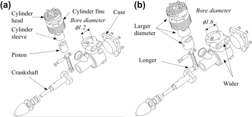
For example, the bore diameter of an engine case is defined as the design variable, as shown in Figure 3.20a. When the diameter is changed from 1.2 to 1.6 in., the engine case is regenerated first by properly updating its solid features that are affected by the change. As shown in Figure 3.20b, the engine case becomes wider and the distance between the two exhaust manifolds is larger, just to name a few. At the same time, the change propagates to other parts in the assembly, including the piston, piston pin, cylinder head, cylinder sleeve, cylinder fins, and crankshaft, as illustrated in Figure 3.20b. More important, the parts stay intact, maintaining adequate assembly mating constraints, and the change does not induce interference nor leave excessive gaps between parts. With such parametric models, design optimization can be carried out without the interruption of a failed model regenerating during the design iterations.
In addition to geometric dimensions, material parameters (e.g., modulus of elasticity) and physical parameters (e.g., spring constant) can also be included as design variables for design optimization. On the other hand, for design problems involving idealized structural models that are analyzed by using finite element analysis, such as a thin shell modeled in surface and beams as line models, thickness and cross-section properties (e.g., area or moment of inertia) defined at individual finite elements can be defined as design variables. Although these design variables are less intuitive physically, they are commonly employed for design optimization in FEA-based optimization tools, such as ANSYS. More about FEA-based optimization tools are discussed in Section 3.9.2.
3.8.2. Tool Integration for Design Optimization
Three major tools are critical for support of design optimization, modeling, analysis, and optimization. Modeling tool provides designers the capability of creating product design model, either part (in CAD or FEA tools) or assembly. Analysis tools support function evaluations, depending on the kinds of physical problems being solved. The physical problems can be single disciplinary, which involve a single engineering discipline, such as structural analysis with function evaluations for stress, displacement, buckling load factor, and so forth. On the other hand, the physical problems can be multidisciplinary, in which two or more engineering disciplines are involved, such as motion analysis of a mechanism (for reaction force calculation), structural analysis for load carrying components of the mechanism, machining simulation (for machining time calculation and manufacturing cost estimate), and so forth. Finally, optimization tools that offer desired optimization algorithms for searching for optimal design are essential. In many situations, gradient calculations (also called design sensitivity analysis) play an important role in design optimization. This is because, in general, gradient-based optimization techniques that require much less function evaluations compared to the non-gradient approaches are the only viable approach to support design problems involved large-scale physical models. Moreover, accurate gradient information facilitates the search for optimal solutions, and often requires fewer design iterations. More about gradient calculations are discussed in Chapter 4.
In the following, we present a case of tool integration for CAD-based mechanism optimization, in which kinematic and dynamic analysis is required for function evaluations. This integrated system has been applied to support the suspension design of a high-mobility multipurpose wheeled vehicle (HMMWV) (Chang 2013a).
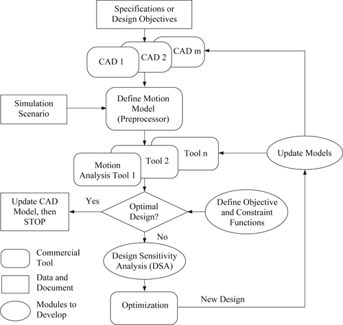
In this integrated system, commercial codes are first sought to support modeling, analysis, and optimization. In addition to the commercial codes, a number of software modules need to be implemented to support the tool integration, such as interface modules for data retrieval and model update modules for updating CAD and simulation models in accordance with design changes. The overall flowchart of the software system that supports CAD-based mechanism optimization is illustrated in Figure 3.21. The system consists of Pro/ENGINEER and SolidWorks for product model representation, Dynamic Analysis and Design System (DADS; Haug and Smith 1990) for kinematic and dynamic analysis of mechanical systems including ground vehicles, and Design Optimization Tool (DOT; www.vrand.com/dot.html) for a gradient-based design optimization. In this case, the overall finite difference method has been adopted to support gradient calculations.
In this system, engineers will create parts and assemblies of the product in a CAD tool. The solid model will be parameterized by properly generating part features and assembly constraints, as well as relating geometric dimensions to capture the design intents, as discussed in Section 3.8.1. Independent geometric dimensions of significant influence on the motion characteristics of the mechanical system are chosen as design variables. Consequently these variables help engineers achieve the design objectives more effectively.
The preprocessor supports design engineers in defining a complete motion model derived from the CAD solid model. Key steps include assigning a body local coordinate system (usually the default coordinate system in CAD), defining connections (or joints) between bodies, specifying initial conditions, and creating loads and drivers for dynamic and kinematic analyses. More about motion model creation and simulation can be found in Chang 2013a.
Design sensitivity analysis (DSA) calculates gradients of motion performance measures of the mechanical system with respect to dimension design variables in CAD. This is critical for optimization. The gradient information provides engineers with valuable information for making design decisions interactively. At the same time, it supports gradient-based optimization algorithms in searching for an optimal design. The gradient information and performance measure values are provided to the optimization algorithms in order to find improved designs during optimization iterations. In general, an analytical DSA method for gradient calculations is desirable, in which the derivative of a motion performance ψ with respect to CAD design variables x can be expressed as follows:
![]() (3.92)
(3.92)
where x = [d, c]T is the vector of design variables; d is the vector of dimension design variables captured in CAD solid models; c is a vector of physical parameters included in a load or a driver, such as the spring constant of a spring force created in the analysis model; m is the vector of mass property design variables, including mass center, total mass, and moment of inertia; and p is the vector of joint position design variables. In many situations, analytical methods for gradient calculations are not available; the overall finite difference method is an acceptable alternative, in which the derivative of a motion performance ψ with respect to CAD design variables x can be expressed as follows:
![]() (3.93)
(3.93)
where ψ(x) is a dynamic performance of the mechanical system at the current design, and ψ(x + Δxi) is the performance at the perturbed design with a design perturbation Δxi for the ith design variable. Note that the design perturbation Δxi is usually very small.
The motion model must be updated after a new design is determined in the optimization iterations. Mass properties and joint locations of the new design must be recalculated according to the new design variable values. The new properties and locations will replace the existing values in the input data file or binary database of the motion model for motion analysis in the next design iteration. Note that the definition of the motion model is assumed to be unchanged in design iterations; for example, no new body or joint can be added, driving conditions cannot be altered, and the same road condition must be kept during design iterations. Mass properties, joint locations, and physical parameters that define forces or torque (e.g., spring constant) are allowed to change during design iterations.
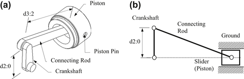
A simple slider crank example shown in Figure 3.22a is presented to demonstrate the feasibility of the integrated system. Schematically, the mechanism is a standard 4-bar linkage, as illustrated in Figure 3.22b. Moreover, geometric features in the crankshaft and connecting rod have been created with proper dimensions and references such that when their lengths are changed, the entire parts vary accordingly. At the assembly level, when either of the two length dimensions d2:0 or d3:2 is changed, the change is propagated to the affected parts. The remaining parts are kept unchanged, and the entire assembly is kept intact, as illustrated in Figure 3.23.
The CAD and motion models are created in SolidWorks and SolidWorks Motion, respectively. The mechanism is driven by a constant torque of 10 in-lb. applied to the crankshaft for 5 s. Note that friction is assumed to be nonexisting in any joint. The optimization problem is formulated as follows:
![]() (3.94a)
(3.94a)
![]() (3.94b)
(3.94b)
![]() (3.94c)
(3.94c)
![]() (3.94d)
(3.94d)
![]() (3.94e)
(3.94e)
![]() (3.94f)
(3.94f)
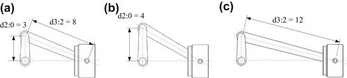
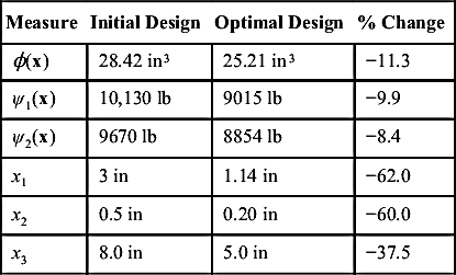
where the objective function ϕ(x) is the total volume of the mechanism; ψ1(x) and ψ2(x) are the maximum reaction forces in magnitude at the joints between crank and bearing, and between crank and rod, respectively, during a 5-s simulation period; and x1, x2, and x3 are design variables specifying the crankshaft length (d2:0), crankshaft width, and rod length (d3:2), respectively. At the initial design, we have x1 = 3 in, x2 = 0.5 in, and x3 = 8 in, as shown in Figure 3.24a. The maximum reaction forces are 10,130 and 9670 lb, respectively; therefore, the initial design is infeasible. The optimization took 15 iterations to converge using the modified feasible direction (MFD) algorithm (Vanderplaats 2005) in DOT. At the optimum, the overall volume of the mechanism is reduced by 11%, both performance constraints are satisfied, and two out of the three design variables reached their respective lower bounds, as listed in Table 3.1. The optimized mechanism is shown in Figure 3.24b. Note that all three design variables are reduced to achieve an optimal design because the design directions that minimize the total volume and reduce reaction forces between joints (due to mass inertia) are consistent.
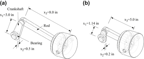
Table 3.1
Design Optimization of the Slider-Crank Mechanism (Chang and Joo 2006)
| Measure | Initial Design | Optimal Design | % Change |
| ϕ(x) | 28.42 in3 | 25.21 in3 | −11.3 |
| ψ1(x) | 10,130 lb | 9015 lb | −9.9 |
| ψ2(x) | 9670 lb | 8854 lb | −8.4 |
| x1 | 3 in | 1.14 in | −62.0 |
| x2 | 0.5 in | 0.20 in | −60.0 |
| x3 | 8.0 in | 5.0 in | −37.5 |
3.8.3. Interactive Design Process
For practical design problems, a true optimal is not necessarily sought. Instead, an improved design that eliminates known problems or deficiencies is often sufficient. Also, as mentioned earlier, function evaluations require substantial computation time for large-scale problems. Therefore, even using the gradient-based solution techniques, the computation may take too long to converge to an optimal solution.
In addition to batch-mode design optimization, an interactive approach that reduces number of function evaluations and design iterations is desired, especially for large-scale problems. In this subsection, we discuss one such approach called three-step design process, involving sensitivity display, what-if study, and trade-off analysis. The interactive design approach mainly supports the designer in better understanding the behavior of the design problem at the current design and suggests design changes that effectively improve the product performance in one or two design iterations.
3.8.3.1. Sensitivity display
The derivatives (or gradients) of functions with respect to design variables are called design sensitivity coefficients or gradients. These coefficients can be calculated, for example, using the overall finite difference method mentioned in Section 3.8.2. Once calculated, the coefficients can be shown in a matrix form, such as in a spreadsheet, as shown in Figure 3.25. Individual rows in the matrix display numerical numbers of gradients for a specific function (e.g., von Mises stress in Row 3 in Figure 3.25) with respect to all design variables; that is, ∂ψi/∂xj, j = 1, number of design variables (which is three in the matrix of Figure 3.25). Each row of the matrix shows the influence of design variables to the specific function (either objective or constraint). On the other hand, individual columns in the matrix display gradients of all functions with respect to a single design variable; that is, ∂ψi/∂xj, i = 1, number of functions. Each column shows the influence of the design variable to all functions.
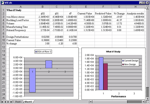
The design sensitivity matrix contains valuable information for the designer to understand structural behavior so as to make appropriate design changes. For example, if the von Mises stress is greater than the allowable stress, then the data in Row 3 show a plausible design direction that reduces the magnitude of the stress measure effectively. In the bar chart of the Row 3 data shown in the lower left of Figure 3.25, increasing the first design variable reduces stress significantly because the gradient is negative with a largest magnitude. On the other hand, decreasing the second design variable reduces the stress because the gradient of the design variable is positive. Changing the third design variable does not impact the stress because its gradient is very small. In fact, data in each row show the steepest ascent direction for the respective function (in increasing its function value). Reversing the direction gives the steepest descent direction for design improvement. By reviewing row or column data of the sensitivity matrix in bar charts, designers gain knowledge in the behavior of the design problem and possibly come up with a design that improves respective functions. Once a design change is determined, the designer can carry out what-if study that calculates the function values at the new design using first-order approximations without going over analyses for function evaluations.
3.8.3.2. What-if study
A what-if study, also called a parametric study, offers a quick way for the designer to find out “What will happen if I change a design variable this small amount?” In what-if study, the function values at the new design are approximated by the first-order Taylor's series expansion:
![]() (3.95)
(3.95)
where ψi is the ith function of the design problem, ∂ψi/∂xj is the design sensitivity coefficient of the ith function with respect to the jth design variable, and δxj is the design perturbation of the jth design variable. The what-if study gives quick first-order approximation for product performance measures at the perturbed design without going through a new analysis, for example, by using a finite element code.
In general, a design perturbation δx is provided by the designer, calculated along the steepest descent direction of a function with a given step size, or computed in the direction found by the trade-off determination to be discussed next, with a step size α; that is, δx = αn. The what-if study results and the current function values can be displayed in a spreadsheet or bar charts, such as that shown in Figure 3.25 (lower right). These kinds of displays allow the designer to instantly identify the predicted performance values at the perturbed design and compare them with those at the current design.
Once a better design is obtained from the what-if study (in approximation), the designer may commit to the changes by updating the CAD and analysis models, then carrying out analyses for the updated model to confirm that the design is indeed better. This completes one design iteration in an interactive fashion. Note that to ensure reasonably accurate function predictions using Eq. 3.95, the step size α must be small so that the perturbation  is, as a rule of thumb, less than 10% of the function value ψi(x).
3.8.3.3. Trade-off determination
In many situations, functions are in conflict due to a design change. A design may bring an infeasible design into a feasible region by reducing constraint violations; in the meantime, the same change could increase the objective function value that is undesirable. Therefore, very often in the design process, the designer must carry out design trade-offs between objective and constraint functions.
The design trade-off analysis method presented in this section assists the designer in finding the most appropriate design search direction of the optimization problem formulated in Eq. 3.3, using four possible options: (1) reduce cost (objective function value), (2) correct constraint neglecting cost, (3) correct constraint with a constant cost, and (4) correct constraint with a cost increment. As a general rule of thumb, the first algorithm, reduce cost, can be chosen when the design is feasible. When the current design is infeasible, among the other three algorithms, generally one may start with the third option, correct constraint with a constant cost. If the design remains infeasible, the fourth option, correct constraint with a cost increment of, say, 10%, may be chosen. If a feasible design is still not found, the second algorithm, correct constraint neglecting cost, can be selected. A QP subproblem, discussed in Section 3.6.4, is formulated to find the search direction numerically corresponding to the option selected.
The QP subproblem for the first option (cost reduction) can be formulated as
![]() (3.96a)
(3.96a)
![]() (3.96b)
(3.96b)
![]() (3.96c)
(3.96c)
For the second option (constraint correction neglecting cost), the QP subproblem is formulated as
![]() (3.97a)
(3.97a)
![]() (3.97b)
(3.97b)
![]() (3.97c)
(3.97c)
Note that Eq. 3.97 is similar to 3.96, except that the first term of the objective function in Eq. 3.96a is deleted in Eq. 3.97a because the cost (objective function) is neglected.
For the third option (constraint correction with a constant cost), the QP subproblem is the same as Eq. 3.97, with an additional constraint cTd ≤ 0 (implying no cost increment). For the last option (constraint correction with a specified cost), the QP subproblem is the same as Eq. 3.97, with an additional constraint cTd ≤ Δ, where Δ is the specified cost increment (implying the cost cannot increase more than Δ). The QP subproblems can be solved using a QP solver, such as MATLAB.
After a search direction d is found by solving the QP subproblem for the respective option, it is normalized to the vector n = d/||d||. Thereafter, a number of step sizes αi can be used to perturb the design. Objective and constraint function values, represented as ψi, at a perturbed design x + αin can be approximated by carrying out a what-if study. Once a satisfactory design is identified after trying out different step sizes in an approximation sense, the design model can be updated to the new design for the next design iteration.
A particular advantage of the interactive design approach is that the designer can choose proper option to perform design trade-offs and carry out what-if studies efficiently, instead of depending on design optimization algorithms to find a proper design by carrying out line searches using several function evaluations, which is expensive for large-scale problems. The result of the interactive design process can be a near-optimal design that is reliable. A case study is presented in Section 3.10.1 using a tracked-vehicle roadwheel example to further illustrate the interactive design process.
..................Content has been hidden....................
You can't read the all page of ebook, please click here login for view all page.