Perturbation of shape design variables results in the movement of the design boundary, as discussed in the previous section. Interior material points, or finite element nodes, in the structural domain must also move following certain rules. Among numerous approaches for domain velocity field computations, we briefly discuss two representative methods: the boundary displacement method and the isoparametric mapping method (Choi and Chang 1994).
4.5.4.3.1. Boundary displacement method
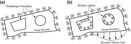
In the boundary displacement method, movements of nodal points at the design boundary are treated as the prescribed displacements. The domain velocity field that corresponds to the design perturbation can be obtained by solving an auxiliary elasticity problem with prescribed displacements specified at design boundary nodes as well as prescribed rollers at the nondesign boundary, as depicted in Figure 4.23. Note that rollers are added to constrain the nodal point movements at the nondesign boundary, as shown in Figure 4.23b, in accordance with the design intent.
FIGURE 4.23Illustration of the boundary displacement method for domain velocity field computation. (a) The original structure with boundary conditions. (b) The boundary velocity field added to the design boundary and additional rollers added to the nondesign boundary.
To form the auxiliary problem for the domain velocity computation, both the velocity field of the design boundary and the displacement constraints (e.g., rollers) that define nodal point movements on the nondesign boundary must be imposed to the finite element model. The discretized equilibrium equation of the auxiliary finite element model can be written as
KV=f
(4.262)
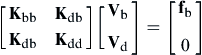
where K is the reduced stiffness matrix of the auxiliary structure (e.g., the structure shown in Figure 4.23b, which is different from that of the original structure (e.g., the one shown in Figure 4.23a. V is the design velocity vector and f is the unknown vector of boundary forces, which produce the prescribed boundary velocity at both the design and nondesign boundary. In a partitioned form, Eq. 4.262 can be written as
[KbbKdbKdbKdd][VbVd]=[fb0]
(4.263)
where Vb is the prescribed velocity of nodes on the boundary, Vd is the nodal velocity vector in the interior domain (domain velocity), and fb is the unknown boundary force that acts on the structural boundary. Equation 4.263 can be rearranged as
KddVd=−KdbVb
(4.264)
This defines a linear relationship between the boundary and domain velocity fields.
The boundary displacement method is independent of the way in which the boundary velocity field is computed. The same finite element code used for analysis can be used to compute the displacement field of the auxiliary model; yielding a domain velocity field that naturally satisfies the linearity requirement (because the finite element matrix equations are a system of linear equations). An important characteristic of the elasticity problem is that the solution trajectory tends to maintain orthogonality. As a result, the updated mesh obtained using the velocity field, as stated in Eq. 4.242, tends to be more regular (see Figure 4.26 as an example).
One drawback of the boundary displacement method is that finite element matrix equations must be formulated and solved to generate the velocity field for each shape design variable. For this, the reduced stiffness matrix of the auxiliary finite element model must be formed and decomposed for each design variable. Once the design velocity field is calculated, it can be used throughout the design iterations.
4.5.4.3.2. Isoparametric mapping method
The isoparametric mapping method is far more efficient than the boundary displacement method because the former needs only a few matrix multiplications. However, the essence of the isoparametric method is the availability of a mapping function N that maps nodal points from parametric coordinates (u,w) of the geometric model to Cartesian coordinates (x,y,z), as illustrated in Figure 4.24.
In Figure 4.24, the structural domain is meshed into 5 × 3 finite elements. If the nodes are evenly distributed in the (u,w) space, the parametric coordinates of individual nodes are readily available. For example, the parametric coordinates of node 8 are (u8,w8) = (0.2, 0.667). To simplify the mathematical expressions in our discussion, we assume a 2-D planar structure for discussing the parametric mapping method.
FIGURE 4.24Concept of isoparametric mapping.
Finding an appropriate mapping function N for accurate velocity field computation is difficult when the geometric shape of the structure is complicated. However, for a simple geometric model or a smaller subdomain of the structure, for which an accurate mapping function N can be found, the isoparametric mapping method is attractive. For such a model or subdomain that can be modeled by a single geometric entity, velocity fields can be computed using the isoparametric mapping method.
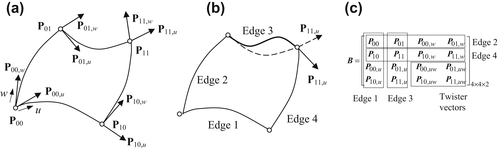
Geometric modeling software, such as MSC/PATRAN and HyperMesh, employs a standard patch to represent geometric surfaces. For example, in PATRAN, a surface patch is modeled in Coons patch (Mortenson 2006). A Coons patch, as shown in Figure 4.25a, is a bicubic parametric surface in terms of parametric coordinates u and w, where u and w ∊ [0,1]. Obviously, one single patch is not able to represent a complicate geometric entity. Therefore, a 2-D structural domain is often decomposed into several smaller patches in the modeling process.
FIGURE 4.25A bicubic parametric patch. (a) Corner points and tangent vectors. (b) Adjusting tangent vector P11,u. (c) Data formulated in a 4 × 4 × 2 B-matrix that defines the patch.
FIGURE 4.26The two-dimensional fillet example modeled in two patches. (a) Original mesh. (b) Remesh using the boundary displacement method. (c) Remesh the using mapping method (Choi and Chang 1994).
The edges of a Coons patch are cubic curves in u and w, respectively. The shape of the cubic curve can be controlled by adjusting tangent vectors in both direction and magnitude. For example, changing the direction of the tangent vector P11,u will alter the geometry of edge 3 and, therefore, the geometry of the patch, as illustrated in Figure 4.25b. A mesh of quad-elements can be generated by specifying the number of elements along the u- and w-parametric directions, such as the mesh shown in Figure 4.24, in which the number of elements along the u- and w-parametric directions are 5 and 3, respectively.
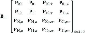
The data representation of a Coons patch is in a so-called B-matrix, as shown in Figure 4.25c, defined as
where P00 = S(0,0), P01 = S(0,1), P10 = S(1,0), and P11 = S(1,1) are the four corner points; P00,u = ∂S/∂u|u=w=0, P01,u, P10,u, and P11,u are the tangent vectors in the u-direction at the four corner points; P00,w = ∂S/∂w|u=w=0, P01,w, P10,w, and P11,w are the tangent vectors in the w-direction at the four corner points; and P00,uw = ∂2S/∂u∂w|u=w=0, P01,uw, P10,uw, and P11,uw are the twister vectors at the four corner points. Note that a twister vector represents changes of tangent vector in the u (or w)-direction at a corner point along a boundary curve in the w (or u)-direction. For example, P10,uw = ∂/∂w(∂S/∂u)|u=1, w=0 = ∂P10,u/∂w is the derivative of the tangent vector along the u-direction at P10 with respect to w. The same twister vector can also be interpreted as P10,uw = ∂/∂u(∂S/∂w)|u=1, w=0 = ∂P10,w/∂u, which is the derivative of the tangent vector along the w-direction at P10 with respect to u. Note that for a planar patch, all twister vectors vanish. Also, the first two columns of the B matrix are boundary edges 1 and 3, respectively; and rows 1 and 2 are boundary edges 2 and 4, respectively.
Recall that the mathematical expression (algebraic format) for a bicubic parametric surface was given in Eq. 4.226. Similar to a Bézier surface, a Coons patch can also be written in a form like that of Eq. 4.227:
Here, H = [P0, P1, P0,u, P1,u]T, in which P0 and P1 are the end points and P0,u and P1,u are tangent vectors at the end points. Entries in the matrix H can be used for shape design variables, depending on which boundary edge the curve represents. Any change in H alters the shape of the Coons patch:
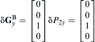
For example, if the y-component of the tangent vector along the u-direction at (u,w) = (1,1)—that is, P11y,u—is varied by δP11y,u = 1, then δB is
δBy=[0000000000000100]4×4
(4.271)
In this case, δBx(u,w) = 0 because no change occurs in the x-direction. The domain velocity can be calculated by plugging the (u,w) of the node into Eq. 4.269. Note that in Eq. 4.270, we set the variation of the twister vectors to zero for planar structures.
EXAMPLE 4.22
Assume that δP11y,u = 1. Calculate the velocity for node 8 (n8) shown in Figure 4.24, where (u8,w8) = (0.2, 0.667).
Solutions
Using Eq. 4.269 with δBy shown in Eq. 4.271, we have
If the boundary curve is not parameterized using a Hermit cubic curve, the change in the curve must be transformed to a Hermit cubic form and then the perturbed B matrix δB is created accordingly. For example, a cubic curve defined in Eq. 4.216 can be written as Bézier curve or a Hermit cubic curve, as follows:
P(u)=U(u)A=UNBGB=UNCH
(4.272)
Here, GB contains the four control points of the cubic Bézier curve, and H was defined in Eq. 4.268, consisting of the end points and tangent vectors of a Hermit cubic curve. Therefore, control point vector of a Bézier curve can be transformed into an H vector of a Hermit cubic curve as
H=(NC)−1NBGB
(4.273)
Then, the changes in a Bézier curve can be transformed into a change in the Hermit cubic curve:
δH=(NC)−1NBδGB
(4.274)
EXAMPLE 4.23
Assume that the design boundary of the patch that contains nodes n1 to n6 shown in Figure 4.24 is parameterized by a Bézier curve identical to that of Example 4.18. As stated in Example 4.18, the design change is δb = δP2y = 1; that is, the design variable is the y-direction movement of control point P2. Note that the design boundary is edge 3 of a Coons patch shown in Figure 4.25b. Calculate the velocity for node 8 inside the patch.
Solutions
From Example 4.18, the ∂GBy of the Bézier curve is
Using Eq. 4.269 with the second column of δBy in Eq. 4.271 (with edge 3 as the design boundary in this case) replaced by the vector δHy in Eq. 4.276, we have
Hence, the domain velocity at node 8 is obtained as V8 = [0,−0.2846].
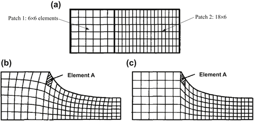
As mentioned before, the isoparametric mapping method is much more efficient than the boundary displacement method; however, the velocity field obtained using the boundary displacement method tends to keep the finite element mesh more regular because tracing of the solution to an elastic problem, governed by partial differential equations, is more orthogonal. Figure 4.26a shows a 2-D fillet example, in which the finite element mesh updated using the velocity obtained from the boundary displacement method (Figure 4.26b) is of better quality than those updated using isoparametric mapping method. Figure 4.26c shows that, using isoparametric mapping, the finite element mesh could be severely distorted after a large design change (e.g., element A).
4.5.5. Shape Sensitivity Analysis Using Finite Difference or Semianalytical Method
As with the sensitivity analysis for sizing or material design variables, shape DSA can be carried out using the overall finite difference or semianalytical method, in which a design variable is perturbed and a finite element model is regenerated with the design change. These methods are general and widely employed in support of gradient-based optimization, despite the drawbacks pointed out previously.
For shape sensitivity analysis using the finite difference method or semianalytical method, it is desirable to update the finite element model (using Eq. 4.242) at the perturbed design using a velocity field obtained from the methods discussed above. In the overall finite difference method, an FEA is carried out for the FE model at the perturbed design, then the sensitivity coefficient is approximated using Eq. 4.35. In the semianalytical method, the stiffness matrix and load vector of the perturbed design must be generated, and Eq. 4.41 is followed to calculate the sensitivity coefficients.
In many situations, the design velocity field may not be readily available. Overall, the finite difference method is widely implemented for shape sensitivity analysis using CAD software equipped with a mesh generator and FEA solver, such as SolidWorks Simulation. A new dimension value with a design perturbation can be entered in CAD and the solid model can be rebuilt and remeshed. Thereafter, an FEA model for the perturbed design can be created (usually meshed by an automatic mesh generator), and an FEA can be carried out. The results obtained from FEA of the current and perturbed designs can then be used for sensitivity calculations using Eq. 4.35.
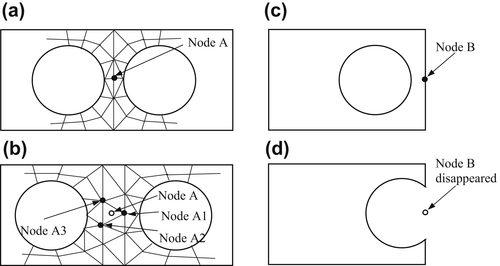
Although the approach is easy to implement, it has two potential pitfalls in addition to the problems of step size determination and computation efficiency, as discussed in Section 4.3. For shape design, the added pitfalls are altering topology of finite element mesh or geometric features at the perturbed design, as illustrated in Figure 4.27.
The pitfalls affect local performance measures, such as the stress measure defined at node A shown in Figure 4.27a. We assume a design change pulls the holes further apart. As a result, mesh is regenerated due to a design perturbation, as shown in Figure 4.27b. Due to the change in mesh topology, there is no clear trace in locating node A in the perturbed design: Is it at node A1, A2, or A3 that the stress performance is to be measured for sensitivity calculation using finite difference method? Another such example is the disappearing of nodes where performance measures are defined. As shown in Figure 4.27c, a performance measure, such as displacement, is defined at node B. Due to a design perturbation, the hole is moved to the right, such that it intersects the right edge of the rectangular structural boundary. As a result, part of the right edge disappears, as well as node B. Such a topology change in geometric features cause problems in calculating shape sensitivity coefficients using finite difference method with CAD software.
4.5.6. Material Derivatives
Besides finite difference and semianalytical methods, the continuum approach offers options for shape sensitivity analysis with a rigorous mathematical basis and better computational efficiency. Moreover, no step size is required for design perturbation, such as in the finite difference and semianalytical methods.
The key theory in continuum approach for shape sensitivity analysis is the material derivative. In general, the material derivative describes the time rate of change of a physical quantity, such as heat or momentum, for a material element subjected to a space- and time-dependent velocity field. For structural shape design, time is replaced by design change, and the time rate of change of a physical quantity becomes the rate of a performance measure change with respect to design (i.e., gradient or sensitivity coefficient).
Recall the energy bilinear form and load linear form discussed in Section 4.4.1, which governs the behavior of the structure under static load:
aΩ(z,¯z)=ℓΩ(¯z),∀¯z∈S
(4.277)
FIGURE 4.27Pitfalls in shape sensitivity analysis using finite difference or semianalytical methods with the mesh generator in CAD software: (a) mesh of current design, (b) mesh topology altered after design change, (c) Node B at the right edge of the current design, and (d) topology of geometric features altered eliminating Node B.
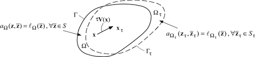
Note that the subscript Ω is added to the energy and load forms in Eq. 4.277 to emphasize their dependence on the structural domain Ω, which varies. In Eq. 4.277, z is the solution, or displacement, of the governing equation of the structure at the current design, in which the structural domain is Ω, as illustrated in Figure 4.28.
Let zτ(xτ) be the solution of the same governing equation but at a perturbed domain Ωτ due to a design change:
aΩτ(zτ,¯zτ)=ℓΩτ(¯z),∀¯zτ∈Sτ
(4.278)
Here, the energy bilinear form and load linear form are formulated at the new structural domain Ωτ, and Sτ is the space of kinematically admissible virtual displacement at the new design. Note that, in general, S = Sτ because the essential boundary conditions do not change with design and the smoothness of the solution function is not affected by the shape change. Again, τ is a scalar parameter that defines a shape change. In a material derivative for a physical problem, τ plays the role of time.
FIGURE 4.28Illustration of material derivative concept.
It is important to note that the displacement zτ(xτ) at the new design is a new function zτ and measured at the new location xτ, which is determined by the design velocity field V, as discussed in Section 4.5.4. As discussed before, for a linear design velocity field, xτ is determined by
xτ=x+τV
(4.279)
Expanding zτ(xτ) using Taylor's series, we have
zτ(xτ)=zτ(x+τV)≈zτ(x)+∇[zTτ(x)](τV)+…
(4.280)
Here, the gradient operator is employed—that is, ∇ = [∂/∂x1, ∂/∂x2, ∂/∂x3]T, which is a 3 × 1 vector for three-dimensional structures. The material derivative of a function, such as the displacement, is defined as
˙z(x)≡ⅆzτ(xτ)ⅆτ|τ=0=ⅆzτ(x+τV)dτ|τ=0
(4.281)
in which the dot on top of the function z denotes the material derivative on z. Equation 4.281 can be rewritten in a limiting form as
The first term on the right-hand side of Eq. 4.282 defines the change of the same function zτ evaluated at different locations (xτ and x respectively). This can be further derived using the expansion shown in Eq. 4.280 as
The second term on the right-hand side of Eq. 4.282 defines the change due to different functions (zτ and z) evaluated at the same location x, which is nothing but the variation of z from its definition discussed in Section 4.4.2:
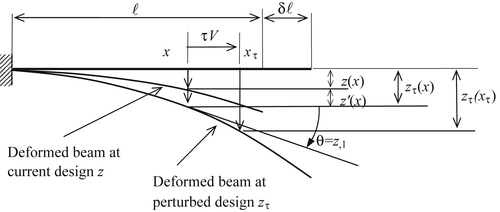
The physical meaning of Eq. 4.285 can be illustrated using a cantilever beam example shown in Figure 4.29, in which z = z3 = z (subscript 3 is omitted for simplicity), x = x1 = x (subscript 1 is omitted), and V = V1 = V (subscript 1 is omitted). Hence, Eq. 4.285 is reduced to
˙z(x)=z′+z,1V
(4.286)
in which V is the design velocity that determines the material point movement due the beam length change. As shown in Figure 4.29, the difference between z(x) and zτ(xτ) consists of two parts, z′(x) ≈ zτ(x) −z(x) and θ·(xτ−x) = z,1τV.
FIGURE 4.29Deformed cantilever beam at current and perturbed designs due to a length change.
Recall that the FEA solution for the cantilever beam with an evenly distributed load shown in Figure 4.13 is obtained in Eq. 4.200 as
z3(x)=qℓ24EI(5x2ℓ−2x3)
(4.287)
In the next example, we use this solution to further illustrate the concept of material derivatives for the cantilever beam example shown in Figure 4.13.
EXAMPLE 4.24
Calculate ˙z, z′, and z,1V at x=ℓ for the cantilever beam shown in Figure 4.13, using the finite element solution of Eq. 4.200.
Solutions
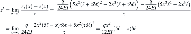
We first evaluate z′ from the definition stated in Eq. 4.284. The displacement at the perturbed design due to the change δℓ in the length of beam can be found as
For simplicity in shape sensitivity analysis, we set δℓ=1. Note that Eq. 4.289 is nothing but ∂z3(x)∂ℓ shown in Eq. 4.208. Evaluating Eq. 4.289 at x=ℓ, we have
z′=qℓ33EI
(4.290)
which is identical to Eq. 4.209. Now, we take the derivative of Eq. 4.200 with respect to x:
which is ∂zℓ3∂ℓ=qℓ32EI, as obtained in Eq. 4.202 (and Eq. 4.207).
As demonstrated in Example 4.24, for the cantilever beam example, the sensitivity coefficient obtained using the discrete approach discussed at the beginning of this section is the same as the result of material derivative, in which the measurement point is assumed to be moving with the design. On the other hand, the result obtained in Eq. 4.209 is nothing but z′, in which the measurement point is assumed to be stationary. As discussed, the movement of the material point or the measurement point is determined by the design velocity field. At the boundary, the velocity field is δℓ. How do the interior points move due to the design change δℓ? How does the domain velocity field affect the shape sensitivity coefficient?
Now, we discuss further on the design velocity field. At the tip, the boundary velocity is defined as δℓ. The interior or domain velocity can be defined in different ways, depending on the design intent. For example, let us consider two design velocity fields VA and VB, shown in Figures 4.30a and 4.30b, respectively. VA is a linear function, and VB is a quadratic function. Both assume a length change at the right end by δℓ. Mathematically, they are defined as
VA=xℓδℓ
(4.294)
VB=(xℓ)2δℓ
(4.295)
No matter how the velocity field is defined, the z′ term is unchanged because the functions zτ and z are evaluated at the same point. The same is true for z,1. The only term that is affected is the velocity field V in the second term of Eq. 4.287. We assume the displacement is measured at midpoint x=ℓ/2, the design velocities at the midpoint are δℓ/2 and δℓ/4, respectively, using VA and VB. Hence, the material derivatives of the displacement at the midpoint become
FIGURE 4.30Midpoint movement with design change δℓ. (a) δℓ/2: linear velocity. (b) αδℓ≠δℓ/2: other than linear velocity. (c) δℓ: beam length change is zero.
in which ˙zAℓ/2 predicts the displacement at the midpoint of the beam if the movement of the displacement measurement point is determined by velocity field VA when a beam length is changed by δℓ. Similarly, ˙zBℓ/2 predicts the displacement at the midpoint of the beam if the movement of the displacement measurement point is determined by velocity field VB. Therefore, in general, domain velocity is not unique, as long as it satisfies the requirements discussed in Section 4.5.4 and adequately captures the design intent.
We now take a look at a design velocity field VC shown in Figure 4.30c, which is defined as a quadratic function with zero at both ends and maximum at the midpoint. Mathematically, VC is defined as
VC=4xℓ2(ℓ−x)δℓ
(4.298)
In this case, the shape sensitivity coefficient at the tip is zero because V = 0 at x = l. However, at the midpoint, the sensitivity is not zero; instead
˙zCℓ/2=z′+z,1V=0+7qℓ348EI(δℓ)=7qℓ348EIδℓ
(4.299)
Here, z′ = 0 because the displacement function is unchanged (length stays constant). The second term of Eq. 4.299 is nonzero, which characterizes the change of displacement due to the change of the measurement point.
With a basic understanding of the concept of shape design, we move on to introduce the shape sensitivity analysis method based on the continuum approach. To simplify the mathematical derivations, we focus only on the beam example.
4.5.7. Shape Sensitivity Analysis Using the Continuum Approach
We start by stating one of the major material derivative equations that are essential for the continuum approach. Readers are referred to Choi and Kim (2006a) for details and mathematical proof of the equation.
For an integral function defined as
Φ=∫Ωτfτ(xτ)Ωτ
(4.300)
in which f is a scalar function, the material derivative of Φ is given as
˙Φ=(∫Ωτf(xτ)ċΩτ)=∫Ω(f′(x)+div(fV))Ω
(4.301)
in which the divergence is defined as div(fV) = (fV),1 + (fV),2 + (fV),3 for 3-D structures.
This equation is applied to the energy bilinear form and load linear form of Eq. 4.277. We rewrite the energy bilinear form as
aΩτ(zτ,ˉzτ)=∫Ωτc(zτ,ˉzτ)Ωτ
(4.302)
For a beam structure, c(z,ˉz)=EIz3,11ˉz3,11. The material derivative of aΩτ(zτ,¯zτ) can be written using Eq. 4.301:
in which we assume f′ = 0. Hence, equating ·[aΩτ(zτ,¯zτ)] and ·[ℓΩτ(¯zτ)], we have
aΩ(˙z,¯z)=−a′V(z,¯z)+ℓ′V(¯z),∀¯z∈S
(4.307)
Similar to sizing sensitivity analysis, in implementation, the right-hand side of Eq. 4.307 is calculated as a fictitious load, which is employed to solve for ˙z. Equation 4.307 represents the direct differentiation method of the continuum approach. For the adjoint variable method of the continuum approach, readers are referred to Choi and Kim (2006a).
4.5.7.1. Shape sensitivity analysis for a cantilever beam
For one-dimensional beam bending problems, we have c(z,¯z)=EIz3,11ˉz3,11, z = z3, VTn = V, ∇z = z3,1, and div f = f,1. Hence, from Eqs 4.304, 4.305, and 4.306, we have
Using finite element shape functions, such as those shown in Eq. 4.143, to discretize the sensitivity equation (Eq. 4.311), we have on the left-hand side
∫ℓ0EI˙z3,11ˉz3,11ⅆx=¯ZTgKg˙Zg
(4.312)
where
˙Zg=[˙z3i˙θi˙z3j˙θj]T
(4.313)
The right-hand side of Eq. 4.311 can be computed as ¯ZTFficg, in which Fficg is the global fictitious load vector. By imposing the boundary conditions and removing the virtual displacement ¯Z from both sides, we have
K˙Z=Ffic
(4.314)
which can be solved using the same decomposed stiffness matrix K as the original structure considering the fictitious load Ffic as additional load cases. Equation 4.311 represents the direct differentiation method of the continuum-discrete approach for shape sensitivity analysis. We illustrate a few more details in the following example.
EXAMPLE 4.25
Calculate shape sensitivity for the cantilever beam shown in Figure 4.13, assuming a linear design velocity of Eq. 4.294—that is, V=VA=xℓ (set δℓ=1)—using the continuum-discrete method.
Solutions
We first rewrite Eq. 4.311 for the cantilever beam with f = q (hence f,1 = q,1 = 0) and a linear velocity field (hence V,11 = 0) as
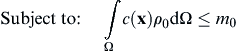
Sizing optimization varies the sizes of the structural elements, such as the diameter of a bar or beam, as shown in Figure 4.31a, or the thickness of a sheet metal. In sizing optimization, the shape of the structure is known and unchanged. For shape optimization, the topology of geometric features in the structure, such as the number of holes, is known. The optimal shape is confined to the topology of the initial structural geometry, as illustrated in Figure 4.31b. No additional holes can be created during the shape optimization process. For both sizing and shape optimization, the topology of the structural geometry is unchanged in the design process.
Another important type of optimization problem is topology optimization, which solves the basic engineering problem of distributing a prescribed amount of material in a design space. Topology optimization is sometimes referred to as layout optimization. In general, the goal of topology optimization is to find the best use of material for a structural body that is subject to either a single load or multiple load distributions. The best use of material in the case of topology optimization represents a maximum stiffness (or minimum compliance), maximum buckling load, or maximum first vibration frequency design. With topology optimization, the resulting shape or topology is not known; the number of holes, structural members (for frame structures), etc. are not decided upon, as illustrated in Figure 4.31c.
In topology optimization, we start from a given design domain and proceed to find the optimum distribution of material and voids. In general, a design domain is discretized by using the FEM into discrete mesh. Individual finite elements in the discretized design domain are then evaluated to determine if they are staying or removed from the structure using optimization methods. This results in a so-called 0–1 problem—the elements either exist or do not.
The two main solution strategies for solving the topology optimization problem are the density method and the homogenization method. In this section, we briefly discuss the density method. Those interested in learning the homogenization method are referred to Bendsøe and Sigmund (2003).
4.6.1. Basic Concept and Problem Formulation
In general, the objective of a topology optimization problem is either to minimize the compliance, which is equivalent to maximizing the stiffness, maximize the lowest frequency, or maximize the lowest buckling load. A volume constraint is imposed to limit material usage. The optimization problem can be formulated as
Minimize:ϕ(c(x))
(4.323a)
Subjectto:∫Ωc(x)ρ0ⅆΩ≤m0
(4.323b)
ψi−ψui≤0,i=1,m
(4.323c)
0≤c(x)≤1
(4.323d)
where ϕ is a structural performance measure to be minimized (or maximized), such as compliance; ψi is ith structural performance constraint, such as displacement; m is the total number of constraints; Ω is the structural domain; m0 is the mass limit; c(x) is the design variable; and ρ0 is material mass density. In implementation, the design variable c(x) is assigned to individual finite elements; therefore, c(x) = ci, i = 1, NE (number of elements). In each element, the density becomes ρi = ciρ0, and Eq. 4.323b becomes
∫Ωc(x)ρ0ⅆΩ=∑NEi=1ciρ0Vi≤m0
(4.324)
where Vi is the volume (or area for planar problems) of the ith finite element. Also, Eq. 4.323d becomes
0≤ci≤1,i=1,NE
(4.325)
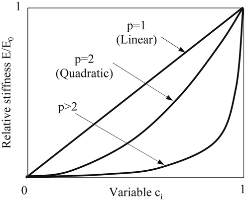
It is desired that the solution of topology optimization only consists of solid or empty elements—that is, ci = 0 or 1. One popular method to suppress or penalize intermediate densities is by letting the stiffness of the material be expressed as
E=cpiE0,i=1,NE
(4.326)
where E0 is the modulus of elasticity of the material and p is a penalization factor that is greater than zero, typically 2 to 5 in implementation. For p > 1, local stiffness for values of ci < 1 is lowered, as illustrated in Figure 4.32, thus making it “uneconomical” to have intermediate densities in the optimal design. In the literature, the density method together with this penalization is often called the SIMP (solid isotropic microstructures with penalization) method (Rozvany 2000).
Although the density method is straightforward to implement for topology optimization, one must be aware of numerical instabilities. These can manifest as checkerboard, mesh dependence, and local minimum. More detailed discussion and remedies to treat these instabilities can be found in Sigmund and Petersson (1998).
Topology optimization often converges to a design that contains a checkerboard pattern—that is, the alternately solid and void elements, as shown in Figure 4.33b. This is a typical result in topology optimization using finite element methods.
FIGURE 4.32Relative stiffness as a function of variable ci with different penalization factors p (Eschenauer and Olhoff 2001).
FIGURE 4.33Numerical instabilities in topology optimization. (a) Design problem. (b) Example of checkerboards. (c) Solution for 600-element discretization. (d) Solution for 5400-element discretization (Sigmund and Petersson 1998).
The quality of topology optimization result is dependent on the discretization of the finite element model, the so-called mesh-dependence problem. Figure 4.33c shows the topology optimization result for the discretization using 600 elements, and Figure 4.33d shows the result using 5400 elements for the same physical problem. The result in Figure 4.33d is much more detailed than that in Figure 4.33c; however, the two topologies are different in nature.
Different solutions to the same discretized problem are observed when choosing different parameters, such as finite element type (triangular vs quadratic elements), optimization algorithms, convergence criteria, and so forth. These numerical instabilities are all related to whether the continuous constrained optimization problems are well posed or not—that is, whether they have a solution or not.
4.6.2. Two-Dimensional Cantilever Beam Example
A cantilever beam with a fixed left end and a vertical load applied at the midpoint of the free end, as shown in Figure 4.34a, is used to illustrate the density method for topology optimization. The material properties are modulus of elasticity E = 2.07 × 10⁵ psi and Poisson's ratio ν = 0.3.
The finite element model contains 32 × 20 mesh with four-node quad elements. There are 640 elements in the model and the density of each element is selected as the design variable. The design problem is to minimize the compliance with the area constraint of 25% imposed on the domain. Figure 4.34b shows the material distribution using the modified feasible direction after 10 iterations. Figure 4.34c shows the material distribution using the sequential linear programming after 36 iterations. Figure 4.34d shows the material distribution using the sequential quadratic programming after 28 iterations. They converge to slightly different topologies.

 (4.263)
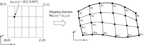
 (4.265)
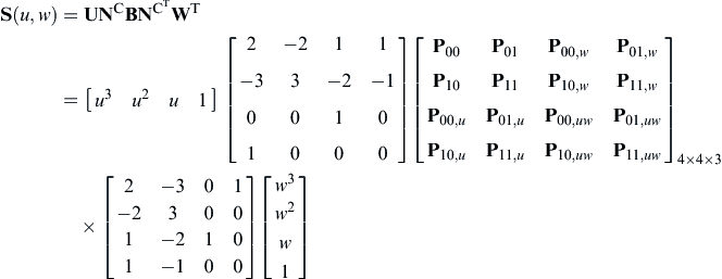 (4.266)
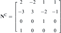 (4.267)
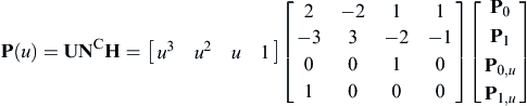 (4.268)
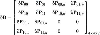 (4.270)
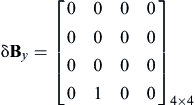 (4.271)
 (4.275)
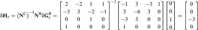 (4.276)
 (4.289)
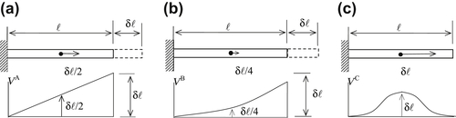
 . (a) δℓ/2
 : linear velocity. (b) αδℓ≠δℓ/2
 : other than linear velocity. (c) δℓ
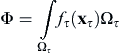 (4.300)
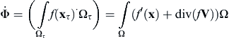 (4.301)
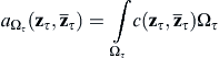 (4.302)
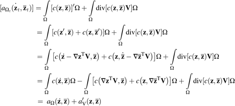 (4.303)
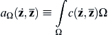 (4.304)
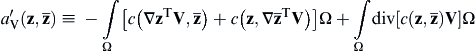 (4.305)
 (4.306)
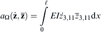 (4.308)
 (4.309)
 (4.310)
 (4.311)
 (4.312)
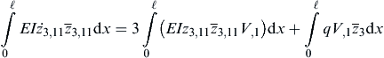 (4.315)
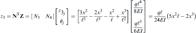 (4.316)
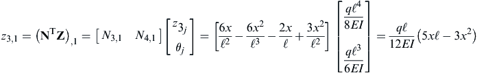 (4.317)
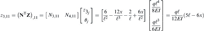 (4.318)
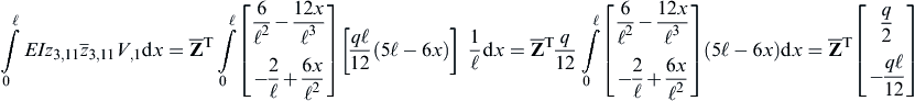 (4.319)
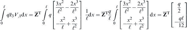 (4.320)
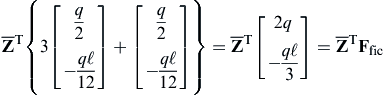 (4.321)
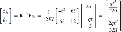 (4.322)
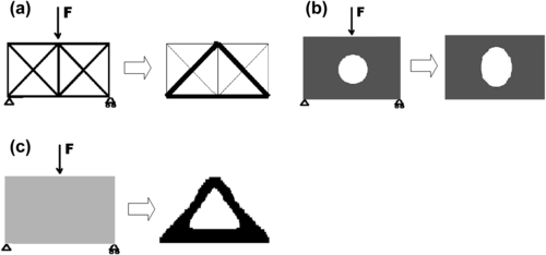
 (4.323b)
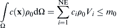 (4.324)