Search in book...
Toggle Font Controls
Create new playlist

Name your new playlist

Playlist description (optional)
Sign In

Email address

Password

Forgot Password?

or

Continue with Facebook

Continue with Google
Sign Up

Full Name

Email address

Confirm Email Address

Password

or

Continue with Facebook

Continue with Google

Project P5

Design with Pro/ENGINEER

Abstract

In Project P5, we introduce Pro/ENGINEER design optimization capabilities as well as conducting interactive design using the suite of Pro/ENGINEER CAD/CAE/CAM capabilities for a multidisciplinary design problem. We include an optimization design study for a cantilever beam as a single-objective optimization of single engineering discipline, including only structural performance measures. Then we present a single-piston engine example to illustrate the interactive design process discussed in Chapter 3 involving multiple engineering disciplines. For those who are not familiar with Pro/ENGINEER and embedded CAE/CAM modules, we encourage you to go over Projects P1 to P4 of the book series before moving forward with this tutorial project. Without going over these prior projects, you may get lost very quickly. Example models of the current project are available for download at the book’s companion website.

Keywords

Multidisciplinary optimization; design optimization; sensitivity analysis; what-if study

Design optimization was discussed in Chapters 3 and 5 for single-objective and multiobjective problems, respectively. In these chapters, both theoretical and practical aspects of the topics are discussed. With a basic understanding of concept, theories, and solution techniques of design optimization, we are ready to go over a few tutorial lessons on design optimization using the capabilities offered by commercial tools, such as Pro/ENGINEER.

In Project P5, we introduce Pro/ENGINEER design optimization capabilities as well as conduct interactive design using the suite of Pro/ENGINEER computer-aided design (CAD), engineering (CAE), and manufacturing (CAM) capabilities for a multidisciplinary design problem. We include an optimization design study for a cantilever beam as a single-objective optimization of single engineering discipline, including only structural performance measures. Then, we present a single-piston engine example to illustrate the interactive design process discussed in Chapter 3 involving multiple engineering disciplines. For those who are not familiar with Pro/ENGINEER and embedded CAE/CAM modules, we encourage you to go over Projects P1–P4 of the book series before moving forward with this tutorial project. Without going over these prior projects, you may get lost very quickly. Example models of the current project are available for download at the book's companion Web site.

Overall, the objective of this project is to enable readers to use Pro/ENGINEER for batch-mode design optimization and interactive design. The use of the capability for design optimization should be straightforward. Readers who are interested in learning more about the batch-mode optimization in Pro/ENGINEER may review a few more examples offered as YouTube videos, such as those listed below, subject to their availability:

• Pro/ENGINEER (Pro/E) Mechanica tutorial—Introduction to Optimization Design Study by eeprogrammer.com (www.youtube.com/watch?v=LrvvtKvse_A)

• Optimization Study in Wildfire 4.0 (www.youtube.com/watch?v=DzDlty6Vs9A)

Note that the lessons included in this current project were developed using Pro/ENGINEER Wildfire 5.0 M040. If you are using a different version of Pro/ENGINEER, you may see slightly different menu options or dialog boxes.

P5.1. Introduction to Design Optimization in Pro/ENGINEER

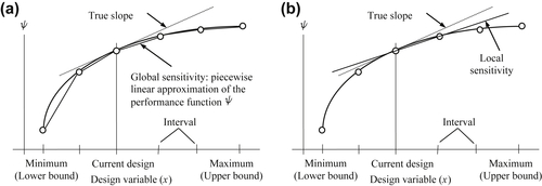
There are two main design study capabilities offered by Pro/ENGINEER—or more specifically, Pro/MECHANICA Structure (or Mechanica), which is a CAE module embedded in Pro/ENGINEER for support of finite element analysis (FEA) and design studies. These two design study capabilities are sensitivity and optimization. Sensitivity includes global and local sensitivity studies. A global sensitivity study calculates the changes in product performance measures when a design variable (or a combined change with more than one design variables) is varied over a prescribed range. Mechanica does this by calculating performance measure values at numerous designs in the design variable range(s). Design variables are perturbed a number of times (default is 10 in Mechanica) with a uniform design perturbation (or design interval). Mechanica automatically changes the solid model (provided that it is fully parameterized), updates finite element mesh, and analyzes the finite element model for each design change. This computation is usually very expensive (i.e., time-consuming) for large-scale models. Results of the global sensitivity study can be shown in a graph of a measure versus a design variable, essentially a piecewise linear approximation of the performance function ψ, as illustrated in Figure P5.1a.

A local sensitivity study calculates the gradient (slope) of a product performance measure with respect to a design variable. Mechanica calculates the slope of the performance curve ψ(x) between two sample points (usually, one of them is the current design). The local sensitivity is computed using the finite difference method:

$\frac{\partial ψ}{\partial x} \approx \frac{ψ (x + Δ x) - ψ (x)}{Δ x}$ $\frac{\partial ψ}{\partial x} \approx \frac{ψ (x + Δ x) - ψ (x)}{Δ x}$

(P5.1)

As discussed in Chapter 3, a sensitivity study using the finite difference method could be inaccurate. Accuracy is largely dependent on size of the perturbation Δx. Note that Mechanica determines the design perturbation Δx internally.

FIGURE P5.1 Sensitivity design studies: (a) global sensitivity and (b) local sensitivity.

An optimization design study, on the other hand, allows users to conduct a batch-mode optimization following gradient-based optimization approach, as discussed in Chapter 3. In this project, we focus on the optimization design study.

We use a cantilever beam example for illustration of the optimization capability (batch mode) in Section P5.2. The beam example is a single-objective optimization problem of single discipline, only involving structural performance measures. In addition, we use the single-piston engine example in Section P5.3 to illustrate details in a multidisciplinary design problem using an interactive design process, in which structural, motion, and manufacturing are involved.

The main objective of this tutorial project is to help you, as an experienced Pro/ENGINEER user, to become familiar with Pro/ENGINEER design optimization capabilities. The discussion on the basic operations in Pro/ENGINEER software, including Mechanism (for motion analysis), Mechanica, and Pro/MFG, in this section will be brief.

P5.1.1. Defining an Optimization Problem

As discussed in Chapter 3, a single-objective optimization problem can be formulated mathematically as follows:

$Minimize : f (x)$ $Minimize : f (x)$

(P5.1a)

$Subject to : g_{i} (x) \leq 0, i = 1, m$ $Subject to : g_{i} (x) \leq 0, i = 1, m$

(P5.1b)

$h_{j} (x) = 0, j = 1, p$ $h_{j} (x) = 0, j = 1, p$

(P5.1c)

$x_{k}^{ℓ} \leq x_{k} \leq x_{k}^{u}, k = 1, n$ $x_{k}^{ℓ} \leq x_{k} \leq x_{k}^{u}, k = 1, n$

(P5.1d)

where f(x) is the objective function or goal to be minimized (or maximized); g_i(x) is the ith inequality constraint; m is the total number of inequality constraint functions; h_j(x) is the jth equality constraint; p is the total number of equality constraints; x is the vector of design variables, x = [x₁, x₂,..., x_n]^T; n is the total number of design variables; and

x_{k}^{ℓ}

$x_{k}^{ℓ}$

and

x_{k}^{u}

$x_{k}^{u}$

are the lower and upper bounds of the kth design variable x_k, respectively.

Pro/ENGINEER supports users in defining an optimization problem, running the optimization, and displaying optimization results.

Accessing Mechanica from Pro/ENGINEER is straightforward. Simply choose the following from the pull-down menu:

Applications > Mechanica

After entering Mechanica, a design study can be initiated by choosing from the pull-down menu:

Analysis > Mechanica Analyses/Studies.

The optimization design study can be completed by using the Analyses and Design Studies dialog box (Figure P5.2). You may create an optimization problem by choosing:

File > New Optimization Design Study.

Run an optimization study by choosing Start run

(the fourth button from the left). You may review the run status by choosing the second button from the right

, and clicking the right-most button

to show results after a run is completed. Note that before creating an optimization study, you will have to already carry out structural analysis, such as static analysis, in which results are available for defining objective and constraint functions of the optimization problem.

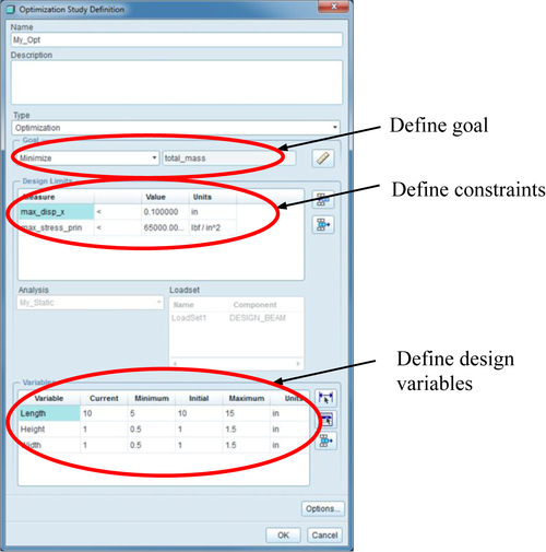
In the Optimization Study Definition dialog box (Figure P5.3) that appears after choosing File > New Optimization Design Study, users may define a design optimization problem by choosing a measure as the objective function. Measures are predefined physical quantities, such as mass, maximum principal stress, and so forth, provided by Mechanica after an FEA run. Mechanica only supports single-objective optimization problems; hence, only one measure can be included in the objective.

Similar to the goal, users may choose measures to define constraints. For the condition, you may select one of the following three options: (1) “>” is greater than the minimum acceptable value, (2) “<” is less than the maximum acceptable value, and (3) “=” is equal to the given value.

Users may choose continuous variables to perform optimization. For each design variable, users need to define its lower and upper limits. Dimensions of the solid model are the most common variables for optimization. In addition, parameters, such as material properties, can also be chosen as design variables. Note that the model, part, or assembly must be fully parameterized to conduct a batch-mode optimization in Pro/ENGINEER, as discussed in Chapter 3. More about design parameterization can be found in Chang (2014).

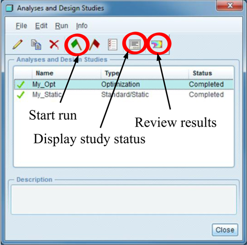
FIGURE P5.2 Analyses and Design Studies dialog box.

FIGURE P5.3 Optimization Study Definition dialog box.

Once an optimization problem is completely defined, users may simply click the Start run

button (see Figure P5.2) to launch optimization. During the run, users may click Display study status button

to see the status of the optimization. At the end of the run, users may choose the Review results

to review the results of the study, such as a history plot of the objective function, as shown in Figure P5.4.

P5.1.2. Tutorial Examples

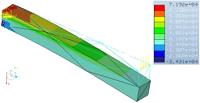
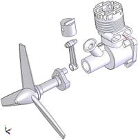
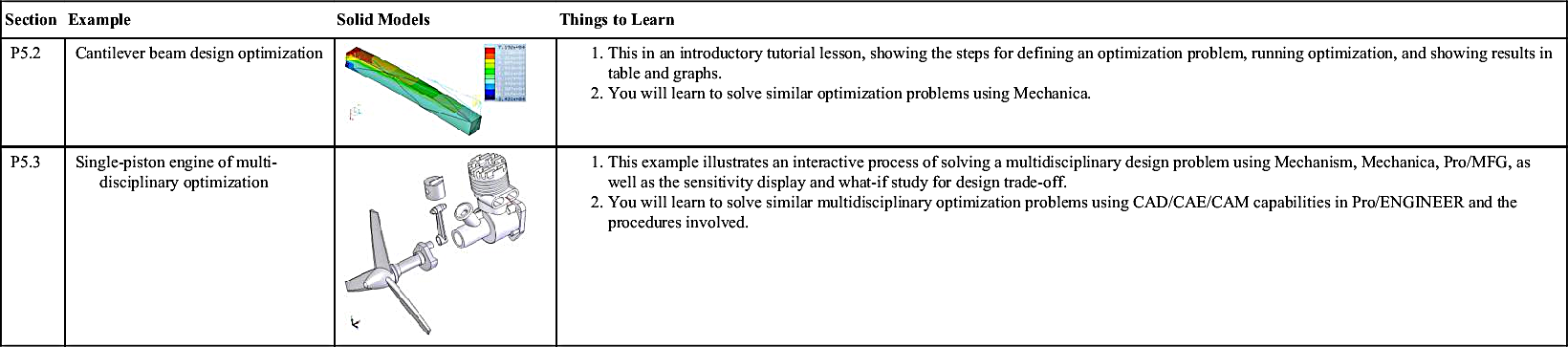
Two examples are included in this tutorial project. The first example, cantilever beam, illustrates the step-by-step details of defining an optimization problem, running the optimization, and showing results in data and graphs. The second example, a single-piston engine, illustrates an interactive design process of solving a multidisciplinary design problem using Mechanism, Mechanica, Pro/MFG, as well as the sensitivity display and what-if study discussed in Chapter 3. Because the detailed steps in using individual software modules have been discussed in Projects P1–P4, we only include the major steps with key information in these examples. Examples and topics to be discussed in each lesson are summarized in Table P5.1.

P5.2. Cantilever Beam

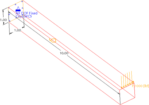
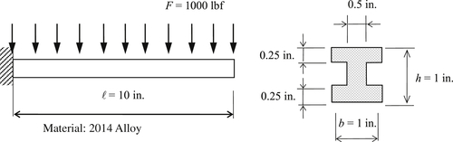
We use the cantilever beam example shown in Chapter 3 to illustrate the steps for carrying out design optimization using Pro/ENGINEER. The beam is again shown in Figure P5.5 for illustration. The beam is made of AL2014. At the current design, the beam length is ℓ = 10 in., and the width w and height h of the crosssectional area are both 1 in. The load is P = 1000 lbf acting vertically at the tip of the beam, as shown in Figure P5.5. Our goal is to optimize the beam design for a minimum mass subject to displacement and stress constraints by varying its length as well as the width and height of the cross-section.

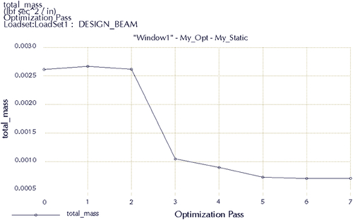
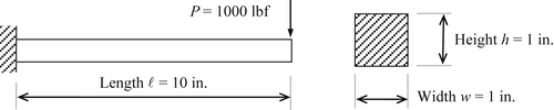
FIGURE P5.4 Objective function history graph.

Table P5.1

Examples Employed in This Project

Section	Example	Solid Models	Things to Learn
P5.2	Cantilever beam design optimization		1. This in an introductory tutorial lesson, showing the steps for defining an optimization problem, running optimization, and showing results in table and graphs. 2. You will learn to solve similar optimization problems using Mechanica.
P5.3	Single-piston engine of multi-disciplinary optimization		1. This example illustrates an interactive process of solving a multidisciplinary design problem using Mechanism, Mechanica, Pro/MFG, as well as the sensitivity display and what-if study for design trade-off. 2. You will learn to solve similar multidisciplinary optimization problems using CAD/CAE/CAM capabilities in Pro/ENGINEER and the procedures involved.

Section

Example

Solid Models

Things to Learn

P5.2

Cantilever beam design optimization

1. This in an introductory tutorial lesson, showing the steps for defining an optimization problem, running optimization, and showing results in table and graphs.

2. You will learn to solve similar optimization problems using Mechanica.

P5.3

Single-piston engine of multi-disciplinary optimization

1. This example illustrates an interactive process of solving a multidisciplinary design problem using Mechanism, Mechanica, Pro/MFG, as well as the sensitivity display and what-if study for design trade-off.

2. You will learn to solve similar multidisciplinary optimization problems using CAD/CAE/CAM capabilities in Pro/ENGINEER and the procedures involved.

P5.2.1. Design Problem Definition

The design problem of the cantilever beam example is formulated mathematically as:

$Minimize : M (w, h, ℓ) = ρ w h ℓ$ $Minimize : M (w, h, ℓ) = ρ w h ℓ$

(P5.2a)

$Subject to : g_{1} (w, h, ℓ) = σ_{mp} (w, h, ℓ) - 65 ksi \leq 0$ $Subject to : g_{1} (w, h, ℓ) = σ_{mp} (w, h, ℓ) - 65 ksi \leq 0$

(P5.2b)

$g_{2} (w, h, ℓ) = δ_{x} (w, h, ℓ) - 0.1 in . \leq 0$ $g_{2} (w, h, ℓ) = δ_{x} (w, h, ℓ) - 0.1 in . \leq 0$

(P5.2c)

$0.5 in . \leq w \leq 1.5 in ., 0.5 in . \leq h \leq 1.5 in ., 5 in . \leq ℓ \leq 15 in .$ $0.5 in . \leq w \leq 1.5 in ., 0.5 in . \leq h \leq 1.5 in ., 5 in . \leq ℓ \leq 15 in .$

(P5.2d)

in which ρ is the mass density, σ_mp is the maximum principal stress, and δ_x is the maximum displacement in the X-direction (vertical).

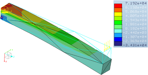
A static design study is created for the beam with boundary and load conditions shown in Figure P5.6. The material chosen is AL2014 from Mechanica material library. The unit system chosen is IPS (in-lbf-s). Also shown in Figure P5.6 are the finite element mesh (with default settings) and the fringe plot of the maximum principal stress (or the measure: max_stress_prin of Mechanica).

In the current design, the maximum principal stress (g₁) is 71.9 ksi, which is greater than the required upper bound 65 ksi. This performance constraint is violated; hence, the design is infeasible.

The second performance constraint, the maximum X-displacement (g₂), is 0.373 in., which is greater than the required upper bound 0.1 in. Again, this performance constraint is violated (the design is infeasible).

We are changing the width, height, and length of the beam to find an optimal solution that is feasible and minimizes the mass of the beam.

P5.2.2. Using Pro/ENGINEER

P5.2.2.1. Open Pro/ENGINEER part

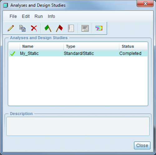
Open the solid model of the cantilever beam downloaded from the book's companion Web site, with the filename: beam.prt.1 in the folder: “Project P5 Examples/Lesson P5.2 Cantilever Beam.” This cantilever example is similar to that of Project P3.2 in Chang (2013a). After opening this file, enter Mechanica and choose Mechanica Analyses/Studies. You should see that there is already a My_Static study created for you. You may want to browse the stress and displacement results of the study. Also, please check the unit system (File > Properties), and take a look at the finite element mesh. Again, the IPS Unit system is employed for this lesson.

FIGURE P5.6 Finite element model and stress fringe plot of the cantilever beam in Mechanica.

P5.2.2.2. Create a new design study

In the Analyses and Design Studies dialog box (Figure P5.7), a My_Static study is listed. From the pull-down menu of the Analyses and Design Studies dialog box, choose:

File > New Optimization Design Study.

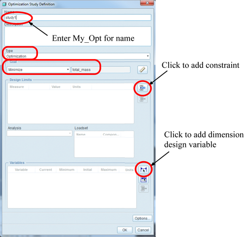
In the Optimization Study Definition dialog box (Figure P5.8), enter or choose the following:

• Enter the name of the design study as My_Opt

• Enter description (optional)

• Choose Optimization for Type (default)

• Select the total_mass as the objective function to be minimized (default).

P5.2.2.3. Add constraints

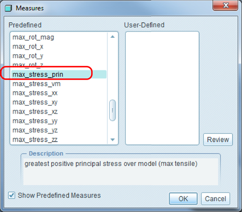
Define the performance constraint function by clicking the button

to the right of the “Design Limits” area in the Optimization Study Definition dialog box (see Figure P5.8). The Measures dialog box appears (see Figure P5.9). In the Measures dialog box, scroll down the Predefined (left) column to choose max_stress_prin, and click OK.

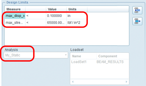
The max_stress_prin measure will be listed under the “Design Limits.” Choose “<” (default), and enter 65,000 as the limit. Make sure the unit is lbf/in.² (psi). Repeat the same steps to choose max_disp_x, choose “<,” and enter 0.1 as the limit for the second constraint, as shown in Figure P5.10. The unit is inches. Note that My_Static was chosen by default and listed under Analysis (see Figure P5.10).

FIGURE P5.7 Analyses and Design Studies dialog box.

P5.2.2.4. Add design variables

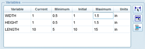
Now, we define design variables. Click the first button

to the right of the “Variables” area in the Optimization Study Definition dialog box (see Figure P5.8), and click the beam in the graphics window (dimensions will appear like those in Figure P5.11). Pick the length dimension; the dimension will be listed under the “Variables” area in the Optimization Study Definition dialog box (see Figure P5.12). Enter LENGTH for name, and 5 and 15 for Minimum and Maximum, respectively.

Repeat the same steps for the height and width dimension variables. Enter HEIGHT and WIDTH for names. Enter 0.5 and 1.5 for Minimum and Maximum, respectively, for both variables.

Note that the Options button at the lower right corner of the Optimization Study Definition dialog box allows users to define design study options, including optimization algorithm, convergence tolerance, and number of iterations. We will use default settings for this problem (convergence tolerance: 1.0% and number of iterations: 20). Now, a design optimization problem is completely defined. Click OK in the Optimization Study Definition dialog box. The My_Opt design study is now listed in the Analyses and Design Studies dialog box. We are ready to run an optimization design study.

FIGURE P5.8 The Optimization Study Definition dialog box.

FIGURE P5.10 Constraint functions defined.

FIGURE P5.11 Pick the length dimension in the graphics window.

FIGURE P5.12 All three dimension variables defined.

P5.2.2.5. Run optimization

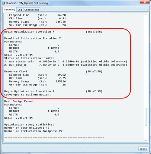
In the Analyses and Design Studies dialog box, choose My_Opt and click the Start run button

. Click No to the Question: Do you want to run interactive diagnostics? The optimization starts. You may click the Display study status button

to monitor the run (see Figure P5.13 for a sample status).

At the end, an optimum is found after seven design iterations (see Figure P5.13), in which width, height, and length become 0.5, 1.08, and 5 in., respectively. Displacement is 0.0766 in. (<0.1 in.) and stress is 64.996 psi (<65 ksi). The total mass is 0.0007056 lbf-s²/in. (or 0.2724 lbm), reduced from 0.002614 lbf-s²/in (or 1.009 lbm) from the initial design.

P5.2.2.6. Review results

Here, we will show optimization history graphs of the objective and constraint functions.

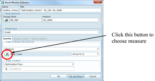
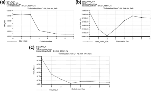
From the Analyses and Design Studies window (Figure P5.7), click the Review result button

(first from the right), the Result Window Definition dialogue box appears (Figure P5.14). Enter Optimization_History for Name, keep all default selections, choose Graph for Display type, and click the Measure button

(see Figure P5.14). In the Measures dialog box, choose total_mass. The total_mass should appear in the Result Window Definition dialogue box. Click OK and Show. The optimization history graph for the objective function appears, like that of Figure P5.15a.

Choose Edit > Results Window to bring the Results Window Definition dialog box back. Repeat the steps to show the graphs for the constraint functions by choosing two respective measures: max_stress_prin and max_disp_x. The graphs should appear like those of Figures P5.15b and c for max_stress_prin and max_disp_x, respectively.

Save your model for future reference.

P5.3. Single-Piston Engine

In this lesson, we provide more details for carrying out the design problem of the single-piston engine (see Figure 1.18) discussed in Chapter 1. Recall in Section 1.5 that a cross-functional team was asked to develop a new model of the engine with a 30% increment in both maximum torque and horsepower at the speed of 1215 rpm. The design of the new engine was carried out at two interrelated levels: the system level and component level. At the system level, due to the increase in power and torque, the bore diameter of the engine case was increased from 1.416 to 1.6 in., the crank length was increased from 0.5833 to 0.72 in., and the connecting road length was increased from 2.25 to 2.49 in., as listed in Table 1.1. Also, the change causes the brake effective pressure P_b to increase from 140 to 180 lbf, causing the peak combustion load to increase from 400 to 600 lbf acting on the top face of the piston. The load magnitude and path applied to the major load-bearing components, such as the connecting rod and crankshaft, are therefore altered. Reaction forces applied to components, such as the connecting rod, increase. The increase in reaction forces raises concerns about the structural integrity of these load-bearing components in the engine. Changes may need to be made to strengthen the design of these components, which may cause an increase in manufacturing time and cost.

FIGURE P5.13 Run Status dialog box. The design converges in seven iterations.

FIGURE P5.14 The Result Window Definition dialogue box.

FIGURE P5.15 Optimization history graphs. (a) Objective function (total_mass). (b) Stress constraint (max_stress_prin). (c) Displacement constraint (max_disp_x).

In Section 1.5, we discussed component-level design using the connecting rod as an example. We included structural analysis for stress, buckling load, and frequency, as well as machining time for the connecting rod. We parameterized the geometry of the connecting rod and selected three dimensions—diameter of the large hole (d₃₂), diameter of the small hole (d₃₁), and thickness (d₇)—as design variables (see Table 1.2). We carried out sensitivity analysis for these structural performance measures and manufacturing time by varying these three design variables. We conducted design trade-off and carried out the what-if study to come up with an improved design for the connecting rod.

In this lesson, we repeat the component-level design of the connecting rod using Mechanism, Mechanica, and Pro/MFG. We start with a motion model of the new design—that is, the changes in bore diameter, crankshaft length, and connecting rod length are made according to the new values shown in Table 1.1. We have prepared the structural model of the connecting rod with simulation results in static, frequency, buckling, and fatigue analyses. Also, a Pro/MFG model was prepared. All are carried out at the new design—that is, the length of the connecting rod is 2.49 in. (increased from 2.25 in.). The objective of this lesson is to demonstrate the steps of conducting an interactive design process to achieve an improved design using the connecting rod example.

We start in Section P5.3.1 by describing the model files needed to carry out this exercise. We briefly describe the simulation results at the current design without showing the detailed steps in creating the models and running the simulations. Readers are encouraged to review tutorial projects P1–P4 for a good standing in solid modeling, motion analysis, structural analysis, and machining simulation, respectively, using Pro/ENGINEER CAD/CAE/CAM tools. With an understanding of the current design of the connecting rod, we move on to conduct sensitivity analysis in Section P5.3.2 and carry out a what-if study in Section P5.3.3. Note that some of the simulation results may not be consistent with those presented in Section 1.5, which were obtained using Mechanism, Mechanica, and Pro/MFG, with slightly different setups.

P5.3.1. Model Files and Current Design

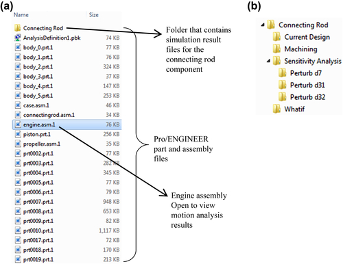
The example files downloaded from the book companion site should contain those shown in Figure P5.16a under the folder named “Project P5 Examples/Lesson P5.3 Single-Piston Engine.” The subfolder named “Connecting Rod” contains another four subfolders: Current Design, Machining, Sensitivity Analysis, and Whatif, as shown in Figure P5.16b. The “Current Design” folder contains simulation result files for the connecting rod at current design, including static, frequency, buckling, and fatigue studies. The “Machining” folder contains Pro/MFG files for machining simulation. Under “Sensitivity Analysis,” there are three subfolders: Perturb d₇, Perturb d₃₁, and Perturb d₃₂. All are empty. We will store perturbed models and simulation results for the respective three design variables for sensitivity analysis using the finite difference method. In the “Whatif” folder, there is a spreadsheet file (Whatif.xlsx) prepared for carrying out a what-if study.

In the following, we briefly go over the models and simulations for motion and structural analyses, as well as machining simulation.

P5.3.1.1. Motion model and simulation

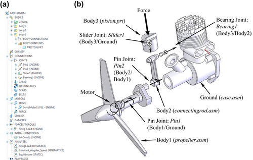
Start Pro/ENGINEER and open “engine.asm.1” under the folder “Lesson P5.3 Single-Piston Engine.” You should see the engine assembly, as shown in Figure P5.17b. There are three subassemblies (case, propeller, and connecting rod) and one part (piston) listed in the model tree (Figure P5.17a).

Enter the Mechanism by choosing from the pull-down menu:

Applications > Mechanism.

FIGURE P5.16 Files and folder under “Lesson P5.3 Single-Piston Engine”: (a) files and subfolder and (b) subfolders included in “Connecting Rod.”

FIGURE P5.17 Engine assembly: (a) model tree, (b) assembly model, and (c) motion model in unexploded view.

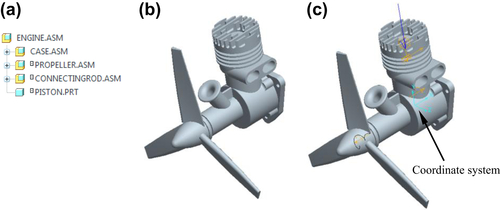
The motion model appears in the graphics area with the motion entity symbols (see Figure P5.17c in an unexploded view), including connections (or joints), force, motor, and so forth. Note the coordinate system chosen is with the Y-axis pointing upward (see Figure P5.17c).

The motion model tree appearing below the model tree lists all motion entities, as shown in Figure P5.18a. There are four rigid bodies (including a Ground body), four joints (Pin1, Pin2, Slider1, and Bearing1), one motor (ServoMotor1) for kinematic analysis, one force (Firing_Load) for dynamic analysis, one initial velocity (InitCond1), and three motion simulations: FiringLoad (DYNAMICS), Constant_Angular_Speed (KINEMATICS), and Equilibrium (STATIC). Note that Equilibrium and Constant_Angular_Speed are created to verify the kinematic characteristics of the motion model. We only use the dynamic simulation (FiringLoad) results for this exercise.

You may want to browse some of the joint definitions to gain a better understanding of the assembly and motion model, especially, “Bearing1” between the connecting rod and piston (Figure P5.18b). This joint is chosen to monitor the reaction force acting on the connecting rod for structural analyses.

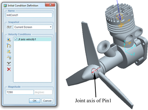
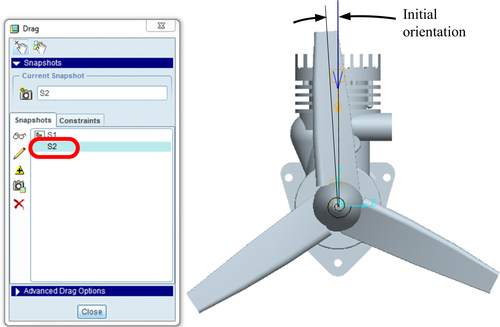
An initial angular velocity is defined and a force is applied to the piston at the beginning of the simulation. The initial velocity of 1215 rpm is defined on the axis of joint Pin1, as shown in Figure P5.19. In Mechanism, one of the approaches in defining the initial position and orientation is using snapshots captured in the Drag Packed Components button

at the top of the graphics window. There are two snapshots captured: S1 and S2. We use S2 as the initial condition to run the dynamic simulation. To impose the condition of snapshot S2, click the Drag component button, and double-click S2 listed in the Drag dialog box shown in Figure P5.20.

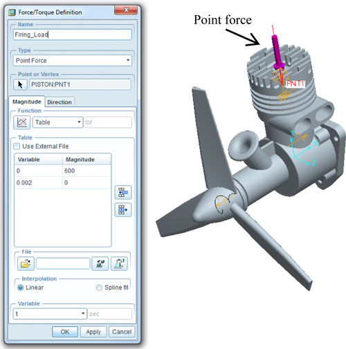
FIGURE P5.18 Engine motion model: (a) motion model tree and (b) motion model in exploded view.

FIGURE P5.19 Initial velocity dialog box.

A force of 600 lbf is applied to the top face of the piston in a short duration of 0.002 s, corresponding to approximately 6.5° of one rotation, as shown in Figure P5.21, to mimic the engine combustion force. Note that the force is applied only once at the beginning of the simulation, which is certainly not realistic. The combustion force cannot be applied to every single combustion cycle accurately due to the limitation of Mechanism capability.

It will be more realistic if the force can be applied when the piston just starts moving downward (negative Y-direction) and can be applied only for a selected short period. To do so, we will have to define measures that monitor the position of the piston for the combustion load to be activated. Unfortunately, such a capability is not available in Mechanism. Therefore, the force is simplified as a step function of 600 lbf along the negative Y-direction and applied for 0.002 s at the beginning of the simulation.

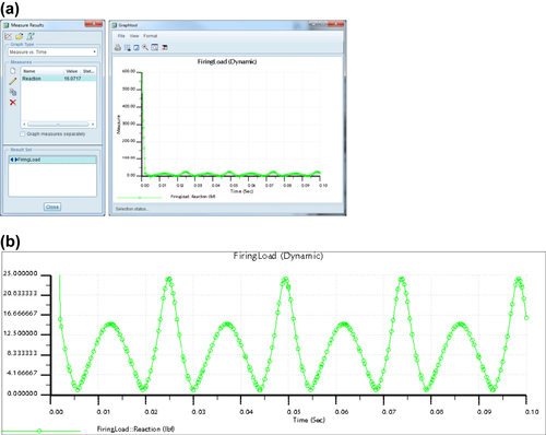
One result plot is created, which shows the reaction force at the upper joint of the connecting rod (Bearing1). To review results in a graph, click the Generate Measure Results of Analyses button

or choose from the pull-down menu:

Analysis > Measures.

The Measure Results dialog box appears (Figure P5.22a). In the Measure Results dialog box, click Reaction (under Measures) and choose FiringLoad (under Result Set), then click the Graph button

at the top left corner to show the graph of reaction force like that of Figure P5.22a.

The reaction force due to inertia can be observed by zooming in the Y-axis, in which the force reaches about 25 lbf, as shown in Figure P5.22b.

For more information regarding using Mechanism, readers are referred to Chang (2011).

FIGURE P5.20 Snapshot S2 defining the initial orientation.

FIGURE P5.21 Force applied at the top face of the piston.

FIGURE P5.22 Reaction force of the Bearing1 joint at top of the connecting rod. (a) Maximum of 600 lbf at the beginning. (b) Zoomed-in view showing small oscillations due to inertia force.

P5.3.1.2. FEA simulations

We now open the connecting rod model (connectingrod.prt) from the subfolder “Connecting Rod/Current Design.” Enter Mechanica by choosing from the pull-down menu:

Applications > Mechanica

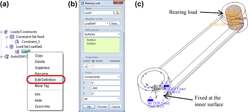
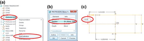
You may review the load and constraint by right-clicking the respective entities in the model tree and choosing Edit Definition. For example, right-click Load1 (see Figure P5.23a) and choose Edit Definition. The Bearing Load dialog box (Figure P5.23b) shows the load data (−600 lbf); in the graphics window, the bearing load is highlighted at the inner surface of the small hole (Figure P5.23c). The inner surface of the large hole is fixed.

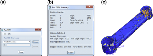
You may check the mesh by choosing from the pull-down menu:

AutoGEM > Create.

FIGURE P5.23 Mechanica model of the connecting rod. (a) Review Load1 by choosing Edit Definition. (b) Bearing Load dialog box. (c) Load and boundary conditions defined.

In the AutoGEM dialog box (Figure P5.24a), click Create. The AutoGEM Summary dialog box (Figure P5.24b) and p-version mesh appear (Figure P5.24c). There are 926 tetrahedron elements in this model. Close the dialog boxes without saving the mesh.

Choose from the pull-down menu:

Analysis > Mechanica Analyses/Studies.

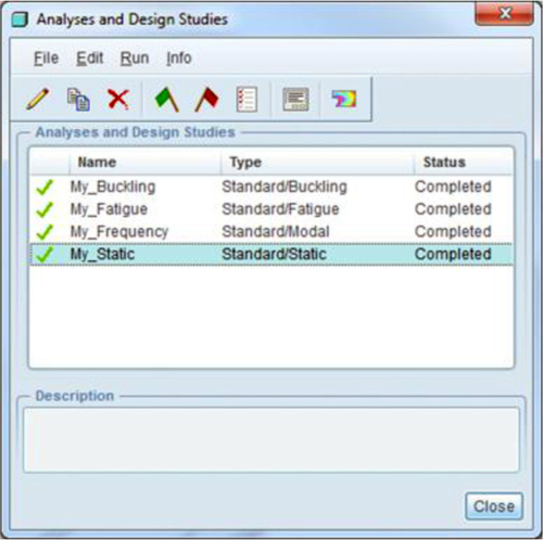
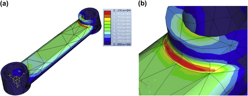
In the Analysis and Study dialog box (Figure P5.25), there are four analyses listed: My_Static, My_Frequency, My_Buckling, and My_Fatigue. These are the four FEA analyses carried out at the connecting rod at current design. You may want to click an analysis and review results. For example, choose My_Static and click the Review results button

(the rightmost) to bring out a fringe plot of von Mises stress, such as that of Figure P5.26a.

The static analysis results show that the maximum von Mises stress occurs in the area of a small fillet between the outer surface of the small cylinder and the exterior surface of the rod, as shown in Figure P5.26b. The maximum stress is 21.91 ksi. The yield strength of the material is about 51 ksi. The safety factor for current design is about 2.33.

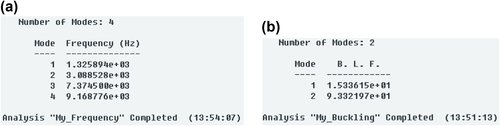
You may choose My_Frequency and click the Display study status button

(second from the right) to bring out the Run Status summary dialog box, in which the first four frequencies are shown (see Figure P5.27a). Similarly, you may see results of My_Buckling analysis (see Figure P5.27b).

As shown in Figure P5.27a, the first (lowest) resonance frequency is 1,326 Hz or 79,560 rpm, which is way higher than the operating frequency in the range of thousands rpm. Also, as shown in Figure P5.27b, the first (lowest) buckling load factor is 15.3, implying that the actual load that causes the connecting rod to buckle is 15.3 × 600 = 9,180 lbf, which is much higher than the firing load.

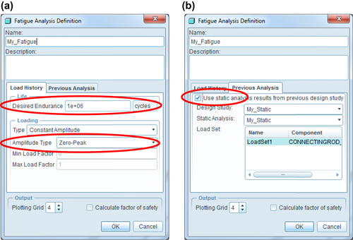
FIGURE P5.24 Finite element mesh of the connecting rod. (a) AutoGEM dialog box. (b) AutoGEM Summary dialog box. (c) The p-version mesh.

FIGURE P5.25 The Analysis and Study dialog box.

For fatigue analysis, we defined the 600-lbf load as a repeated load, where the maximum is 600 lbf and the minimum is 0 (recall a very small inertia force in oscillation). Therefore, we choose the Zero-Peak option, as shown in Figure P5.28a. Also, 1,000,000 cycles is defined for Desired Endurance. Click the Previous Analysis tab to make sure My_Static is chosen for fatigue analysis (Figure P5.28b).

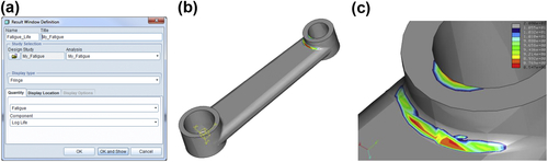
You may display a fringe plot for the fatigue life by following steps similar to those of stress fringe plot (see Figure P5.29a for the Results Window Definition dialog box). The results of fatigue life in the log scale are shown in Figure P5.29b. The lowest and highest lives are 10^8.547 (= 3.52 × 10⁸) to 10²⁰, as seen in the color spectrum of the fringe plot of Figure P5.29c. Essentially, we see infinite fatigue life in the connecting rod. For a more detailed discussion on fatigue analysis using Mechanica, readers are referred to Project P3.4, which is part of Chang (2013a).

FIGURE P5.26 von Mises stress fringe plot. (a) Entire connecting rod model. (b) Zoomed-in view to the high stress concentration area.

FIGURE P5.27 Simulation results: (a) the first four resonance frequencies and (b) the first two buckling load factors.

Close the connecting rod model.

P5.3.1.3. Pro/MFG machining

Manufacturing simulation has also been carried out at the current design. We assume the machining operations start from a green part made by casting, as shown in Figure P5.30a. The machining operations remove materials on the top and bottom faces of the large and small cylinders, and drill two holes, as shown in Figure P5.30b (screen capture made in Vericut).

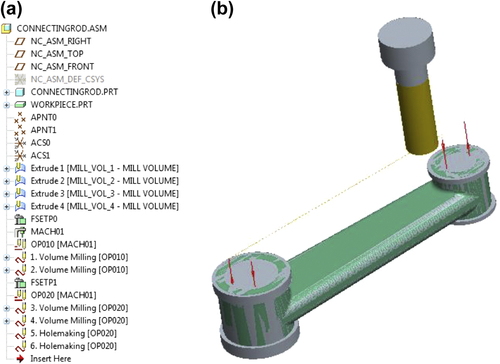
Change the working directory to “Connecting Rod/Machining.” Open the manufacturing (assembly) file “connectingrod.asm.” In the model tree, manufacturing entities are listed as shown in Figure P5.31. In the graphics window, the reference model (connectingrod.prt) and workpiece (workpiece.prt) are assembled properly, as shown in Figure P5.30a.

FIGURE P5.28 Setup for a fatigue analysis: (a) load history definition and (b) using stress of My_Static for the fatigue life calculation.

FIGURE P5.29 Displaying the fatigue life fringe plot. (a) Result Window Definition dialog box. (b) Fatigue life fringe plot. (c) Zoomed-in view.

FIGURE P5.30 Machining simulation. (a) Green part made by casting. (b) Simulation of machining operations (in Vericut).

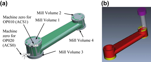
As shown in the model tree (Figure P5.31a), there are two operations: OP010 and OP020, with respective machine zeroes ACS1 and ACS0 (see Figure P5.30a). Two volume milling NC (numerical control) sequences are created under OP010, removing materials defined in Mill Volumes 1 and 2, respectively. Another two volume milling and two hole drilling NC sequences are created for OP020, removing materials of Mill Volume 3 and 4, and drilling the two holes. In practice, jigs and fixtures must be designed and fabricated to hold the green part in support of the machining operations at shop floor. The machine zeroes may need to be adjusted according to the fixture design.

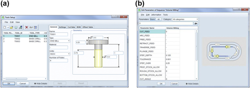
Right-click an NC sequence—for example, 1. Volume Milling—choose Edit Definition, and choose Setup to view how the sequence was defined, including the cutter (see Figure P5.32a) and machining parameters (see Figure P5.32b).

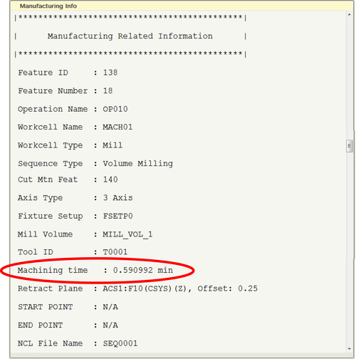
To review the toolpath, you may right-click, for example, OP010 and choose Play Path. Toolpath can be played and shown in the graphics window like that of Figure P5.31b. You may also right-click an NC sequence and choose Info > Feature to find the machining time in the Feature Info window that appears in the graphics window. Scroll down the Feature Info window to find the machining time under the caption of Manufacturing Related Information, as shown in Figure P5.33. Note that this includes only the actual machining time when the cutter is in motion. Setup time, tool change time, and so forth are not included.

The overall machining time is obtained by adding those of individual NC sequences—that is, 0.5910 (1. Volume Milling) + 0.3999 (2. Volume Milling) + 0.6031 (3. Volume Milling) + 0.3904 (4. Volume Milling) + 0.2240 (5. Holemaking) + 0.1941 (6. Holemaking) = 2.403 min.

A more detailed discussion on using Pro/MFG can also be found in Project P4 of Chang (2013b).

P5.3.2. Sensitivity Analysis

The three design variables defined for the connecting rod are the diameter of the larger hole (d₃₂), the diameter of the small hole (d₃₁), and the thickness (d₇). For the current design, the values of the design variables are, respectively, d₃₂ = 0.5 in., d₃₁ = 0.334 in., and d₇ = 0.25 in.

To carry out sensitivity analysis for the gradients of the performance measures, including von Mises stress, lowest resonance frequency, lowest buckling load, fatigue life, mass, and machining time with respect to the three design variables, we use the overall finite difference method discussed in Chapter 3.

FIGURE P5.31 Machining model created in Pro/MFG: (a) model tree and (b) playing toolpath for the machining operation OP010.

FIGURE P5.32 NC sequence setup for volume milling: (a) cutter (Tool Setup) and (b) machining parameters.

FIGURE P5.33 Machining time of a volume milling NC sequence, 1. Volume Milling (OP010).

The approach is very simple. We perturb the individual design variables, one at a time, by 1% of its design variable value. For example, we change the thickness d₇ from 0.25 to 0.2525 in., regenerate the model, and then carry out simulations to find the values of the performance measures at the perturbed design. Thereafter, the sensitivity of a performance ψ(x) can be approximated as:

$\frac{\partial ψ}{\partial x} \approx \frac{ψ (x + Δ x) - ψ (x)}{Δ x}$ $\frac{\partial ψ}{\partial x} \approx \frac{ψ (x + Δ x) - ψ (x)}{Δ x}$

(P5.3)

where ψ(x + Δx) is a performance measure value obtained at the perturbed design from simulation, and Δx is the design perturbation, such as Δd₇ = 0.0025 in.

The detailed steps are described next. We copy the Pro/ENGINEER part file connectingrod.prt from the folder “Connecting Rod/Current Design” and paste it to folders “Connecting Rod/Sensitivity Analysis/Perturb d7,” “Perturb d31,” and “Perturb d32,” respectively.

Then, from Pro/ENGINEER, we open connectingrod.prt from folder “Connecting Rod/Sensitivity Analysis/Perturb d7,” right-click Protrusion id 41, and choose Edit Definition (see Figure P5.34a). In the PROTRUSION: Blend dialog box, double-click Section (see Figure P5.34b). In the sketch appearing in the graphics window, double-click the height dimension and change it to 0.12625 (half of the height, see Figure P5.34c). Click the checkmark

to the right of the graphics window to accept the change. Click OK in the PROTRUSION: Blend dialog box. Choose from the pull-down menu Edit > Regenerate to rebuild the solid model.

FIGURE P5.34 Perturbing design variable (half of d₇) from 0.125 to 0.12625 in. (a) Right-click Protrusion id 41. (b) Choose Section to make the change. (c) Change the height dimension to 0.12625.

Enter Mechanica, choose Analysis > Analysis and Design Studies. Rerun all four studies. Note that My_Static must be carried out before My_Fatigue and My_Buckling because both require the stress results from My_Static study.

Choose My_Static and click the Display study status button

to bring out the Run status window. Find the maximum von Mises stress (max_stress_vm) under Measures. The von Mises stress is now 21.440 ksi. You may create a fringe plot to locate the maximum von Mises stress, which is about the same location as the original design because the perturbation in design variable is small. This value is plugged into Eq. P5.3 to calculate the gradient:

$\frac{\partial ψ}{\partial x} = \frac{\partial σ}{\partial d_{7}} \approx \frac{σ (d_{7} + Δ d_{7}) - σ (d_{7})}{Δ d_{7}} = \frac{21439.8 - 21906.3}{0.0025} = - 1.866 \times 10^{5} psi/in .$ $\frac{\partial ψ}{\partial x} = \frac{\partial σ}{\partial d_{7}} \approx \frac{σ (d_{7} + Δ d_{7}) - σ (d_{7})}{Δ d_{7}} = \frac{21439.8 - 21906.3}{0.0025} = - 1.866 \times 10^{5} psi/in .$

We repeat the same steps to rerun simulations for frequency, buckling, and fatigue. The results are shown in Figure P5.35. The mass of the connecting rod can also be found by choosing Analysis > Model > Mass Properties from the pull-down menu.

Now, we rerun the machining simulation by simply changing the height dimension from 0.125 to 0.12625 in both the reference model and workpiece. Regenerate the models and save them. Then, we open the connectingrod.asm. The reference model and workpiece should both be updated automatically in the assembly. Regenerate the toolpath by replaying the toolpath for all six NC sequences, and then check the machining time.

Note that the machining times are unchanged because the change in the thickness design variable d₇ is not affecting the machining operations, which remove materials at top and bottom faces of the two cylinders and drill two holes for the respective cylinders. Therefore, sensitivity of the machining time with respect to the thickness design variable is zero.

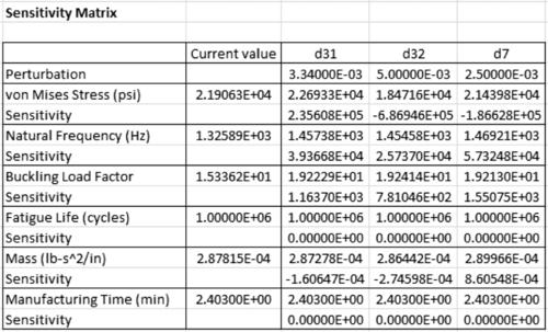
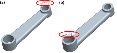
FIGURE P5.35 Sensitivity spreadsheet (in file Whatif.xlsx of Whatif folder).

We repeat the steps discussed above for design variables d₃₁ and d₃₂ by changing them to d₃₂ = 0.505 in. and d₃₁ = 0.33734 in. By simply double-clicking the diameter dimension of the connecting rod in the graphics window, enter the new dimension value (see Figures P5.36a and b) and regenerate the solid model. We carry out simulations and toolpath generations for the two perturbed designs. The sensitivity matrix for the three design variables are calculated as shown in Figure P5.35.

In Figure P5.35, the sensitivity coefficients of the machining time for all three design variables are zero because the design perturbations did not affect the machining operations. Although the hole sizes are changed, we assume the use of drill bits of the same sizes as the holes; therefore, toolpath and machining time are unchanged. Also, the sensitivity coefficients of the fatigue life are all zero because the fatigue life is infinite before and after design perturbations.

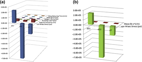
A bar chart of the entire sensitivity coefficient matrix (6 × 3 in this case) can be created using Spreadsheet, as shown in Figure P5.37a. The bar chart provides a global view on the influence of individual design variable to all performance measures and all design variables to a single performance measure. For example, natural frequency increases by increasing any of the three design variables. Among them, d₇ is the most significant and d₃₂ is the least effective. Also, increasing design variable d₇ decreases stress, increases natural frequency, increases buckling load, and so on. Because the sensitivity magnitudes of different measures are different (by an order of magnitude), a common practice is normalizing these gradients by their respective maximum values for a better comparison of the effect of one variable across performance measures.

If we want to reduce stress and not increasing mass by much, we may graph the sensitivity coefficients for these two performance measures only, as can be seen in Figure P5.37b. The bar chart shows that the von Mises stress is reduced by increasing d₃₂ and d₇ and reducing d₃₁. Among them, d₃₂ is the most significant. On the other hand, only a small change in mass is observed.

FIGURE P5.36 Perturb design variables d₃₁ and d₃₂. (a) Change d₃₁ to 0.33734. (b) Change d₃₂ to 0.505.

FIGURE P5.37 Bar chart of the sensitivity matrix. (a) The entire matrix. (b) Selected sensitivity coefficients: stress and mass performance measures.

P5.3.3. What-If Study

We go over a what-if study for the goal of reducing von Mises stress and not increasing the mass of the connecting rod too much. As seen in the bar chart in Figure P5.37b, we perturb all three design variables by using. As discussed in Chapter 3, the steepest decent direction of the stress measure is defined as:

$n = - \frac{{[\frac{\partial σ}{\partial d_{31}} \frac{\partial σ}{\partial d_{32}} \frac{\partial σ}{\partial d_{7}}]}^{T}}{\sqrt{{(\frac{\partial σ}{\partial d_{31}})}^{2} + {(\frac{\partial σ}{\partial d_{32}})}^{2} + {(\frac{\partial σ}{\partial d_{7}})}^{2}}}$ $n = - \frac{{[\frac{\partial σ}{\partial d_{31}} \frac{\partial σ}{\partial d_{32}} \frac{\partial σ}{\partial d_{7}}]}^{T}}{\sqrt{{(\frac{\partial σ}{\partial d_{31}})}^{2} + {(\frac{\partial σ}{\partial d_{32}})}^{2} + {(\frac{\partial σ}{\partial d_{7}})}^{2}}}$

(P5.4)

We then use a small step size, for example α = 0.01, and multiply it with the normalized vector n for design perturbations:

$δ x = α n$ $δ x = α n$

(P5.5)

The design perturbation δx is shown in the cells C29 to E29 of the “Whatif” spreadsheet, as shown in Figure P5.38. The current and predicted performance measure values are listed in Cells F22 to G27, and the percentage changes between them are shown in Cells H22 to H27. The cells indicate that the maximum change is about 48% in Buckling Load Factor, which is large. The stress is reduced by about 35%, with only a 0.045% increase in mass. The design seems to be desirable.

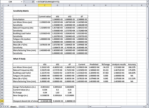
FIGURE P5.38 What-if spreadsheet (in file Whatif.xlsx of Whatif folder).

To carry out simulation of the new design, we first copy the Pro/ENGINEER model of the current design (located in folder: “Connecting Rod/Current Design”) and paste it to folder “Connecting Rod/Whatif.” We then open this model from Pro/ENGINEER and update the solid model by entering the new design variables: d₃₁ = 0.3308578, d₃₂ = 0.5091614, and d₇ = 0.252489. We regenerate the solid model and rerun the simulations. The simulation results are entered to the spreadsheet (Cells I22 to I27); the accuracy of the prediction and analysis results is shown in Cells J22 to J27. The predictions are in general accurate, except for stress. This could be caused by either the insufficient accuracy of the sensitivity or a design perturbation that is not small enough.

In any case, the design is improved with the maximum von Mises stress reduced from 21.91 to 19.11 ksi and a very small increase in mass (0.00028782 to 0.00028793 lb-s²/in.). The process discussed above can be repeated if needed. For the time being, we are satisfied with the design and will stop here.

Question and Exercises

P5.1 Design the following cantilever beam using optimization capability in Mechanica.

Design problem is defined as:

$Minimize : ϕ = ρ b h ℓ (mass)$ $Minimize : ϕ = ρ b h ℓ (mass)$

$Subject to : y_{\max} < 0.1 in .$ $Subject to : y_{\max} < 0.1 in .$

$σ_{vm} < 30 ksi$ $σ_{vm} < 30 ksi$

$0.5 in . < b \leq 1.5 in .$ $0.5 in . < b \leq 1.5 in .$

$0.5 in . < h \leq 3 in .$ $0.5 in . < h \leq 3 in .$

a. Create Pro/ENGINEER and Mechanica models, then carry out optimization. Submit screen captures for the stress and displacement at the initial and optimal designs found by Mechanica. Submit design history graphs for the objective and constraints.

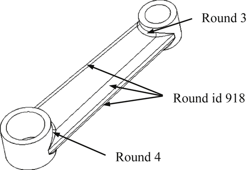
b. Solve the same problem by adjusting the two design variables manually. Is your design better than that of Mechanica? If so, by how much (e.g., mass %)? Submit screen captures for the stress and displacement of the improved design.

P5.2 Carry out sensitivity analysis and at least one what-if study for the connecting rod, following steps similar to that of Section P5.3. In this exercise, we use the same performance measures and three design variables: thickness (d₇, same as that of Section P5.3), and the two groups of fillets shown in the figure below. That is, fillets of radius R 0.04 in. (Round 3 and Round 4) and fillets of radius R 0.09 in. (Round id 918).

Use AL2014 as the material (assuming a yield strength of 25 ksi and endurance limit of 20.5 ksi). The final design must be feasible; that is, the maximum von Mises stress must be less than the yield strength divided by a safety factor of 1.2, fatigue life must be infinite, resonance frequency must be greater than the operating frequency (2000 rpm), and buckling load factor must be greater than the firing load of 600 lbf, with a safety factor of 1.2. Report the following:

a. Simulation results for the current design, including maximum von Mises stress, frequency, buckling load, fatigue life, and mass. Is the current design feasible? If not identify the performance measures that are over the limits (with safety factors considered).

b. Sensitivity matrix, including how you perturbed the three design variables; for example, is 1% perturbation adequate for all three design variables?

c. Report how you came up with a feasible design.

d. Describe how you continue reducing the mass of the connecting rod once you are in the feasible region, if possible.

..................Content has been hidden....................

You can't read the all page of ebook, please click here login for view all page.

Table of Contents for Project P5. Design with Pro/ENGINEER

Create new playlist

Sign In

Sign Up